Flag arrangements and triangulations of products of simplices.

Flag arrangements and 

triangulations of products of simplices. 

Federico Ardila ∗ 

Sara Billey ∗ 

Abstract 

We investigate the line arrangement that results from intersecting 

d complete flags in C n . We give a combinatorial description of the 

matroid T n,d that keeps track of the linear dependence relations among 

these lines. 

We prove that the bases of the matroid T n,3 characterize the triangles 

with holes which can be tiled with unit rhombi. More generally, 

we provide evidence for a conjectural connection between the matroid 

T n,d , the triangulations of the product of simplices ∆ n−1 × ∆ d−1 , and 

the arrangements of d tropical hyperplanes in tropical (n − 1)-space. 

Our work provides a simple and effective criterion to ensure the 

vanishing of many Schubert structure constants in the flag manifold, 

and a new perspective on Billey and Vakil’s method for computing the 

non-vanishing ones. 

1 Introduction. 

Let E 1 •, . . . , E d • be d generically chosen complete flags in C n . We will work 

over the field C of complex numbers, although our results hold over any 

sufficiently large field. Write 

E k • = {{0} = E k 0 ⊂ E k 1 ⊂ · · · ⊂ E k n = C n }, 

where Ei 

k is a vector space of dimension i. Consider the set E n,d of onedimensional 

intersections determined by the flags; that is, all lines of the 

form Ea 1 1 

∩ Ea 2 2 

∩ · · · ∩ Ea d d 

. 

∗ Both authors supported by NSF grant DMS-9983797. 

Date: February 1, 2007 

Keywords: matroids, permutation arrays, Schubert calculus, tropical hyperplane arrangements, 

Littlewood-Richardson coefficients 

1

The initial goal of this paper is to characterize the line arrangements 

C n which arise in this way from d generically chosen complete flags. We 

will then show an unexpected connection between these line arrangements 

and an important and ubiquitous family of subdivisions of polytopes: the 

triangulations of the product of simplices ∆ n−1 ×∆ d−1 . These triangulations 

appear naturally in studying the geometry of the product of all minors of 

a matrix [3], tropical geometry [11], and transportation problems [42]. To 

finish, we will illustrate some of the consequences that the combinatorics of 

these line arrangements have on the Schubert calculus of the flag manifold. 

The results of the paper are roughly divided into four parts as follows. 

First of all, Section 2 is devoted to studying the line arrangement determined 

by the intersections of a generic arrangement of hyperplanes. This will serve 

as a warmup before we investigate generic arrangements of complete flags, 

and the results we obtain will be useful in that investigation. 

The second part consists of Sections 3, 4 and 5, where we will characterize 

the line arrangements that arise as intersections of a “matroid-generic” 

arrangement of d flags in C n . Section 3 is a short discussion of the combinatorial 

setup that we will use to encode these geometric objects. In Section 

4, we propose a combinatorial definition of a matroid T n,d . In Section 5 we 

will show that T n,d is the matroid of the line arrangement of any d flags in 

C n which are generic enough. Finally, we show that these line arrangements 

are completely characterized combinatorially: any line arrangement in C n 

whose matroid is T n,d arises as an intersection of d flags. 

The third part establishes a surprising connection between these line 

arrangements and an important class of subdivisions of polytopes. The 

bases of T n,3 exactly describe the ways of punching n triangular unit holes 

into the equilateral triangle of size n, so that the resulting holey triangle 

can be tiled with unit rhombi. A consequence of this is a very explicit 

geometric representation of T n,3 . We show these results in Section 6. We 

then pursue a higher-dimensional generalization of this result. In Section 7, 

we suggest that the fine mixed subdivisions of the Minkowski sum n∆ d−1 

are an adequate (d − 1)-dimensional generalization of the rhombus tilings 

of holey triangles. We give a completely combinatorial description of these 

subdivisions. Finally, in Section 8, we prove that each fine mixed subdivision 

of the Minkowski sum n∆ d−1 (or equivalently, each triangulation of the 

product of simplices ∆ n−1 ×∆ d−1 ) gives rise to a basis of T n,d . We conjecture 

that every basis of T n,d arises in this way. In fact, it may be true that 

every basis of T n,d arises from a regular subdivision or, equivalently, from 

an arrangement of d tropical hyperplanes in tropical (n − 1)-space. 

2

The fourth and last part of the paper, Section 9, presents some of the 

consequences of our work in the Schubert calculus of the flag manifold. We 

start by recalling Eriksson and Linusson’s permutation arrays, and Billey 

and Vakil’s related method for explicitly intersecting Schubert varieties. In 

Section 9.1 we show how the geometric representation of the matroid T n,3 

of Section 6 gives us a new perspective on Billey and Vakil’s method for 

computing the structure constants c uvw of the cohomology ring of the flag 

variety. Finally, Section 9.2 presents a simple and effective criterion for 

guaranteeing that many Schubert structure constants are equal to zero. 

We conclude with some future directions of research that are suggested 

by this project. 

2 The lines in a generic hyperplane arrangement. 

Before thinking about flags, let us start by studying the slightly easier problem 

of understanding the matroid of lines of a generic arrangement of m 

hyperplanes in C n . We will start by presenting, in Proposition 2.1, a combinatorial 

definition of this matroid H n,m . Theorem 2.2 then shows that this 

is, indeed, the right matroid. As it turns out, this warmup exercise will play 

an important role in Section 5. 

Throughout this section, we will consider a generic central 1 hyperplane 

arrangement, consisting of m hyperplanes H 1 , . . . , H m in C n . For each subset 

A of [m] = {1, 2, . . . , m}, let 

H A = ⋂ a∈A 

H a . 

By genericity, 

dim H A = 

{ n − |A| if |A| ≤ n, 

0 otherwise. 

Therefore, the set L n,m of one-dimensional intersections of the H i s consists 

of the ( m 

n−1) 

lines HA for |A| = n − 1. 

There are several “combinatorial” dependence relations among the lines 

in L n,m , as follows. Each t-dimensional intersection H B (where B is an 

(n − t)-subset of [m]) contains the lines H A with B ⊆ A. Therefore, in 

an independent set H A1 , . . . , H Ak of L n,m , we cannot have t + 1 A i s which 

contain a fixed (n − t)-set B. 

1 A hyperplane arrangement is central if all its hyperplanes go through the origin. 

3

At first sight, it seems intuitively clear that, in a generic hyperplane arrangement, 

these will be the only dependence relations among the lines in 

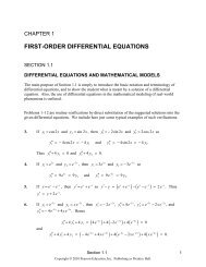
L n,m . This is not as obvious as it may seem: let us illustrate a situation 

in L 4,5 which is surprisingly close to a counterexample to this statement. 

For simplicity, we will draw the three-dimensional projective picture. Each 

hyperplane in C 4 will now look two-dimensional, and the lines in the arrangement 

L 4,5 will look like points. Denote hyperplanes H 1 , . . . , H 5 simply 

by 1, . . . , 5, and an intersection like H 124 simply by 124. 

In Figure 1, we have started by drawing the triangles T and T ′ with vertices 

124, 234, 134 and 125, 235, 135, respectively. The three lines connecting 

the pairs (124, 125), (234, 235) and (134, 135), are the lines 12, 23, and 13, 

respectively. They intersect at the point 123, so that the triangles T and T ′ 

are perspective with respect to this point. 

134 

125 

234 

123 

235 

124 

135 

345 

145 

245 

Figure 1: The Desargues configuration in L 4,5 . 

Now Desargues’ theorem applies, and it predicts an unexpected dependence 

relation. It tells us that the three points of intersection of the corresponding 

sides of T and T ′ are collinear. The lines 14 (which connects 

124 and 134) and 15 (which connects 125 and 135) intersect at the point 

145. Similarly, 24 and 25 intersect at 245, and 34 and 35 intersect at 345. 

Desargues’ theorem says that the points 145, 245, and 345 are collinear. 

In principle, this new dependence relation does not seem to be one of our 

predicted “combinatorial relations”. Somewhat surprisingly, it is: it simply 

states that these three points are on the line 45. 

The previous discussion shows that even five generic hyperplanes in C 4 

give rise to interesting geometric configurations. In this case, we might 

consider ourselves fortunate, because the conclusion of Desargues’ theorem 

was also a consequence of our combinatorial relations. However, it is not 

4

unreasonable to think that larger arrangements L n,m will contain other configurations, 

which have nontrivial dependence relations that we may not 

have predicted. 

Having told our readers what they might need to worry about, we now 

intend to convince them not to worry about it. 

First we show that the combinatorial dependence relations in L n,m are 

consistent, in the sense that they define a matroid. This statement will 

follow as a consequence of Theorem 2.2. We now give a different proof, 

which sheds light on the combinatorial structure of the matroid. 

Proposition 2.1. Let I consist of the collections I of subsets of [m], each 

containing n − 1 elements, such that no t + 1 of the sets in I contain an 

(n − t)-set. In symbols, 

I := 

{ 

I ⊆ 

( ) [m] 

n − 1 

such that for all S ⊆ I, 

∣ ⋂ A ∣ } 

≤ n − |S| . 

A∈S 

Then I is the collection of independent sets of a matroid H n,m . 

Proof. A circuit of that matroid would be a minimal collection C of s subsets 

of [m] of size n − 1, all of which contain one fixed (n − s + 1)-set. It suffices 

to verify the circuit axioms: 

(C1) No proper subset of a circuit is a circuit. 

(C2) If two circuits C 1 and C 2 have an element x in common, then C 1 ∪C 2 −x 

contains a circuit. 

The first axiom is satisfied trivially. Now consider two circuits C 1 and 

C 2 containing a common (n − 1)-set X 1 . Let 

C 1 = {X 1 , . . . , X a , Y 1 , . . . , Y b }, C 2 = {X 1 , . . . , X a , Z 1 , . . . , Z c }, 

where the Y i s and Z i s are all distinct. Write 

X = 

a⋂ 

X i , Y = 

i=1 

b⋂ 

Y i , Z = 

i=1 

c⋂ 

Z i . 

By definition of C 1 and C 2 we have that |X ∩ Y | ≥ n − (a + b) + 1 and 

|X ∩ Z| ≥ n − (a + c) + 1, and their minimality implies that |X| ≤ n − a. 

Therefore 

|X ∩ Y ∩ Z| = |X ∩ Y | + |X ∩ Z| − |(X ∩ Y ) ∪ (X ∩ Z)| 

≥ 

|X ∩ Y | + |X ∩ Z| − |X| 

i=1 

≥ (n − a − b + 1) + (n − a − c + 1) − (n − a) 

= n − a − b − c + 2, 

5

and hence 

|X 2 ∩ · · · ∩ X a ∩ Y 1 ∩ · · · ∩ Y b ∩ Z 1 ∩ · · · ∩ Z c | ≥ n − (a + b + c − 1) + 1. 

It follows that C 1 ∪ C 2 − X 1 contains a circuit, as desired. 

Now we show that this matroid H n,m is the one determined by the lines 

in a generic hyperplane arrangement. 

Theorem 2.2. If a central hyperplane arrangement A = {H 1 , . . . , H m } in 

C n is generic enough, then the matroid of the ( m 

n−1) 

lines HA is isomorphic 

to H n,m . 

Proof. We already observed that the one-dimensional intersections of A satisfy 

all the dependence relations of H n,m . Now we wish to show that, if A 

is generic enough, these are the only relations. 

Any hyperplane arrangement can be constructed as follows. Consider 

the m coordinate hyperplanes in C m , numbered J 1 , . . . , J m . Pick an n- 

dimensional subspace V of C m , and consider the ((n − 1)-dimensional) arrangement 

of hyperplanes H 1 = J 1 ∩ V, . . . , H m = J m ∩ V in V . We will see 

that, if V is generic enough in the sense of Dilworth truncations, then the 

arrangement {H 1 , . . . , H m } is generic enough for the conclusion of Theorem 

2.2 to hold. We now recall this setup. 

Theorem 2.3. (Brylawski, Dilworth, Mason, [7, 8, 29]) Let L be a set of 

lines in C r whose corresponding matroid is M. Let V be a subspace of C r 

of codimension k − 1. For each k-flat F spanned by L, let v F = F ∩ V . 

1. If V is generic enough, then each v F is a line, and the matroid D k (M) 

of the lines v F does not depend on V . 

2. The circuits of D k (M) are the minimal sets {v F1 , . . . , v Fa } such that 

rk M (F 1 ∪· · ·∪F a ) ≤ a+k−2. 2 This matroid is called the k-th Dilworth 

truncation of M. 3 

2 The idea behind this is that, if the span of F 1, . . . , F a has dimension less than a + 

k − 1, then, upon intersection with V (which has codimension k − 1), their span will have 

dimension less than a. 

3 The matroid D k (M) can be defined combinatorially by specifying its circuits in the 

same way, even if M is not representable. In fact, when M is representable, the most subtle 

aspect of our definition of D k (M) is the construction of a sufficiently generic subspace V , 

and hence of a geometric realization of D k (M). This construction was proposed by Mason 

[29] and proved correct by Brylawski [7]. They also showed that, if M is not realizable, 

then D k (M) is not realizable either. 

6

This is precisely the setup that we need. Let L = {1, . . . , m} be the 

coordinate axes of C m , labelled so that coordinate hyperplane J i is normal 

to axis i. These m lines are a realization of the free matroid M m on m 

elements. 

Now consider the (m − n + 1)-th Dilworth truncation D m−n+1 (M m ) 

of M m , obtained by intersecting our configuration with an n-dimensional 

subspace V of C m , which is generic enough for Theorem 2.3 to apply. For 

each (m − n + 1)-subset T of L = {1, . . . , m}, we get an element of the 

matroid of the form 

(⋂ ) 

v T = (span T ) ∩ V = J i ∩ V = ⋂ (J i ∩ V ) = ⋂ H i = H [m]−T , 

i/∈T 

i/∈T 

i/∈T 

where, as before, H i = J i ∩ V is a hyperplane in V . Since ∣ ∣[m] − T ∣ = 

n − 1, this v T is precisely one of the lines in the arrangement L n,m of onedimensional 

intersections of {H 1 , . . . , H m }. In Theorem 2.3, we have a combinatorial 

description for the matroid D m−n+1 (M m ) of the v T s. It remains 

to check that this matches our description of H n,m . 

This verification is straightforward. In D m−n+1 (M m ), the collection 

{v T1 , . . . , v Ta } is a circuit if it is a minimal set such that the following equivalent 

conditions hold: 

rk Mm (T 1 ∪ · · · ∪ T a ) ≤ a + (m − n + 1) − 2, 

|T 1 ∪ · · · ∪ T a | ≤ m − (n − a + 1), 

|([m] − T 1 ) ∩ · · · ∩ ([m] − T a )| ≥ n − a + 1. 

This is equivalent to {[m] − T 1 , . . . , [m] − T a } being a circuit of the matroid 

H n,m , which is precisely what we wanted to show. This completes the proof 

of Theorem 2.2. 

Corollary 2.4. The matroid H n,m is isomorphic to the (m − n + 1)-th 

Dilworth truncation of the free matroid M m . 

Proof. This is an immediate consequence of our proof of Theorem 2.2. 

Comment. Given a hyperplane arrangement A, Manin and Schechtman 

[27] and Bayer and Brandt [5] studied the space U(A) of arrangements of 

hyperplanes which are in the most general position possible, while staying 

parallel to the hyperplanes of A. They showed that this space is itself the 

complement of a central hyperplane arrangement B(A), called the discriminantal 

arrangement of A. 

7

Their construction is closely related to ours, as observed by Falk [14] 

and Bayer and Brandt [5]. Let H and H ∗ be dual hyperplane arrangements 

in the matroid sense. Then the arrangement of lines determined by H is 

linearly isomorphic to the arrangement of lines normal to the discriminantal 

arrangement of H ∗ . In particular, Theorem 2.2 follows from this circle of 

ideas; see [2, 9, 14, 27]. 

3 From lines in a flag arrangement to lattice points 

in a simplex. 

Having understood the matroid of lines in a generic hyperplane arrangement, 

we proceed to study the case of complete flags. In the following three 

sections, we will describe the matroid of lines of a generic arrangement of d 

complete flags in C n . We start, in this section, with a short discussion of the 

combinatorial setup that we will use to encode these geometric objects. We 

then propose, in Section 4, a combinatorial definition of the matroid T n,d . 

Finally, we will show in Section 5 that this is, indeed, the matroid we are 

looking for. 

Let E 1 •, . . . , E d • be d generically chosen complete flags in C n . Write 

E k • = {{0} = E k 0 ⊂ E k 1 ⊂ · · · ⊂ E k n = C n }, 

where Ei k is a vector space of dimension i. 

These d flags determine a line arrangement E n,d in C n as follows. Look 

at all the possible intersections of the subspaces under consideration; they 

are of the form E a1 ,...,a d 

= Ea 1 1 

∩ Ea 2 2 

∩ · · · ∩ Ea d d 

. We are interested in 

the one-dimensional intersections. Since the E• k s were chosen generically, 

E a1 ,...,a d 

has codimension (n − a 1 ) + . . . + (n − a d ) (or n if this sum exceeds 

n). Therefore, the one-dimensional intersections are the lines E a1 ,...,a d 

for 

a 1 + · · · + a d = (d − 1)n + 1. There are ( ) 

n+d−2 

d−1 such lines, corresponding to 

the ways of writing n−1 as a sum of d nonnegative integers n−a 1 , . . . , n−a d . 

Let T n,d be the set of lattice points in the following (d − 1)-dimensional 

simplex in R d : 

{ (x 1 , . . . , x d ) ∈ R d | x 1 + · · · + x d = n − 1 and x i ≥ 0 for all i}. 

The d vertices of this simplex are (n − 1, 0, 0, . . . , 0), (0, n − 1, 0, . . . , 0), . . . , 

(0, 0, . . . , n − 1). For example, T n,3 is simply a triangular array of dots of 

size n; that is, with n dots on each side. We will call T n,d the (d−1)-simplex 

of size n. Each edge contains n dots. 

8

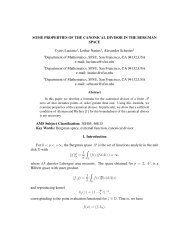
It will be convenient to identify the line E a1 ,...,a d 

(where a 1 + · · · + a d = 

(d − 1)n + 1 and 1 ≤ a i ≤ n) with the vector (n − a 1 , . . . , n − a d ) of codimensions. 

This clearly gives us a one-to-one correspondence between the set 

T n,d and the lines in our line arrangement E n,d . 

E 300 

324 

144 

234 

333 342 

414 

441 

F 

423 

243 

210 201 

G 

120 111 102 

030 021 012 003 

432 

Figure 2: The lines determined by three flags in C 4 , and the array T 4,3 . 

We illustrate this correspondence for d = 3 and n = 4 in Figure 2. This 

picture is easier to visualize in real projective 3-space. Now each one of the 

flags E • , F • , and G • is represented by a point in a line in a plane. The lines 

in our line arrangement are now the 10 intersection points we see in the 

picture. 

We are interested in the dependence relations among the lines in the 

line arrangement E n,d . As in the case of hyperplane arrangements, there 

are several combinatorial relations which arise as follows. Consider a k- 

dimensional subspace E b1 ,...,b d 

with b 1 + · · · + b d = (d − 1)n + k. Every line 

of the form E a1 ,...,a d 

with a i ≤ b i is in this subspace, so no k + 1 of them 

can be independent. The corresponding points (n − a 1 , . . . , n − a d ) are the 

lattice points inside a parallel translate of T k,d , the simplex of size k, in T n,d . 

In other words, in a set of independent lines of our arrangement, we cannot 

have more than k lines whose corresponding dots are in a simplex of size k 

in T n,d . 

For example, no four of the lines E 144 , E 234 , E 243 , E 324 , E 333 , and E 342 

are independent, because they are in the 3-dimensional hyperplane E 344 . 

The dots corresponding to these six lines form the upper T 3,3 found in our 

T 4,3 drawn in Figure 2. 

In principle, there could be other hidden dependence relations among 

the lines in E n,d . The goal of the next two sections is to show that this is 

9

not the case. In fact, these combinatorial relations are the only dependence 

relations of the line arrangement associated to d generically chosen flags in 

C n . 

We will proceed as in the case of hyperplane arrangements. We will 

start by showing, in Section 4, that the combinatorial relations do give rise 

to a matroid T n,d . In Section 5, we will then show that this is, indeed, the 

matroid we are looking for. 

4 A matroid on the lattice points in a regular 

simplex. 

The combinatorial dependence relations defined in Section 3 do in fact determine 

a matroid. This will follow as a consequence of Theorem 5.1. As we 

did in Section 2 for hyperplanes, we will now give an alternative combinatorial 

proof of this statement, which is helpful in understanding the structure 

of the matroid we are interested in. 

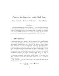
Theorem 4.1. Let I n,d be the collection of subsets I of T n,d such that every 

parallel translate of T k,d contains at most k points of I, for every k ≤ n. 

Then I n,d is the collection of independent sets of a matroid T n,d on the 

ground set T n,d . 

We will call a parallel translate of T k,d a simplex of size k. As an example, 

T n,3 is a triangular array of dots of size n. The collection I n,3 consists of 

those subsets I of the array T n,3 such that no triangle of size k contains 

more than k points of I. Figure 3 shows the array T 4,3 , and a set in I 4,3 . 

Figure 3: The array T 4,3 and a set in I 4,3 . 

Proof of Theorem 4.1. We need to verify the three axioms for the collection 

of independent sets of a matroid: 

(I1) The empty set is in I n,d . 

10

(I2) If I is in I n,d and I ′ ⊆ I, then I ′ is also in I n,d . 

(I3) If I and J are in I n,d and |I| < |J|, then there is an element e in J − I 

such that I ∪ e is in I n,d . 

The first two axioms are satisfied trivially; let us focus on the third one. 

Proceed by contradiction. Let J − I = {e 1 , . . . , e m }. We know that every 

simplex of size a contains at most a points of I. When we try to add e h to 

I while preserving this condition, only one thing can stop us: a simplex T h 

of size t h which already contains t h points of I, and also contains e h . 

Say that a simplex of size t is I-saturated if it contains exactly t points of 

I. We have found I-saturated simplices T 1 , . . . , T m which contain e 1 , . . . , e m , 

respectively. 

Now we use the following lemma, which we will prove in a moment. 

Lemma 4.2. Let T and T ′ be two I-saturated simplices, and let T ∨ T ′ be 

the smallest simplex containing both of them. Suppose that T and T ′ are 

either overlapping or neighboring; that is, either 

1. T ∩ T ′ ≠ ∅, or 

2. T ∩ T ′ = ∅ and size(T ∨ T ′ ) = size(T ) + size(T ′ ). 

Then the simplices T ∩ T ′ and T ∨ T ′ are also I-saturated. 

If two of our I-saturated simplices T g and T h are different and have a 

non-empty intersection, we can replace them both by T g ∨ T h . By Lemma 

4.2, this is also an I-saturated simplex, and it still contains e g and e h . We 

can continue in this way, until we obtain I-saturated simplices T ′ 1 , . . . , T ′ m 

containing e 1 , . . . , e m which are pairwise disjoint (though possibly repeated). 

Let U 1 , . . . , U l be this collection of I-saturated simplices, now listed without 

repetitions. Let U r have size s r , and say it contains i r elements of I − J, 

j r elements of J − I, and h r elements of I ∩ J. 

We know that U r is I-saturated, so s r = i r + h r . We also know that J is 

in I n,d , so s r ≥ j r + h r . Therefore, i r ≥ j r for each r. 

Now, the U r s are pairwise disjoint, so ∑ i r ≤ |I − J| and ∑ j r ≤ |J − I|. 

But in fact, we know that every element of J −I is in some U r , so we actually 

have the equality ∑ j r = |J − I|. Therefore we have 

|J − I| = ∑ j r ≤ ∑ i r ≤ |I − J|. 

This contradicts our assumption that |I| < |J|, and Theorem 4.1 follows. 

11

Proof of Lemma 4.2. First we show that size(T ∩ T ′ ) + size(T ∨ T ′ ) = 

size(T ) + size(T ′ ). This is trivial in the second case of the lemma, so we 

assume that T ∩ T ′ ≠ ∅. 

Each simplex is a parallel translate of some T k,d ; its vertices are given 

by (a 1 + k − 1, a 2 , . . . , a d ), . . . , (a 1 , a 2 , . . . , a d + k − 1) for some a 1 , . . . , a d 

such that ∑ a i = n − k. We denote this simplex by T a1 ,...,a d 

; its size is 

k = n − ∑ a i provided ∑ a i ≤ n. It consists of the points (x 1 , . . . , x d ) with 

x i ≥ a i for each i, and ∑ x i = n − 1. Therefore, T a1 ,...,a d 

⊆ T A1 ,...,A d 

if and 

only if a i ≥ A i for each i. 

It follows that if T = T a1 ,...,a d 

and T ′ = T a ′ 

1 ,...,a ′ are two overlapping 

d 

simplices, then we have: 

T ∩ T ′ = T max(a1 ,a ′ 1 ),...,max(a d,a ′ d ) 

T ∨ T ′ = T min(a1 ,a ′ 1 ),...,min(a d,a ′ d ) . 

So size(T ∩ T ′ ) + size(T ∨ T ′ ) = (n − ∑ max(a i , a ′ i )) + (n − ∑ min(a i , a ′ i )) 

and size(T ) + size(T ′ ) = (n − ∑ a i ) + (n − ∑ a ′ i ). These are equal since 

max(a, a ′ ) + min(a, a ′ ) = a + a ′ for any a, a ′ ∈ R. 

We know that T and T ′ are I-saturated, hence they contain size(T ) and 

size(T ′ ) points of I, respectively. Assume that T ∩T ′ and T ∨T ′ contain x and 

y points of I. Then since we shown that size(T ∩T ′ )+size(T ∨T ′ ) = size(T )+ 

size(T ′ ), we have that x+y ≥ size(T )+size(T ′ ) = size(T ∩T ′ )+size(T ∨T ′ ). 

But I is in I n,d , so x ≤ size(T ∩ T ′ ) and y ≤ size(T ∨ T ′ ). This can only 

happen if equality holds, and T ∩ T ′ and T ∨ T ′ are I-saturated. 

5 This is the right matroid. 

We now show that the matroid T n,d of Section 4 is, indeed, the matroid that 

arises from intersecting d flags in C n which are generic enough. 

Theorem 5.1. If d complete flags E•, 1 . . . , E• d in C n are generic enough, 

then the matroid of the ( ) 

n+d−2 

d−1 lines Ea1 ,...,a d 

is isomorphic to T n,d . 

Proof. As mentioned in Section 3, the one-dimensional intersections of the 

E•s i satisfy the following combinatorial relations: each k dimensional subspace 

E b1 ,...,b d 

with b 1 + · · · + b d = (d − 1)n + k, contains the lines E a1 ,...,a d 

with a i ≤ b i ; therefore, it is impossible for k + 1 of these lines to be independent. 

The subspace E b1 ,...,b d 

corresponds to the simplex of dots which is 

labelled T n−b1 ,...,n−b d 

, and has size n − ∑ (n − b i ) = k. The lines E a1 ,...,a d 

with a i ≤ b i correspond precisely with the dots in this copy of T k,d . So these 

“combinatorial relations” are precisely the dependence relations of T n,d . 

12

Now we need to show that, if the flags are generic enough, these are the 

only linear relations among these lines. It is enough to construct one set of 

flags which satisfies no other relations. 

Consider a set H of d(n − 1) hyperplanes Hj 

i in Cn (for 1 ≤ i ≤ d 

and 1 ≤ j ≤ n − 1) which are generic in the sense of Theorem 2.2, so the 

only dependence relations among their one-dimensional intersections are the 

combinatorial ones. Now, for i = 1, . . . , d, define the flag E• i by: 

E i n−1 = H i n−1 

E i n−2 = H i n−1 ∩ H i n−2 

. 

E i 1 = H i n−1 ∩ H i n−2 ∩ · · · ∩ H i 1, 

We will show that these d flags are generic enough; in other words, the 

matroid of their one-dimensional intersections is T n,d . 

Let us assume that a set S of one-dimensional intersections of the E•s 

i 

is dependent. Since each line in S is a one-dimensional intersection of the 

hyperplanes Hj i , we can apply Theorem 2.2. It tells us that for some t we 

can find t + 1 lines in S and a set T of n − t hyperplanes Hj i which contain 

all of them. 

Our t + 1 lines are of the form 

E a1 ,...,a d 

= Ea 1 1 

∩ · · · ∩ Ea d d 

= (Hn−1 1 ∩ · · · ∩ Ha 1 1 

) ∩ · · · ∩ (Hn−1 d ∩ · · · ∩ Ha d d 

). 

Therefore, if a hyperplane Hj i contains them, so does Hi k 

for any k > j. Let 

us add all such hyperplanes to our set T , to obtain the set 

U = {H 1 n−1, . . . , H 1 b 1 

, . . . , H d n−1, . . . , H d b d 

}, 

where b i is the smallest j for which H i j is in T . The set U contains ∑ (n−b i ) 

hyperplanes, so ∑ (n − b i ) ≥ n − t. 

Each one of our t + 1 lines is contained in each of the hyperplanes in U, 

and therefore in their intersection 

⋂ 

H i j ∈U H i j = E b1 ,...,b d 

, 

which has dimension n − ∑ (n − b i ) ≤ t. 

So, actually, the dependence of the set S is a consequence of one of 

the combinatorial dependence relations present in T n,d . The desired result 

follows. 

13

With Theorem 5.1 in mind, we will say that the complete flags E•, 1 . . . , E• 

d 

in C n are matroid-generic if the matroid of the ( ) 

n+d−2 

d−1 lines Ea1 ,...,a d 

is 

isomorphic to T n,d . 

We conclude this section by showing that the one-dimensional intersections 

of matroid-generic flag arrangements are completely characterized by 

their combinatorial properties. 

Proposition 5.2. If a line arrangement L in C n has matroid T n,d , then 

it can be realized as the arrangement of one-dimensional intersections of d 

complete flags in C n . 

Proof. To make the notation clearer, let us give the proof for d = 3, which 

generalizes trivially to larger values of d. Denote the lines in L by L rst for 

r + s + t = 2n + 1. Consider the three flags E • , F • and G • given by 

E i = span{L rst | r ≤ i} 

F i = span{L rst | s ≤ i} 

G i = span{L rst | t ≤ i} 

for 0 ≤ i ≤ n. Compare this with Figure 2 in the case n = 4. The subspace 

E i , for example, is the span of the lines corresponding to the first i rows of 

the triangle. 

Since L is a representation of the matroid T n,3 , the dimensions of E i , F i , 

and G i are equal to i, which is the rank of the corresponding sets (copies of 

T i,3 ) in T n,3 . 

We now claim that the line arrangement corresponding to E • , F • and 

G • is precisely L. This amounts to showing that E i ∩ F j ∩ G k = L ijk for 

i + j + k = 2n + 1. We know that L ijk is in E i , F j , and G k by definition, so 

we simply need to show that dim(E i ∩ F j ∩ G k ) = 1. 

Assume dim(E i ∩ F j ∩ G k ) ≥ 2. Consider the sequence of subspaces: 

E i ∩ F j ∩ G k ⊆ E i+1 ∩ F j ∩ G k ⊆ · · · ⊆ E n ∩ F j ∩ G k ⊆ 

⊆ E n ∩ F j+1 ∩ G k ⊆ · · · ⊆ E n ∩ F n ∩ G k ⊆ 

⊆ E n ∩ F n ∩ G k+1 ⊆ · · · ⊆ E n ∩ F n ∩ G n . 

There are 1 + (n − i) + (n − j) + (n − k) = n subspaces on this list; the 

first one has dimension at least 2, and the last one has dimension n. By the 

pigeonhole principle, two consecutive subspaces on this list must have the 

same dimension. Since one is contained in the other, these two subspaces 

must actually be equal. So assume that E a−1 ∩ F b ∩ G c = E a ∩ F b ∩ G c ; a 

similar argument will work in the other cases. 

Now, we have a + b + c > i + j + k = 2n + 1, so we can find positive 

integers β ≤ b and γ ≤ c such that a + β + γ = 2n + 1. Then L aβγ is a line 

14

which, by definition, is in E a , F b and G c . It follows that 

L aβγ ∈ E a ∩ F b ∩ G c = E a−1 ∩ F b ∩ G c ⊆ E a−1 . 

This implies that L aβγ is dependent on {L rst | r ≤ a−1}, which is impossible 

since L represents the matroid T n,3 . We have reached a contradiction, which 

implies that dim(E i ∩ F j ∩ G k ) = 1 and therefore E i ∩ F j ∩ G k = L ijk . 

It follows that L is the line arrangement determined by flags E • , F • and 

G • , as we wished to show. 

6 Rhombus tilings of holey triangles and the matroid 

T n,3 . 

Let us change the subject for a moment. 

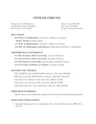
Figure 4: T (4) and the three rhombus tiles. 

Let T (n) be an equilateral triangle with side length n. Suppose we 

wanted to tile T (n) using unit rhombi with angles equal to 60 ◦ and 120 ◦ . 

It is easy to see that this task is impossible, for the following reason. Cut 

T (n) into n 2 unit equilateral triangles, as illustrated in Figure 4; n(n + 1)/2 

of these triangles point upward, and n(n − 1)/2 of them point downward. 

Since a rhombus always covers one upward and one downward triangle, we 

cannot use them to tile T (n). 

Suppose then that we make n holes in the triangle T (n) by cutting out 

n of the upward triangles. Now we have an equal number of upward and 

downward triangles, and it may or may not be possible to tile the remaining 

shape with rhombi. Figure 5 shows a tiling of one such holey triangle. 

The main question we address in this section is the following: 

Question 6.1. Given n holes in T (n), is there a simple criterion to determine 

whether there exists a rhombus tiling of the holey triangle that remains? 

15

Figure 5: A tiling of a holey T (4). 

A rhombus tiling is equivalent to a perfect matching between the upward 

triangles and the downward triangles. Hall’s theorem then gives us an answer 

to Question 6.1: It is necessary and sufficient that any k downward triangles 

have a total of at least k upward triangles to match to. 

However, the geometry of T (n) allows us to give a simpler criterion. 

Furthermore, this criterion reveals an unexpected connection between these 

rhombus tilings and the line arrangement determined by 3 generically chosen 

flags in C n . Notice that the upward triangles in T (n) can be identified with 

the dots of T n,3 . 

Theorem 6.2. Let S be a set of n holes in T (n). The triangle T (n) with 

holes at S can be tiled with rhombi if and only if the locations of the holes 

constitute a basis for the matroid T n,3 ; i.e., if and only if every T (k) in T (n) 

contains at most k holes of S, for all k ≤ n. 

Proof. First suppose that we have a tiling of the holey triangle, and consider 

any triangle T (k) in T (n). Consider all the tiles which contain one or two 

triangles of that T (k), and let R be the holey region that these tiles cover. 

Since all the boundary triangles of T (k) face up, the region R is just T (k) 

with some downward triangles glued to its boundary. 

If T (k) had more than k holes, it would have fewer than k(k − 1)/2 

upward triangles, and so would R. However, R has at least the k(k − 1)/2 

downward triangles of T (k). That makes it impossible to tile the region R, 

which contradicts its definition. This proves the forward direction. 

Now let S be a set of n holes in T (n) such that every T (k) contains at 

most k holes. Equivalently, think of S as a basis of the matroid T n,3 . We 

construct a tiling of the resulting holey triangle by induction on n. The case 

n = 1 is trivial, so assume n ≥ 2. 

Within that induction, we induct on the number of holes of S in the 

bottom row of T (n). Since the T (n − 1) of the top n − 1 rows contains at 

most n − 1 holes, there is at least one hole in the bottom row. 

16

If there is exactly one hole in the bottom row, then the tiling of the 

bottom row is forced upon us, and the top T (n−1) can be tiled by induction. 

Now assume that there are at least two holes in the bottom row; call the two 

leftmost holes x and y in that order. Consider the upward triangles in the 

second to last row which are between x and y; label them a 1 , . . . , a t . This 

is illustrated in an example in the top left panel of Figure 6. Here a 1 , a 2 , a 3 

and a 4 are shaded lightly, and a 1 is also a hole. 

Figure 6: Sliding the hole from a i to x. 

We claim that we can exchange the hole x for one of the holes a i , so that 

the set of holes (S − x) ∪ a i is also a basis of T n,3 . Notice that this a i cannot 

be in S. Assume that no such a i exists. Then each a i must be in a triangle 

T i which is (S − x)-saturated. 4 If a i is in S, then T i = a i . The triangle y 

is also trivially (S − x)-saturated. We can then use Lemma 4.2 successively 

to obtain an (S − x)-saturated triangle containing a 1 , . . . , a t , and y. But 

that triangle will also contain x, so it will contain more holes of S than it is 

allowed. 

So let a i be such that S − x ∪ a i is a basis of T n,3 . For instance, in the 

first step of Figure 6, x is exchanged for a 3 . Notice that S − x ∪ a i contains 

fewer holes in the bottom row than S does. By the induction hypothesis, 

we can tile the T (n) with holes at S − x ∪ a i , as shown in the second step of 

Figure 6. The bottom row of this tiling is frozen from left to right until it 

reaches y. Therefore, we can slide the hole from a i back to x in the obvious 

way, by reversing the tiles in the bottom row between x and a i . This is 

illustrated in the last step of Figure 6. We are left with a tiling with holes 

at S, as desired. 

4 As in Section 4, if A is a set of holes, we say that an upward triangle of size k is 

A-saturated if it contains k holes of A. 

17

Theorem 6.2 allows us to say more about the structure of the matroid 

T n,3 . We first remind the reader of the definition of two important families 

of matroids, called transversal and cotransversal matroids. For more 

information, we refer the reader to [1, 32]. 

Let S be a finite set, and let A 1 , . . . , A r be subsets of S. A transversal of 

(A 1 , . . . , A r ), also known as a system of distinct representatives, is a subset 

{e 1 , . . . , e r } of S such that e i is in A i for each i, and the e i s are distinct. The 

transversals of (A 1 , . . . , A r ) are the bases of a matroid on S. Such a matroid 

is called a transversal matroid, and (A 1 , . . . , A r ) is called a presentation of 

the matroid. 

Let G be a directed graph with vertex set V , and let A = {v 1 , . . . , v r } 

be a subset of V . We say that an r-subset B of V can be linked to A if 

there exist r vertex-disjoint directed paths whose initial vertex is in B and 

whose final vertex is in A. We will call these r paths a routing from B to 

A. The collection of r-subsets which can be linked to A are the bases of a 

matroid denoted L(G, A). Such a matroid is called a cotransversal matroid 

or a strict gammoid. It is a nontrivial fact that these matroids are precisely 

the duals of the transversal matroids [1, 32]. 

Theorem 6.3. The matroid T n,3 is cotransversal. 

First proof. We prove that Tn,3 ∗ is transversal. We can think of the ground 

set of T n,3 as the set of upward triangles in T (n). By Theorem 6.2, a basis 

of T n,3 is a set of n holes for which the resulting holey triangle can be tiled; 

its complement is the set of ( n 

2) 

upward triangles which share a tile with one 

of the ( n 

2) 

downward triangles. 

Number the downward triangles 1, 2, . . . , N = ( n 

2) 

. Then a tiling of the 

complement of a basis of T n,3 is nothing but a transversal of (A 1 , . . . , A N ), 

where A i is the set of three upward triangles which are adjacent to downward 

triangle i. This completes the proof. 

Second proof. We prove that T n,3 is cotransversal. Let G n be the directed 

graph whose set of vertices is the triangular array T n,3 , where each dot not 

on the bottom row is connected to the two dots directly below it. Label the 

dots on the bottom row 1, 2, . . . , n. Figure 7 shows G 4 ; all the edges of the 

graph point down. 

We now recall a trick, commonly used in the tilings literature and attributed 

to Dana Randall, to convert tilings into routings; see for example 

[26]. In our particular situation, it allows us to view rhombus tilings of the 

holey triangle T (n) as routings in G n . The trick works as follows: A copy of 

18

a 

b 

c 

d 

e 

f 

g 

h 

i j k l 

1 

2 3 4 

Figure 7: The graph G 4 . 

the graph G n can be drawn whose vertices are the midpoints of the possible 

horizontal edges of a tiling. Given a tiling of a holey T (n), join two vertices 

of G n if they are on opposite edges of the same tile; this gives the desired 

routing of G n . This correspondence is best understood in an example; see 

Figure 8. 

1 2 3 4 

Figure 8: A tiling of a holey T (4) and the corresponding routing of G 4 . 

Given such a routing, one can easily recover the tiling that gave rise to 

it: simply place one rhombus over each edge in the routing, and one vertical 

rhombus over each isolated vertex. It is easy to check that this is a bijection 

between the rhombus tilings of the holey triangles of size n, and the routings 

in the graph G n which start anywhere and end at vertices 1, 2, . . . , n. 

Notice also that, in this bijection, the holes of the holey triangle correspond 

to the starting points of the n paths in the routing. From Theorem 

6.2, it follows that T n,3 is the cotransversal matroid L(G n , [n]). 

19

Theorem 6.4. Assign sufficiently generic weights to the edges of G n . 5 For 

each dot D in the triangular array T n,3 and each 1 ≤ i ≤ n, let v D,i be the 

sum of the weights of all paths 6 from dot D to dot i on the bottom row. 

Then the path vectors v D = (v D,1 , . . . , v D,n ) are a geometric representation 

of the matroid T n,3 . 

For example, the top dot of T 4,3 in Figure 7 would be assigned the 

path vector (acg, ach + adi + bei, adj + bej + bfk, bfl). Similarly, focusing 

our attention on the top three rows, the representation we obtain for the 

matroid T 3,3 is given by the columns of the following matrix: 

⎛ 

⎝ 

1 0 0 c 0 ac 

0 1 0 d e ad + be 

0 0 1 0 f bf 

Proof of Theorem 6.4. By the Lindström-Gessel-Viennot lemma [17, 20, 25, 

30], the determinant of the matrix with columns v D1 , . . . , v Dn is equal to 

the signed sum of the routings from {D 1 , . . . , D n } to {1, . . . , n}. The sign 

of a routing is the sign of the permutation of S n which matches the starting 

points and the ending points of the n paths. For sufficiently generic weights, 

this signed sum can only equal zero if it is empty. 

Therefore, v D1 , . . . , v Dn are independent if and only if there exists a 

routing from {D 1 , . . . , D n } to {1, . . . , n}. This is equivalent to {D 1 , . . . , D n } 

being a basis of L(G n , [n]). 

It is worth pointing out that Lindström’s original motivation for the 

discovery of the Lindström-Gessel-Viennot lemma was to explain Mason’s 

construction of a geometric representation of an arbitrary cotransversal matroid 

[25, 29]. Theorem 6.4 and its proof are special cases of their more 

general argument; we have included them for completeness. 

The very simple and explicit representation of T n,3 of Theorem 6.4 will 

be shown in Section 9 to have an unexpected consequence in the Schubert 

calculus: it provides us with a reasonably efficient method for computing 

Schubert structure constants in the flag manifold. 

5 We will see that it is enough to choose weights in a certain Zariski open set. 

6 The weight of a path is defined to be the product of the weights of its edges. 

⎞ 

⎠ 

20

7 Fine mixed subdivisions of n∆ d−1 and triangulations 

of ∆ n−1 × ∆ d−1 . 

The surprising relationship between the geometry of three flags in C n and the 

rhombus tilings of holey triangles is useful to us in two ways: it explains the 

structure of the matroid T n,3 , and it clarifies the conditions for a rhombus 

tiling of such a region to exist. We now investigate a similar connection 

between the geometry of d flags in C n , and certain (d − 1)-dimensional 

analogs of these tilings, known as fine mixed subdivisions of n∆ d−1 . 

The fine mixed subdivisions of n∆ d−1 are in one-to-one correspondence 

with the triangulations of the polytope ∆ n−1 × ∆ d−1 . The triangulations of 

a product of two simplices are fundamental objects, which have been studied 

from many different points of view. They are of independent interest [3, 4, 

16], and have been used as a building block for finding efficient triangulations 

of high dimensional cubes [18, 31] and disconnected flip-graphs [40, 41]. 

They also arise very naturally in connection with tropical geometry [11], 

transportation problems, and Segre embeddings [42]. In the following two 

sections, we provide evidence that triangulations of ∆ n−1 × ∆ d−1 are also 

closely connected to the geometry of d flags in C n , and that their study can 

be regarded as a study of tropical oriented matroids. 

Instead of thinking of rhombus tilings of a holey triangle, it will be 

slightly more convenient to think of them as lozenge tilings of the triangle: 

these are the tilings of the triangle using unit rhombi and upward unit 

triangles. A good high-dimensional analogue of the lozenge tilings of the 

triangle n∆ 2 are the fine mixed subdivisions of the simplex n∆ d−1 ; we briefly 

recall their definition. 

The Minkowski sum of polytopes P 1 , . . . , P k in R m , is: 

P = P 1 + · · · + P k := {p 1 + · · · + p k | p 1 ∈ P 1 , . . . , p k ∈ P k }. 

We are interested in the Minkowski sum n∆ d−1 of n simplices. Define a 

fine mixed cell of this sum n∆ d−1 to be a Minkowski sum B 1 + · · · + B n , 

where the B i s are faces of ∆ d−1 which lie in independent affine subspaces, 

and whose dimensions add up to d − 1. A fine mixed subdivision of n∆ d−1 

is a subdivision 7 of n∆ d−1 into fine mixed cells [38, Theorem 2.6]. 

Consider the case d = 3. If the vertices of ∆ 2 are labelled A, B, and 

C, there are two different kinds of fine mixed cells: a unit triangle like 

7 A subdivision of a polytope P is a tiling of P with polyhedral cells whose vertices are 

vertices of P , such that the intersection of any two cells is a face of both of them. 

21

ABC +A+B+· · ·+A, and a unit rhombus like AB+AC +A+· · ·+C (which 

can face in three possible directions). Therefore the fine mixed subdivisions 

of the triangle n∆ 2 are precisely its lozenge tilings. In these sums, the 

summands which are not points determine the shape of the fine mixed cell, 

while the summands which are points translate that cell inside n∆ 2 . This is 

illustrated in the right hand side of Figure 9: a lozenge tiling of 2∆ 2 whose 

tiles are ABC + B, AC + AB, and C + ABC. 

For d = 4, if we label the tetrahedron ABCD, we have four congruence 

classes of fine mixed cells: tetrahedra like ABCD + A + · · · , triangular 

prisms like ABC +AD+A+· · · , and two different classes of parallelepipeds: 

AB + AC + AD + A + · · · and AB + BC + CD + A + · · · . 

In the same way that we identified arrays of triangles with triangular 

arrays of dots in Section 6, we can identify the array of possible locations 

of the simplices in n∆ d−1 with the array of dots T n,d defined in Section 3. 

A conjectural generalization of Theorem 6.2, which we now state, would 

show that fine mixed subdivisions of n∆ d−1 are also closely connected to 

the matroid T n,d . 

Conjecture 7.1. The possible locations of the simplices in a fine mixed 

subdivision of n∆ d−1 are precisely the bases of the matroid T n,d . 

In the remainder of this section, we will give a completely combinatorial 

description of the fine mixed subdivisions of n∆ d−1 . Then, in Section 8, 

we will use this description to prove Proposition 8.2, which is the forward 

direction of Conjecture 7.1. 

We start by recalling the one-to-one correspondence between the fine 

mixed subdivisions of n∆ d−1 and the triangulations of ∆ n−1 × ∆ d−1 . This 

equivalent point of view has the drawback of bringing us to a higher-dimensional 

picture. Its advantage is that it simplifies greatly the combinatorics 

of the tiles, which are now just simplices. 

Let v 1 , . . . , v n and w 1 , . . . , w d be the vertices of ∆ n−1 and ∆ d−1 , so that 

the vertices of ∆ n−1 × ∆ d−1 are of the form v i × w j . A triangulation T of 

∆ n−1 × ∆ d−1 is given by a collection of simplices. For each simplex t in 

T , consider the fine mixed cell whose i-th summand is w a w b . . . w c , where 

a, b, . . . , c are the indexes j such that v i × w j is a vertex of t. These fine 

mixed cells constitute the fine mixed subdivision of n∆ d−1 corresponding to 

T . (This bijection is only a special case of the more general Cayley trick, 

which is discussed in detail in [38].) 

For instance, Figure 9 shows a triangulation of the triangular prism 

∆ 1 × ∆ 2 = 12 × ABC, and the corresponding fine mixed subdivision of 2∆ 2 , 

whose three tiles are ABC + B, AC + AB, and C + ABC. 

22

2A 

A 

1A 

2B 

1B 

2 C 

1 C 

B 

C 

Figure 9: The Cayley trick. 

Consider the complete bipartite graph K n,d whose vertices are v 1 , . . . , v n 

and w 1 , . . . , w d . Each vertex of ∆ n−1 × ∆ d−1 corresponds to an edge of 

K n,d . The vertices of each simplex in ∆ n−1 × ∆ d−1 determine a subgraph 

of K n,d . Each triangulation of ∆ n−1 × ∆ d−1 is then encoded by a collection 

of subgraphs of K n,d . Figure 10 shows the three trees that encode the 

triangulation of Figure 9. 

1 

2 

A 

B 

C 

1 

2 

A 

B 

C 

1 

2 

A 

B 

C 

Figure 10: The trees corresponding to the triangulation of Figure 9. 

Our next result is a combinatorial characterization of the triangulations 

of ∆ n−1 × ∆ d−1 . 

Proposition 7.2. A collection of subgraphs t 1 , . . . , t k of K n,d encodes a 

triangulation of ∆ n−1 × ∆ d−1 if and only if: 

1. Each t i is a spanning tree. 

2. For each t i and each internal 8 edge e of t i , there exists an edge f and 

a tree t j with t j = (t i − e) ∪ f. 

8 An edge of a tree is internal if it is not adjacent to a leaf. 

23

3. There do not exist two trees t i and t j , and a circuit C of K n,d which 

alternates between edges of t i and edges of t j . 

Proof. If e 1 , . . . , e n , f 1 , . . . , f d is a basis of R n+d , then a realization of the 

polytope ∆ n−1 × ∆ d−1 is given by assigning the vertex v i × w j coordinates 

e i +f j . It is then easy to see that the oriented matroid of affine dependencies 

of ∆ n−1 × ∆ d−1 is the same as the oriented matroid of the graph K n,d , with 

edges oriented v i → w j for 1 ≤ i ≤ n, 1 ≤ j ≤ d. In other words, each 

minimal affinely dependent set C of vertices of ∆ n−1 ×∆ d−1 corresponds to a 

circuit of the graph K n,d . Furthermore, the sets C + and C − of vertices which 

have positive and negative coefficients in the affine dependence relation of C 

correspond, respectively, to the edges that the circuit of K n,d traverses in the 

forward and backward direction. Therefore, a set of vertices of ∆ n−1 ×∆ d−1 

forms an (n + d − 2)-dimensional simplex if and only if it is encoded by a 

spanning tree of K n,d . 

The three conditions in the statement of Proposition 7.2 simply rephrase 

the following result [39, Theorem 2.4.(f)]: 

Suppose we are given a polytope P , and a non-empty collection of 

simplices whose vertices are vertices of P . The simplices form a 

triangulation of P if and only if they satisfy the pseudo-manifold 

property, and no two simplices overlap on a circuit. 

The pseudo-manifold property is that, for any simplex σ and any facet τ 

of σ, either τ is in a facet of P , or there exists another simplex σ ′ with τ ⊂ σ ′ . 

The facets of ∆ n−1 × ∆ d−1 are of the form F × ∆ d−1 for a facet F of ∆ n−1 

(obtained by deleting one of the vertices of ∆ n−1 ), or ∆ n−1 × G for a facet 

G of ∆ d−1 (obtained by deleting one of the vertices of ∆ d−1 ). Therefore, in 

the simplex σ corresponding to tree t, the facet of σ corresponding to t − e 

is in a facet of ∆ n−1 × ∆ d−1 if and only if t − e has an isolated vertex. So 

in this case, 2. is equivalent to the pseudo-manifold property. 

Two simplices σ and σ ′ are said to overlap on a signed circuit C = 

(C + , C − ) of P if σ contains C + and σ ′ contains C − . The circuits of the 

polytope ∆ n−1 × ∆ d−1 correspond precisely to the circuits of K n,d , which 

are alternating in sign. Therefore this condition is equivalent to 3. 

In light of Proposition 7.2, we will call a collection of spanning trees 

satisfying the above properties a triangulation of ∆ n−1 × ∆ d−1 . 

Proposition 7.2 is implicit in work of Kapranov, Postnikov, and Zelevinsky 

[34, Section 12], and Babson and Billera [3]. The latter also gave a 

24

different combinatorial description of the regular triangulations, which we 

now describe. 

Recall the following geometric method for obtaining subdivisions of a 

polytope P in R d . Assign a height h(v) to each vertex v of P , lift the vertex 

v to the point (v, h(v)) in R d+1 , and consider the lower facets of the convex 

hull of those new points in R d+1 . The projections of those lower facets onto 

the hyperplane x d+1 = 0 form a subdivision of P . Such a subdivision is 

called regular or coherent. 

A regular subdivision of the polytope ∆ n−1 × ∆ d−1 is determined by an 

assignment of heights to its vertices. This is equivalent to a weight vector 

w consisting of a weight w ij for each edge ij of K n,d . Let a w-weighting 

be an assignment (u, v) of vertex weights u 1 , . . . , u n , v 1 , . . . , v d to K n,d such 

that u i + v j ≥ w ij for every edge ij of K n,d . Say edge ij is w-tight if 

the equality u i + v j = w ij holds; these edges form the w-tight subgraph of 

(u, v). A subgraph of K n,d is w-tight if it is the w-tight subgraph of some 

w-weighting. 

Proposition 7.3. [3] Let w be a height vector for ∆ n−1 × ∆ d−1 or, equivalently, 

a weight vector on the edges of K n,d . The regular subdivision corresponding 

to w consists of the maximal w-tight subgraphs of K n,d . 

Say a weight vector w is generic if no circuit of K n,d has alternating sum 

of weights equal to 0. We leave it to the reader to check, using Proposition 

7.3, that generic weight vectors are precisely the ones that give rise to regular 

triangulations. Hence, if w is generic, the maximal w-tight subgraphs of 

K n,d are trees, and they satisfy the conditions of Proposition 7.2. It is an 

instructive exercise to prove this directly. 

8 Subdivisions of n∆ d−1 and the matroid T n,d . 

Having given a combinatorial characterization of the triangulations of the 

polytope ∆ n−1 × ∆ d−1 in Proposition 7.2, we are now in a position to prove 

the forward direction of Conjecture 7.1, which relates these triangulations to 

the matroid T n,d . The following combinatorial lemma will play an important 

role in our proof. 

Proposition 8.1. Let n, d, and a 1 , . . . , a d be non-negative integers such that 

a 1 + · · · + a d ≤ n − 1. Suppose we have a coloring of the n(n − 1) edges of 

the directed complete graph K n with d colors, such that each color defines a 

poset on [n]; in other words, 

25

(a) the edges u → v and v → u have different colors, and 

(b) if u → v and v → w have the same color, then u → w has that same 

color. 

Call a vertex v outgoing if, for every i, there exist at least a i vertices 

w such that v → w has color i. Then the number of outgoing vertices is at 

most n − a 1 − · · · − a d . 

Proof. We have d poset structures on the set [n], and this statement says 

that we cannot have “too many” elements which are “very large” in all the 

posets. 

Say there are x outgoing vertices, and let v be one of them. Let x i be 

the number of i-colored edges which go from v to another outgoing vertex, 

so x 1 + . . . + x d = x − 1. 

Consider the x 1 outgoing vertices u 1 , . . . , u x1 such that v → u j is blue. 

The blue subgraph of K n is a poset; so among the u j s we can find a minimal 

one, say u 1 , in the sense that u 1 → u j is not blue for any j. Since u 1 is 

outgoing, there are at least a 1 vertices w of the graph such that u 1 → w is 

blue. This gives us a 1 vertices w, other than the u i s, such that v → w is 

blue. Therefore the blue outdegree of v in K n is at least x 1 + a 1 . 

Repeating the same reasoning for the other colors, and summing over all 

colors, we obtain: 

n − 1 = 

≥ 

d∑ 

(color-i outdegree of v) 

i=1 

d∑ 

(x i + a i ) 

i=1 

= x − 1 + 

d∑ 

a i , 

i=1 

which is precisely what we wanted to show. 

Notice that the bound of Proposition 8.1 is optimal. To see this, partition 

[n] into sets A 1 , . . . , A d , A of sizes a 1 , . . . , a d , n − a 1 − · · · − a d , respectively. 

For each i, let the edges from A to A i have color i. Let the edges from A 1 to 

A have color d, and the edges from the other A i s to A have color 1. Pick a 

linear order for A, and let the edges within A have color d in the increasing 

order, and color 1 in the decreasing order. Pick a linear order for A 1 ∪· · ·∪A d 

where the elements of A 1 are the smallest and the elements of A d are the 

26

largest. Let the edges within A 1 ∪ · · · ∪ A d have color d in the increasing 

order, and color 1 in the decreasing order. It is easy to check that this 

coloring satisfies the required conditions, and it has exactly n − a 1 − · · · − a d 

outgoing vertices. 

Also notice that our proof of Proposition 8.1 generalizes almost immediately 

to the situation where we allow edges to be colored with more than 

one color. 

We have now laid down the necessary groundwork to prove one direction 

of Conjecture 7.1. 

Proposition 8.2. In any fine mixed subdivision of n∆ d−1 , 

(a) there are exactly n tiles which are simplices, and 

(b) the locations of the n simplices give a basis of the matroid T n,d . 

Proof of Proposition 8.2. Let us look back at the way we defined the correspondence 

between a triangulation T of ∆ n−1 × ∆ d−1 and a fine mixed 

subdivision f(T ) of n∆ d−1 . It is clear that the simplices f(t) of f(T ) arise 

from those simplices t of T whose vertices are v i × w 1 , . . . , v i × w d (for some 

i), and one v j × w g(j) for each j ≠ i. Furthermore, the location of f(t) in 

n∆ d−1 is given by the sum of the w g(j) s. 

v1 

v v 3 

2 4 

v v5 

w 1 

w 

2 

w 

w 

3 4 

Figure 11: A spanning tree of K 5,4 . 

For instance the spanning tree of K 5,4 shown in Figure 11 gives rise 

to a simplex in a fine mixed subdivision of 5∆ 3 = 5w 1 w 2 w 3 w 4 given by the 

Minkowski sum w 1 +w 1 +w 3 +w 1 w 2 w 3 w 4 +w 2 . The location of this simplex 

in 5∆ 3 corresponds to the point (2, 1, 1, 0) of T 5,4 , because the Minkowski 

sum above contains two w 1 summands, one w 2 , and one w 3 . 

In other words, the simplices of the fine mixed subdivision of n∆ d−1 

come from spanning trees t of K n,d for which one vertex v i has degree d 

and the other v j s have degree 1. The coordinates of the location of f(t) in 

n∆ d−1 are simply (deg t w 1 − 1, . . . , deg t w d − 1). Call such a simplex, and 

the corresponding tree, i-pure. Figure 11 shows a 4-pure tree. Also, in the 

27

triangulation of Figures 9 and 10, there is a 1-pure tree and a 2-pure tree, 

which give simplices in locations (0, 1, 0) and (0, 0, 1) of 2∆ 2 , respectively. 

Proof of (a). We claim that in a triangulation T of ∆ n−1 × ∆ d−1 there is 

exactly one i-pure simplex for each i with 1 ≤ i ≤ n. 

First we show there is at least one i-pure simplex. If we restrict the trees 

of T to the “claw” subgraph K {vi },{w 1 ,...,w d }, they should encode a triangulation 

of the face v i ×(w 1 . . . w d ) of ∆ n−1 ×∆ d−1 . This triangulation necessarily 

consists of a single simplex, encoded by the claw graph. Therefore, there 

must be at least one spanning tree t in T containing this claw. 

Now assume that we have two i-pure trees t 1 and t 2 . They must differ 

somewhere, so assume that t 1 contains edge v a w b and t 2 contains v a w c . Then 

we have a circuit v a w b v i w c of K n,d whose edges alternate between t 1 and t 2 , 

a contradiction. 

Proof of (b). As in the proof of Lemma 4.2, let T a1 ,...,a d 

be the simplex 

consisting of the locations (x 1 , . . . , x d ) in n∆ d−1 such that ∑ x i = n and 

x i ≥ a i for each i. We need to show that T a1 ,...,a d 

, which has a sidelength 

of n − a 1 − · · · − a d , contains at most n − a 1 − · · · − a d simplices of the fine 

mixed subdivision. 

Somewhat predictably, we will construct a coloring of the directed complete 

graph K n which will allow us to invoke Proposition 8.1. This coloring 

will be an economical way of storing the descriptions of the n pure simplices 

or, equivalently, the n pure trees. Let t i be the i-pure tree in the corresponding 

triangulation of ∆ n−1 × ∆ d−1 . We will color the edge i → j in K n 

with the color a, where w a is the unique neighbor of vertex v j in tree t i . We 

claim that the a-colored subgraph of K n is a poset for each color a. 

First assume that i → j and j → i have the same color a. Then tree t i 

contains edge v j w a and tree t j contains edge v i w a . Then, for any b ≠ a, we 

have a circuit v i w b v j w a of K n,d which alternates between edges of t i and t j , 

a contradiction. 

Now assume that i → j and j → k have color a, but i → k has some 

other color b. This means that v j w a and v k w b are edges of t i and v k w a is an 

edge of t j . But then the circuit v j w a v k w b of K n,d alternates between edges 

of t i and t j , a contradiction. 

We can now apply Proposition 8.1, and conclude that there are at most 

n − a 1 − . . . − a d outgoing vertices in our coloring of K n . But observe that 

the simplex of n∆ d−1 corresponding to the i-pure tree t i is in location 

(deg ti 

(w 1 )−1, . . . , deg ti 

(w n )−1) = (outdeg Kn,color 1(i), . . . , outdeg Kn,color d(i)). 

Therefore the simplex of the fine mixed subdivision which corresponds 

28

to t i is in T a1 ,...,a d 

if and only if vertex i is outgoing in our coloring of K n . 

The desired result follows. 

For the converse of Conjecture 7.1, we would need to show that every 

basis of T n,d arises from the placement of simplices in some fine mixed subdivision 

of n∆ d−1 . In fact, a stronger result might hold, which we state after 

introducing the necessary definitions. 

Recall the definition of a regular subdivision of a polytope given in Section 

7. Similarly, a regular mixed subdivision of a Minkowski sum P 1 +· · ·+P n 

in R d is obtained by assigning a height h i (v) to each vertex v of P i , and projecting 

the lower facets of the convex hull of the points in R d+1 of the form 

(v 1 , h 1 (v 1 )) + · · · + (v n , h n (v n )), where v i is a vertex of P i . 

Question 8.3. Is it true that, for any basis B of T n,d , there is a regular 

fine mixed subdivision of n∆ d−1 whose n simplices are located at B? 

The Cayley trick provides us with a bijection between the triangulations 

of ∆ n−1 × ∆ d−1 and the fine mixed subdivisions of n∆ d−1 . This correspondence 

also gives a bijection between regular triangulations of ∆ n−1 × ∆ d−1 

and regular fine mixed subdivisions of n∆ d−1 [19, Theorem 3.1]. There is 

also a correspondence between the regular triangulations of ∆ n−1 ×∆ d−1 and 

the combinatorial types of arrangements of d generic tropical hyperplanes 

in tropical (n − 1)-space [11, 38]. 

Just as the combinatorial properties of real hyperplane arrangements are 

captured in the theory of oriented matroids, tropical hyperplane arrangements 

deserve an accompanying theory of tropical oriented matroids. The 

discussion of the previous paragraph suggests that subdivisions of products 

of two simplices play the role of tropical oriented matroids, with regular 

subdivisions corresponding to realizable tropical oriented matroids. The 

multiple appearances of these subdivisions in the literature are presumably 

a good indication of the applicability of tropical oriented matroid theory. 

Our ability to attack Conjecture 7.1 and Question 8.3 is one way to measure 

our progress on this theory. 

9 Applications to Schubert calculus. 

In this section, we show some of the implications of our work in the Schubert 

calculus of the flag manifold. Throughout this section, we will assume 

some familiarity with the Schubert calculus, though we will recall some of 

the definitions and conventions that we will use; for more information, see 

for example [15, 28]. We will also need some of the results of Eriksson and 

29

Linusson [12, 13] and Billey and Vakil [6] on Schubert varieties and permutation 

arrays. 

The flag manifold Fl n = Fl n (C) is a smooth projective variety which 

parameterizes the complete flags in C n . The relative position of any two 

flags E • and F • in Fl n is given by a permutation w ∈ S n . Let us explain 

what this means. 

To the permutation w, we associate the permutation matrix 9 which has 

a 1 in the w(i)th row of column n − i + 1 for 1 ≤ i ≤ n. Let w[i, j] be the 

principal submatrix with lower right hand corner (i, j), and form an n × n 

table, called a rank array, whose entry (i, j) is equal to rk w[i, j], the number 

of ones in w[i, j]. The matrix and rank array associated to w = 53124 ∈ S 5 

are shown below. 

⎡ 

⎢ 

⎣ 

0 0 1 0 0 

0 1 0 0 0 

0 0 0 1 0 

1 0 0 0 0 

0 0 0 0 1 

⎤ ⎡ 

⎥ 

⎦ → ⎢ 

⎣ 

0 0 1 1 1 

0 1 2 2 2 

0 1 2 3 3 

1 2 3 4 4 

1 2 3 4 5 

Saying that E • and F • are in relative position w means that the dimensions 

dim(E i ∩ F j ) are given precisely by the rank array of w; that is, 

⎤ 

⎥ 

⎦ . 

dim(E i ∩ F j ) = rk w[i, j] for all 1 ≤ i, j ≤ n. 

Eriksson and Linusson [12, 13] introduced a higher-dimensional analog 

of a permutation matrix, called a permutation array. A permutation array is 

an array of dots in the cells of a d-dimensional n × n × · · · × n box, satisfying 

some quite restrictive properties. From a permutation array P , via a simple 

combinatorial rule, one can construct a rank array of integers, also of shape 

[n] d . We denote it rk P . This definition is motivated by their result [13] that 

the relative position of d flags E 1 •, . . . , E d • in Fl n is described by a unique 

permutation array P , via the equations 

dim ( E 1 x 1 

∩ · · · ∩ E d x d 

) 

= rk P [x1 , . . . , x d ] for all 1 ≤ x 1 , . . . , x d ≤ n. 

This result initiated the study of permutation array schemes, which generalize 

Schubert varieties in the flag manifold Fl n . These schemes are much 

more subtle than their counterparts; they can be empty, and are not necessarily 

irreducible or even equidimensional [6]. 

9 Notice that this is slightly different from the usual convention, but it is useful from 

the point of view of permutation arrays. 

30

The relative position of d generic flags is described by the transversal 

permutation array 

{ 

(x 1 , . . . , x d ) ∈ [n] d ∣ ∣ 

d∑ 

i=1 

} 

x i = (d − 1)n + 1 . 

For ∑ d 

i=1 x i = (d − 1)n + 1, the dot at position (x 1 , . . . , x d ) represents a 

one-dimensional intersection E 1 x 1 

∩ · · · ∩ E d x d 

. Naturally, we identify the dots 

in the transversal permutation array with the elements of the matroid T n,d . 

Given a fixed flag E • , define a Schubert cell and Schubert variety to be 

X ◦ w(E • ) = {F • | E • and F • have relative position w} 

= {F • | dim(E i ∩ F j ) = rk w[i, j] for all 1 ≤ i, j ≤ n}, and 

X w (E • ) = {F • | dim(E i ∩ F j ) ≥ rk w[i, j] for all 1 ≤ i, j ≤ n}, 

respectively. The dimension of the Schubert variety X w (E • ) is l(w), the 

number of inversions of w. 

A Schubert problem asks for the number of flags F • whose relative positions 

with respect to d given fixed flags E•, 1 . . . , E• d are given by the permutations 

w 1 , . . . , w d . This question only makes sense when 

X = X w 1(E 1 •) ∩ · · · ∩ X w d(E d •) 

is 0-dimensional; that is, when l(w 1 ) + · · · + l(w d ) = ( n 

2) 

. If E 

1 

• , . . . , E• d are 

sufficiently generic, the intersection X has a fixed number of points c w 1 ...w d 

which only depends on the permutations w 1 , . . . , w d . 

This question is a fundamental one for several reasons; the numbers 

c w 1 ...w d which answer it appear in another important context. The cycles 

[X w ] corresponding to the Schubert varieties form a Z-basis for the cohomology 

ring of the flag manifold Fl n , and the numbers c uvw are the multiplicative 

structure constants. (For this reason, if we know the answer to 

all Schubert problems with d = 3, we can easily obtain them for higher d.) 

The analogous structure constants in the Grassmannian are the Littlewood- 

Richardson coefficients, which are much better understood. For instance, 

even though the c uvw s are known to be positive integers, it is a long standing 

open problem to find a combinatorial interpretation of them. 

Billey and Vakil [6] showed that the permutation arrays of Eriksson and 

Linusson can be used to explicitly intersect Schubert varieties, and compute 

the numbers c w 1 ...w d. 31

Theorem 9.1. (Billey-Vakil, [6]) Suppose that 

X = X w 1(E 1 •) ∩ · · · ∩ X w d(E d •) 

is a 0-dimensional and nonempty intersection, with E 1 •, . . . , E d • generic. 

1. There exists a unique permutation array P ⊂ [n] d+1 , easily constructed 

from w 1 , . . . , w d , such that 

dim ( E 1 x 1 

∩ · · · ∩ E d x d 

∩ F xd+1 

) 

= rk P [x1 , . . . , x d , x d+1 ], 

for all F • ∈ X and all 1 ≤ x 1 , . . . , x d+1 ≤ n. 

2. These equalities can be expressed as a system of determinantal equations 

in terms of the permutation array P and a vector v a1 ,...,a d 

in each 

one-dimensional intersection E a1 ,...,a d 

= E 1 a 1 

∩ · · · ∩ E d a d 

. This gives an 

explicit set of polynomial equations defining X. 

Theorem 9.1 highlights the importance of studying the line arrangements 

E n,d determined by intersecting d generic complete flags in C n . In principle, 

if we are able to construct such a line arrangement, we can compute the 

structure constants c uvw for any u, v, w ∈ S n . (In practice, we still have to 

solve the system of polynomial equations, which is not easy for large n or 

for d ≥ 5.) Let us make two observations in this direction. 

9.1 Matroid genericity versus Schubert genericity. 

We have been talking about the line arrangement E n,d determined by a 

generic flag arrangement E 1 •, . . . , E d • in C n . We need to be careful, because 

we have given two different meanings to the word generic. 

In Sections 3, 4 and 5, we showed that, if E 1 •, . . . , E d • are sufficiently 

generic, then the linear dependence relations in the line arrangement E n,d 

are described by a fixed matroid T n,d . We call the flags matroid-generic if 

this is the case. 

Recall that in the Schubert problem described by permutations w 1 , . . . , w d 

with ∑ l(w i ) = ( n 

2) 

, the 0-dimensional intersection 

X = X w 1(E 1 •) ∩ · · · ∩ X w d(E d •) 

contains a fixed number of points c w 1 ...w d, provided that E1 •, . . . , E d • are 

sufficiently generic. Let us say that n flags in C d are Schubert-generic if 

32

they are sufficiently generic for any Schubert problem with that given n and 

d. 

These notions depend only on the line arrangement E n,d . The line arrangement 

E n,d is matroid-generic if its matroid is T n,d , and it is Schubertgeneric 

if the equations of Theorem 9.1 give the correct number of solutions 

to every Schubert problem. 

Our characterization of matroid-generic line arrangements (i.e., our description 

of the matroid T n,d ) does not tell us how to construct a Schubertgeneric 

line arrangement. However, when d = 3 (which is the interesting case 

in the Schubert calculus), the cotransversality of the matroid T n,3 allows us 

to present such a line arrangement explicitly. 

Proposition 9.2. The ( n 

2) 

path vectors of Theorem 6.4 are Schubert-generic. 

Proof. For each weighting L of the edges of the graph G n with complex 

numbers, like the one shown in Figure 7, we can define the collection V (L) 

of path vectors v(L) D = (v(L) D,1 , . . . , v(L) D,n ) as in Theorem 6.4: v(L) D,i 

is the sum of the weights of all paths from dot D to dot i on the bottom 

row of G n . 

Consider an arbitrary geometric representation V of T n,3 in C n . By 

means of a linear transformation, we can assume that the vectors assigned 

to the bottom row are the standard basis e 1 , . . . , e n , in that order. Say D 

is any dot in the triangular array T n,3 , and E and F are the dots below 

it. Since D, E and F are dependent, and E and F are not, we can write 

v D = ev E + fv F for some e, f ∈ C. Write the numbers e and f on the 

edges DE and DF of G n . Do this for each dot D, and let L be the resulting 

weighting of the edges of G n . Then the collection V is precisely the collection 

V (L) of path vectors of L. 

This shows that each matroid-generic line arrangement, i.e., each geometric 

representation of T n,3 , is given by the path vectors of a weighting of 

G n . Among those matroid-generic line arrangements, the Schubert-generic 

ones form a Zariski open set, which will clearly include V (L) for any sufficiently 

generic weighting L. This completes the proof. 

A byproduct of proof of Proposition 9.2 is an interesting statement about 

the realization space of the matroid T n,3 . Up to linear equivalence, every 

realization of T n,3 can be obtained from a weighting of the graph G n . 

Proposition 9.2 shows that when we plug the path vectors V (L) into 

the polynomial equations of Theorem 9.1, and compute the intersection X, 

we will have |X| = c uvw . The advantage of this point of view is that the 

33

equations are now written in terms of combinatorial objects, without any 

reference to an initial choice of flags. 

Problem 9.3. Interpret combinatorially the c uvw solutions of the above system 

of equations, thereby obtaining a combinatorial interpretation for the 

structure constants c uvw . 

Question 9.4. Is a Schubert generic flag arrangement always matroid generic? 

Question 9.5. Is a matroid generic flag arrangement always Schubert generic? 

9.2 A criterion for vanishing Schubert structure constants. 

Consider the Schubert problem 

X = X w 1(E 1 •) ∩ · · · ∩ X w d(E d •). 

Let P ∈ [n] d+1 be the permutation array which describes the dimensions 

dim(E 1 x 1 

∩ · · · ∩ E d x d 

∩ F xd+1 ) for any flag F • ∈ X. Let P 1 , . . . , P n be the n 

“floors” of P , corresponding to F 1 , . . . , F n , respectively. Each one of them 

is itself a permutation array of shape [n] d . 

Billey and Vakil proposed a simple criterion which is very efficient in 

detecting that many Schubert structure constants are equal to zero. 

Proposition 9.6. (Billey-Vakil, [6]) If P n is not the transversal permutation 

array, then X = ∅ and c w 1 ...w d = 0. 

Knowing the structure of the matroid T n,d , we can strengthen this criterion 

as follows. 

Proposition 9.7. Suppose P n is the transversal permutation array, and 

identify it with the set T n,d . If, for some k, the rank of P k ∩ P n in T n,d is 

greater than k, then X = ∅ and c w 1 ...w d = 0. 

Proof. Each dot in P n corresponds to a one-dimensional intersection of the 

form E 1 x 1 

∩ · · · ∩ E d x d 

. Therefore, each dot in P k ∩ P n corresponds to a line 

that F k is supposed to contain if F • is a solution to the Schubert problem. 

The rank of P k ∩P n is the dimension of the subspace spanned by those lines; 

if F • exists, that dimension must be at most k. 

Let us see how to apply Proposition 9.7 in a couple of examples. Following 

the method of [6], the permutations u = v = w = 213 in S 3 give rise 

to the four-dimensional permutation array consisting of the dots (3, 3, 1, 1), 

34

(1, 3, 3, 2), (3, 1, 3, 2), (3, 3, 1, 2), (1, 3, 3, 3), (2, 2, 3, 3), (2, 3, 2, 3), (3, 1, 3, 3), 

(3, 2, 2, 3), and (3, 3, 1, 3). We follow [13, 44] in representing it as follows: 

1 

3 

3 1 

3 

3 2 

3 2 1 

The three boards shown represent the three-dimensional floors P 1 , P 2 , 

and P 3 of P , form left to right. In each one of them, a dot in cell (i, j, k) is 

represented in two dimensions by a number k in cell (i, j). 

It takes some practice to interpret these tables; but once one is used to 

them, it is very easy to proceed. We simply notice that P 2 ∩ P 3 is a set of 

rank 3 in the matroid T 3,3 , while P 2 has rank 2 as a permutation array; we 

conclude that c 213,213,213 = 0. For n = 3, this is the only vanishing c uvw 

which is not explained by Proposition 9.6. In this example, the vanishing of 

c uvw can also be seen by comparing the leading terms of the corresponding 

Schubert polynomials. 

For a larger example, let u = 2134, v = 3142, w = 2314. Notice that 

l(u) + l(v) + l(w) = 6. The permutation array we obtain is 

4 

4 

4 1 

4 

4 3 

4 3 1 

4 

4 3 

4 3 2 

4 3 2 1 

and, since P 3 ∩ P 4 has rank 4 in T 4,3 , we see that c 2134,3142,2314 = 0. 

Knutson [21], Lascoux and Schützenberger [24], Purbhoo [36], and Purbhoo 

and Sottile [37] have developed other methods for detecting the vanishing 

of Schubert structure constants. In comparing these methods for small 

values of n, we have found Proposition 9.7 to be quicker and simpler to observe, 

but we have not been able to verify our technique as far as Purbhoo; 

he has the best technique thus far, detecting all zeros for n ≤ 7. 

Here is an example where our method allows us to “observe” a zero coefficient 

that Knutson [21, Fact 2.4] claims does not follow from his technique 

of descent cycling. Let u = 231645, v = 231645, w = 326154, then the 

unique permutation array determined by these three permutations is: 

35

(1) 

4 

6 

5 

5 4 

6 1 

5 

5 4 

6 

6 5 

6 5 4 

6 5 4 2 

6 5 4 2 1 

5 

5 4 

1 

6 ✐ 

6 5 

6 5 ✐ 4 

6 5 ✐ 4 3 

6 5 ✐ 4 3 2 

6✐ 

5 4 3 2 1 ✐ 

(2) 

By Theorems 4.1 and 5.1, an independent set on the rank 6 board is determined 

by the circled points 

{(1, 6, 6), (3, 5, 5), (4, 4, 5), (5, 3, 5), (6, 1, 6), (6, 6, 1)}. 

In the rank 4 board, we have the points (1, 6, 6), (6, 1, 6), (6, 6, 1) from this basis 

along with (4, 5, 5), (5, 4, 5), (5, 5, 4) which span a two dimensional space 

in the span of (3, 5, 5), (4, 4, 5), (5, 3, 5). Therefore, the 4 dimensional board 

cannot be satisfied by vectors in a space of dimension less than 5. Hence 

c uvw = 0. 

Proposition 9.7 is only the very first observation that we can make from 

our understanding of the structure of T n,d . Our argument can be easily finetuned 

to explain all vanishing Schubert structure constants with n ≤ 5. A 

systematic way of doing this in general would be very desirable. 

10 Future directions. 

We invite our readers to pursue some further directions of study suggested 

by the results in this paper. Here they are, in order of appearance. 

• Theorem 6.2 generalizes to rhombus tilings of any region in the triangular 

lattice, or domino tilings of any region in the square lattice. If R 

is a region with more upward than downward triangles (or more black 

than white squares), let B be the sets of holes such that the remaining 

holey region R has a rhombus tiling (or a domino tiling). Then B is 

the set of bases of a matroid M R . Are there any other regions R for 

which the matroid M R has a nice geometric interpretation? A good 

36

Figure 12: A fool’s diamond. 

candidate, suggested by Jim Propp, is what he calls the fool’s diamond 

[35], shown in Figure 12. 

• Subdivisions of ∆ n−1 × ∆ d−1 , or equivalently tropical oriented matroids, 

appear in many different contexts. A detailed investigation of 

these objects promises to become a useful tool. Aside from their intrinsic 

interest, Conjecture 7.1 and Question 8.3 should help us develop 

this tropical oriented matroid theory. 

• We still do not have a solid understanding of the relationship between 

two of the main subjects of our paper: the geometry of d flags in C n 

and the triangulations of ∆ n−1 × ∆ d−1 . We have shown that some 

aspects of the geometric information of the flags (the combinatorics 

of the line arrangement they determine, and the vanishing of many 

Schubert structure constants) are described in a small set of tiles of the 

triangulations (the n “pure” tiles). Can we use the complete triangulations 

and fine mixed subdivisions to understand more subtle geometric 

questions about flags? Does the geometry of flags tell us something 

new about triangulations of products of simplices, and their multiple 

appearances in tropical geometry, optimization, and other subjects? 

• In particular, do the triangulations of ∆ n−1 × ∆ d−1 play a role in 

the Schubert calculus of the flag manifold Fl n ? Is this point of view 

related to Knutson, Tao, and Woodward’s use of puzzles [22, 23] in 

the Grassmannian Schubert calculus? Readers familiar with puzzles 

may have noticed the similarities and the differences between them 

and lozenge tilings of triangles. 

• Problem 9.3 is a promising way of attacking the long-standing open 

problem of interpreting c uvw combinatorially. 

• Questions 9.4 and 9.5 remain open. Is a Schubert generic flag arrange- 

37

ment always matroid generic? Is a matroid generic flag arrangement 

always Schubert generic? 

• Proposition 9.7 is just the first consequence of the matroid T n,d on 

the vanishing of the Schubert structure constants. This argument can 

be extended in many ways to explain why other c uvw s are equal to 0. 

A systematic way of doing this would be desirable, and seems within 

reach at least for n ≤ 7. 

11 Acknowledgments 

We would like to thank Christos Athanasiadis, Laci Lovasz, Jim Propp, 

Kevin Purbhoo, Ravi Vakil, David Wilson, and Andrei Zelevinsky for very 

helpful discussions. We are also grateful to the referees for their very careful 

readings of the paper and valuable suggestions for improvement. In particular, 

we learned about discriminantal arrangements and their connection 

with Section 2 from Christos Athanasiadis and one of the referees. 

References 

[1] F. Ardila. Transversal and cotransversal matroids via the Lindström lemma. 

Preprint, math.CO/0605629, 2006. 

[2] C. Athanasiadis. The largest intersection lattice of a discriminantal arrangement. 

Contributions to Algebra and Geometry 40 (1999) 283-289. 

[3] E. Babson and L. Billera. The geometry of products of minors. Discrete Comput. 

Geom. 20 (1998) 231-249. 

[4] M. Bayer. Equidecomposable and weakly neighborly polytopes. Israel J. Math. 

81 (1993) 301-320. 

[5] M. Bayer and K. A. Brandt. Discriminantal arrangements, fiber polytopes and 

formality. J. Algebraic Combin. 6 (1997) 229-246. 

[6] S. Billey and R. Vakil. Intersections of Schubert varieties and other permutation 

array schemes. Preprint, math.AG/0502468, 2005. 

[7] T. Brylawski. Coordinatizing the Dilworth truncation, in Matroid theory, 

edited by A. Recski and L. Lovasz, Colloquia Mathematica Societatis János 

Bolyai 40, North-Holland, Amsterdam, New York, 1985. 

[8] T. Brylawski. Constructions, in Theory of matroids, edited by N. White, Cambridge 

University Press, Cambridge, 1986. 

38

[9] H. Crapo. The combinatorial theory of structures, in Matroid theory, edited 

by A. Recski and L. Lovasz, Colloquia Mathematica Societatis János Bolyai 

40, North-Holland, Amsterdam, New York, 1985. 

[10] J. A. de Loera, J. Rambau, and F. Santos. Triangulations of polyhedra and 

point sets. Monograph in preparation, 2005. 

[11] M. Develin and B. Sturmfels. Tropical convexity. Documenta Math. 9 (2004) 

1-27. 

[12] K. Eriksson and S. Linusson. A combinatorial theory of higher-dimensional 

permutation arrays. Adv. in Appl. Math. 25 (2000) 194-211. 

[13] K. Eriksson and S. Linusson. A decomposition of Fl(n) d indexed by permutation 

arrays. Adv. in Appl. Math. 25 (2000) 212-227. 

[14] M. Falk. A note on discriminantal arrangements. Proc. Amer. Math. Soc. 122 

(1994) 1221-1227. 

[15] W. Fulton. Young tableux, with applications to representation theory and geometry. 

London Math. Soc. Student Texts 35, Cambridge, 1997. 

[16] I. M. Gelfand, M. Kapranov, and A. Zelevinsky. Discriminants, resultants 

and multidimensional determinants, Birkhäuser, Boston, 1994. 

[17] I. Gessel and X. Viennot. Binomial determinants, paths and hook formulae. 

Adv. Math 58 (1985) 300-321. 

[18] M. Haiman. A simple and relatively efficient triangulation of the n-cube. Discrete 

Comput. Geom. 6 (1991) 287-289. 

[19] B. Huber, J. Rambau and F. Santos. The Cayley trick, lifting subdivisions and 

the Bohne-Dress Theorem on zonotopal tilings. J. Eur. Math. Soc. 2 (2000) 

179-198. 

[20] S. Karlin and G. MacGregor. Coincidence probabilities. Pacific J. Math. 9 

(1959) 1141-1164. 

[21] A. Knutson. Descent-cycling in Schubert calculus. Experiment. Math. 10 

(2001) 345-353. 

[22] A. Knutson, T. Tao, and C. Woodward. The honeycomb model of GL n tensor 

products II: Facets of the Littlewood-Richardson cone. J. Amer. Math. Soc. 

17 (2004) 19-48. 

[23] A. Knutson and T. Tao. Puzzles and (equivariant) cohomology of Grassmannians. 

Duke Math. J. 119 (2003) 221-260. 

[24] A. Lascoux and M. Schützenberger. Polynomes de Schubert. C.R. Acad. Sci. 

Paris 294 (1982) 447-450. 

[25] B. Lindström. On the vector representations of induced matroids. Bull. London 

Math. Soc. 5 (1973) 85-90. 

39

[26] M. Luby, D. Randall, and A. Sinclair. Markov chain algorithms for planar lattice 

structures. IEEE Symposium on Foundations of Computer Science (1995) 

150-159. 

[27] Y.I. Manin and V.V. Schechtman. Arrangements of hyperplanes, higher braid 

groups and higher Bruhat orders. In Algebraic Number Theory - in honor of 

K. Iwasawa, Adv. Stud. Pure Math. 17 (1989) 289-308. 

[28] L. Manivel. Symmetric functions, Schubert polynomials and degeneracy loci, 

transl. by J. Swallow. SMF/AMS Texts and Monographs, vol. 6, AMS, Providence, 

2001. 

[29] J. Mason. Matroids as the study of geometrical configurations, in Higher combinatorics, 

edited by M. Aigner, Reidel, Dordrecht, 1977. 

[30] J. Mason. On a class of matroids arising from paths in graphs. Proc. London 

Math. Soc. (3) 25 (1972) 55-74. 

[31] D. Orden and F. Santos. Asymptotically efficient triangulations of the d-cube, 

in Discrete Comput. Geom. 30 (2003), 509-528. 

[32] J. G. Oxley. Matroid theory. Oxford University Press. New York, 1992. 

[33] M. J. Piff and D. J. A. Welsh. On the vector representation of matroids. J. 

London Math. Soc. (2) 2 284-288. 

[34] A. Postnikov. Permutohedra, associahedra, and beyond. Preprint, 

math.CO/0507163, 2005. 

[35] J. Propp. Enumeration of matchings: problems and progress, in New perspectives 

in algebraic combinatorics, Math. Sci. Res. Inst. Publ., vol. 38, Cambridge, 

1999. 

[36] K. Purbhoo. Vanishing and non-vanishing criteria in Schubert calculus. Int. 

Math. Res. Not. 2006 (2006) 1-38. 

[37] K. Purbhoo and F. Sottile. The recursive nature of cominuscule Schubert calculus. 

Preprint, math.AG/0607669, 2006. 

[38] F. Santos. The Cayley trick and triangulations of products of simplices, in 

Integer Points in Polyhedra – Geometry, Number Theory, Algebra, Optimization, 

edited by A. Barvinok, M. Beck, C. Haase, B. Reznick, and V. Welker, 

American Mathematical Society, 2005. 

[39] F. Santos. Triangulations of oriented matroids. Memoirs of the American 

Mathematical Society 156 (2002), Number 741. 

[40] F. Santos. A point configuration whose space of triangulations is disconnected. 

J. Amer. Math. Soc. 13 (2000) 611-637. 

[41] F. Santos. Non-connected toric Hilbert schemes. Mathematische Annalen 332 

(2005) 645-665. 

40

[42] B. Sturmfels. Grobner Bases and Convex Polytopes. American Mathematical 

Society, Univ. Lectures Series, No 8, Providence, 1996. 

[43] B. Sturmfels. Solving systems of polynomial equations. CBMS Regional Conference 

Series in Mathematics, vol. 97. American Mathematical Society, Providence, 

2002. 

[44] R. Vakil. A geometric Littlewood-Richardson rule. Annals of Math. 164 (2006) 

371-422. 

Department of Mathematics 

San Francisco State University 

San Francisco, CA, USA 

federico@math.sfsu.edu 

Department of Mathematics 

University of Washington 

Seattle, WA, USA 

billey@math.washington.edu 

41

Flag arrangements and triangulations of products of simplices.

Create successful ePaper yourself

Delete template?

Save as template?