- Page 1 and 2:
Base SAS® 9.1.3 Procedures Guide
- Page 3 and 4:
Contents What’s New xi Overview x
- Page 5 and 6:
v Examples: DATASETS Procedure 372
- Page 7 and 8:
vii Concepts: PMENU Procedure 695 E
- Page 9 and 10:
ix Information about the TEMPLATE P
- Page 11 and 12:
xi What’s New Overview Base SAS p
- Page 13 and 14:
What’s New xiii The DOCUMENT Proc
- Page 15 and 16:
What’s New xv external functions
- Page 17 and 18:
What’s New xvii The TEMPLATE Proc
- Page 19:
1 P A R T 1 Concepts Chapter 1. ...
- Page 22 and 23:
4 Utilities 4 Chapter 1 cross-tabul
- Page 24 and 25:
6 Statistical Procedures 4 Chapter
- Page 26 and 27:
8 Utility Procedures 4 Chapter 1 Ta
- Page 28 and 29:
10 Brief Descriptions of Base SAS P
- Page 30 and 31:
12 Brief Descriptions of Base SAS P
- Page 33 and 34:
15 CHAPTER 2 Fundamental Concepts f
- Page 35 and 36:
Fundamental Concepts for Using Base
- Page 37 and 38:
Fundamental Concepts for Using Base
- Page 39 and 40:
Fundamental Concepts for Using Base
- Page 41 and 42:
Fundamental Concepts for Using Base
- Page 43 and 44:
Fundamental Concepts for Using Base
- Page 45 and 46:
Fundamental Concepts for Using Base
- Page 47 and 48:
Fundamental Concepts for Using Base
- Page 49 and 50:
Fundamental Concepts for Using Base
- Page 51 and 52:
Fundamental Concepts for Using Base
- Page 53 and 54:
Fundamental Concepts for Using Base
- Page 55 and 56:
Fundamental Concepts for Using Base
- Page 57 and 58:
Fundamental Concepts for Using Base
- Page 59 and 60:
Fundamental Concepts for Using Base
- Page 61 and 62:
Fundamental Concepts for Using Base
- Page 63 and 64:
Fundamental Concepts for Using Base
- Page 65 and 66:
Fundamental Concepts for Using Base
- Page 67 and 68:
Fundamental Concepts for Using Base
- Page 69 and 70:
Fundamental Concepts for Using Base
- Page 71 and 72:
Fundamental Concepts for Using Base
- Page 73:
Fundamental Concepts for Using Base
- Page 76 and 77:
58 Statements 4 Chapter 3 WEIGHT sp
- Page 78 and 79:
60 BY 4 Chapter 3 MEANS PLOT PRINT
- Page 80 and 81:
62 FREQ 4 Chapter 3 represents n ob
- Page 82 and 83:
64 WEIGHT 4 Chapter 3 Required Argu
- Page 84 and 85:
66 WEIGHT 4 Chapter 3 Unweighted An
- Page 86 and 87:
68 WHERE 4 Chapter 3 Weighted Stati
- Page 88 and 89:
70 WHERE 4 Chapter 3 proc print dat
- Page 90 and 91:
72 Chapter 20. ........The EXPORT P
- Page 93:
75 CHAPTER 4 The APPEND Procedure O
- Page 96 and 97:
78 Contents 4 Chapter 5 Types of Re
- Page 98 and 99:
80 What Types of Calendars Can PROC
- Page 100 and 101:
82 What Types of Calendars Can PROC
- Page 102 and 103:
84 Syntax: CALENDAR Procedure 4 Cha
- Page 104 and 105:
86 PROC CALENDAR Statement 4 Chapte
- Page 106 and 107:
88 PROC CALENDAR Statement 4 Chapte
- Page 108 and 109:
90 PROC CALENDAR Statement 4 Chapte
- Page 110 and 111:
92 BY Statement 4 Chapter 5 Feature
- Page 112 and 113:
94 DUR Statement 4 Chapter 5 Restri
- Page 114 and 115:
96 HOLIFIN Statement 4 Chapter 5 Fe
- Page 116 and 117:
98 MEAN Statement 4 Chapter 5 MEAN
- Page 118 and 119:
100 START Statement 4 Chapter 5 Req
- Page 120 and 121:
102 Concepts: CALENDAR Procedure 4
- Page 122 and 123:
104 Calendars and Multiple Calendar
- Page 124 and 125:
106 Calendars and Multiple Calendar
- Page 126 and 127:
108 Holidays Data Set 4 Chapter 5 I
- Page 128 and 129:
110 Calendar Data Set 4 Chapter 5 T
- Page 130 and 131:
112 Missing Values in Input Data Se
- Page 132 and 133:
114 Portability of ODS Output with
- Page 134 and 135:
116 Program 4 Chapter 5 Set LINESIZ
- Page 136 and 137:
118 Example 2: Schedule Calendar Co
- Page 138 and 139:
120 Program 4 Chapter 5 Retrieve ho
- Page 140 and 141:
122 Example 3: Multiple Schedule Ca
- Page 142 and 143:
124 Program 4 Chapter 5 08:00 12:00
- Page 144 and 145:
126 Output 4 Chapter 5 Output Outpu
- Page 146 and 147:
128 Two Programs and Two Pieces of
- Page 148 and 149:
130 Program for Combined Calendars
- Page 150 and 151:
132 Program for Mixed Calendars 4 C
- Page 152 and 153:
134 Example 5: Schedule Calendar, B
- Page 154 and 155:
136 Output 4 Chapter 5 Output Outpu
- Page 156 and 157:
138 Highlights of This Example 4 Ch
- Page 158 and 159:
140 Program 4 Chapter 5 Print the o
- Page 160 and 161:
142 Output 4 Chapter 5 Output 5.11
- Page 162 and 163:
144 MEAN Values by Number of Days 4
- Page 164 and 165:
146 Program 4 Chapter 5 Calculate,
- Page 166 and 167:
148 Example 8: Multiple Summary Cal
- Page 168 and 169:
150 Program 4 Chapter 5 Calculate s
- Page 170 and 171:
152 Output 4 Chapter 5 Well Drillin
- Page 172 and 173:
154 Syntax: CATALOG Procedure 4 Cha
- Page 174 and 175:
156 PROC CATALOG Statement 4 Chapte
- Page 176 and 177:
158 COPY Statement 4 Chapter 6 Opti
- Page 178 and 179:
160 DELETE Statement 4 Chapter 6 CB
- Page 180 and 181:
162 MODIFY Statement 4 Chapter 6 EX
- Page 182 and 183:
164 Concepts: CATALOG Procedure 4 C
- Page 184 and 185:
166 Specifying an Entry Type 4 Chap
- Page 186 and 187:
168 Results: CATALOG Procedure 4 Ch
- Page 188 and 189:
170 Program 4 Chapter 6 Set the SAS
- Page 190 and 191:
172 Example 2: Displaying Contents,
- Page 192 and 193:
174 Output 4 Chapter 6 Output Conte
- Page 194 and 195:
176
- Page 196 and 197:
178 What Types of Charts Can PROC C
- Page 198 and 199:
180 What Types of Charts Can PROC C
- Page 200 and 201:
182 Syntax: CHART Procedure 4 Chapt
- Page 202 and 203:
184 PROC CHART Statement 4 Chapter
- Page 204 and 205:
186 BY Statement 4 Chapter 7 4 7 7
- Page 206 and 207:
188 STAR Statement 4 Chapter 7 Stat
- Page 208 and 209:
190 Customizing All Types of Charts
- Page 210 and 211:
192 Customizing All Types of Charts
- Page 212 and 213:
194 Customizing All Types of Charts
- Page 214 and 215:
196 ODS Table Names 4 Chapter 7 3 I
- Page 216 and 217:
198 Output 4 Chapter 7 Output The f
- Page 218 and 219:
200 Output 4 Chapter 7 Output The c
- Page 220 and 221:
202 Program 4 Chapter 7 Clyde cherr
- Page 222 and 223:
204 Example 4: Producing Side-by-Si
- Page 224 and 225:
206 Output 4 Chapter 7 Output The s
- Page 226 and 227:
208 Output 4 Chapter 7 Output 1995
- Page 228 and 229:
210 Output 4 Chapter 7 Specify the
- Page 230 and 231:
212
- Page 232 and 233:
214 Syntax: CIMPORT Procedure 4 Cha
- Page 234 and 235:
216 PROC CIMPORT Statement 4 Chapte
- Page 236 and 237:
218 SELECT Statement 4 Chapter 8 Op
- Page 238 and 239:
220 Examples: CIMPORT Procedure 4 C
- Page 240 and 241:
222 SAS Log 4 Chapter 8 SAS Log NOT
- Page 242 and 243:
224 Overview: COMPARE Procedure 4 C
- Page 244 and 245:
226 How Can PROC COMPARE Output Be
- Page 246 and 247:
228 PROC COMPARE Statement 4 Chapte
- Page 248 and 249:
230 PROC COMPARE Statement 4 Chapte
- Page 250 and 251:
232 PROC COMPARE Statement 4 Chapte
- Page 252 and 253:
234 BY Statement 4 Chapter 9 OUTSTA
- Page 254 and 255:
236 ID Statement 4 Chapter 9 Requir
- Page 256 and 257:
238 Concepts: COMPARE Procedure 4 C
- Page 258 and 259:
240 The Equality Criterion 4 Chapte
- Page 260 and 261:
242 How PROC COMPARE Handles Variab
- Page 262 and 263:
244 Procedure Output 4 Chapter 9 %l
- Page 264 and 265:
246 Procedure Output 4 Chapter 9 Ou
- Page 266 and 267:
248 Procedure Output 4 Chapter 9 Ou
- Page 268 and 269:
250 Procedure Output 4 Chapter 9 Ou
- Page 270 and 271:
252 Output Data Set (OUT=) 4 Chapte
- Page 272 and 273:
254 Output Statistics Data Set (OUT
- Page 274 and 275:
256 Output 4 Chapter 9 Output A > i
- Page 276 and 277:
258 Output 4 Chapter 9 Comparing Tw
- Page 278 and 279:
260 Output 4 Chapter 9 Set the SAS
- Page 280 and 281:
262 Output 4 Chapter 9 Output The V
- Page 282 and 283:
264 Output 4 Chapter 9 Output Compa
- Page 284 and 285:
266 Program 4 Chapter 9 proc sort d
- Page 286 and 287:
268 Example 6: Comparing Values of
- Page 288 and 289:
270 Output 4 Chapter 9 Specify the
- Page 290 and 291:
272 Output 4 Chapter 9 Print the ou
- Page 292 and 293:
274 Syntax: CONTENTS Procedure 4 Ch
- Page 294 and 295:
276 Concepts: COPY Procedure 4 Chap
- Page 296 and 297:
278 SAS Log 4 Chapter 11 SAS Log on
- Page 298 and 299:
280
- Page 300 and 301:
282 General File Transport Process
- Page 302 and 303:
284 PROC CPORT Statement 4 Chapter
- Page 304 and 305:
286 PROC CPORT Statement 4 Chapter
- Page 306 and 307:
288 SELECT Statement 4 Chapter 13 R
- Page 308 and 309:
290 Concepts: CPORT Procedure 4 Cha
- Page 310 and 311:
292 Program 4 Chapter 13 Program As
- Page 312 and 313:
294 SAS Log 4 Chapter 13 SAS Log NO
- Page 314 and 315:
296
- Page 316 and 317:
298
- Page 318 and 319:
300 Overview: DATASETS Procedure 4
- Page 320 and 321:
302 Notes 4 Chapter 15 Output 15.1
- Page 322 and 323:
304 PROC DATASETS Statement 4 Chapt
- Page 324 and 325:
306 PROC DATASETS Statement 4 Chapt
- Page 326 and 327:
308 AGE Statement 4 Chapter 15 AGE
- Page 328 and 329:
310 APPEND Statement 4 Chapter 15 A
- Page 330 and 331:
312 APPEND Statement 4 Chapter 15 3
- Page 332 and 333:
314 APPEND Statement 4 Chapter 15 3
- Page 334 and 335:
316 AUDIT Statement 4 Chapter 15 >
- Page 336 and 337:
318 CHANGE Statement 4 Chapter 15 C
- Page 338 and 339:
320 CONTENTS Statement 4 Chapter 15
- Page 340 and 341:
322 CONTENTS Statement 4 Chapter 15
- Page 342 and 343:
324 COPY Statement 4 Chapter 15 Fea
- Page 344 and 345:
326 COPY Statement 4 Chapter 15 CON
- Page 346 and 347:
328 COPY Statement 4 Chapter 15 3 Y
- Page 348 and 349:
330 DELETE Statement 4 Chapter 15 D
- Page 350 and 351:
332 DELETE Statement 4 Chapter 15 T
- Page 352 and 353:
334 EXCHANGE Statement 4 Chapter 15
- Page 354 and 355:
336 IC CREATE Statement 4 Chapter 1
- Page 356 and 357:
338 IC CREATE Statement 4 Chapter 1
- Page 358 and 359:
340 INDEX CENTILES 4 Chapter 15 For
- Page 360 and 361:
342 INDEX DELETE Statement 4 Chapte
- Page 362 and 363:
344 MODIFY Statement 4 Chapter 15 R
- Page 364 and 365:
346 MODIFY Statement 4 Chapter 15 S
- Page 366 and 367:
348 RENAME Statement 4 Chapter 15 R
- Page 368 and 369:
350 REPAIR Statement 4 Chapter 15 M
- Page 370 and 371:
352 SELECT Statement 4 Chapter 15 S
- Page 372 and 373:
354 Procedure Execution 4 Chapter 1
- Page 374 and 375:
356 Restricting Member Types for Pr
- Page 376 and 377:
358 Restricting Processing for Gene
- Page 378 and 379:
360 Results: DATASETS Procedure 4 C
- Page 380 and 381:
362 Procedure Output 4 Chapter 15 O
- Page 382 and 383:
364 Procedure Output 4 Chapter 15 O
- Page 384 and 385:
366 Output Data Sets 4 Chapter 15 O
- Page 386 and 387:
368 Output Data Sets 4 Chapter 15 B
- Page 388 and 389:
370 Output Data Sets 4 Chapter 15 O
- Page 390 and 391:
372 Examples: DATASETS Procedure 4
- Page 392 and 393:
374 Program 4 Chapter 15 Move the S
- Page 394 and 395:
376 SAS Log 4 Chapter 15 37 WGHT DA
- Page 396 and 397:
378 SAS Log 4 Chapter 15 SAS Log 41
- Page 398 and 399:
380 SAS Log 4 Chapter 15 Assign an
- Page 400 and 401:
382 Output 4 Chapter 15 Output Outp
- Page 402 and 403:
384 Input Data Sets 4 Chapter 15 In
- Page 404 and 405:
386 Program 4 Chapter 15 Program Wr
- Page 406 and 407:
388 Program 4 Chapter 15 ods listin
- Page 408 and 409:
390
- Page 410 and 411:
392
- Page 412 and 413:
394 Example: DISPLAY Procedure 4 Ch
- Page 414 and 415:
396
- Page 416 and 417:
398
- Page 418 and 419:
400
- Page 420 and 421:
402 Syntax: EXPORT Procedure 4 Chap
- Page 422 and 423:
404 PROC EXPORT Statement 4 Chapter
- Page 424 and 425:
406 Data Source Statements 4 Chapte
- Page 426 and 427:
408 Data Source Statements 4 Chapte
- Page 428 and 429:
410 Program 4 Chapter 20 Program Id
- Page 430 and 431:
412 Output 4 Chapter 20 Output The
- Page 432 and 433:
414 Program 4 Chapter 20 for this A
- Page 434 and 435:
416
- Page 436 and 437:
418
- Page 438 and 439:
420 PROC FONTREG Statement 4 Chapte
- Page 440 and 441:
422 TRUETYPE Statement 4 Chapter 22
- Page 442 and 443:
424 Removing Fonts from the SAS Reg
- Page 444 and 445:
426 Program 4 Chapter 22 Program Sp
- Page 446 and 447:
428 Program 4 Chapter 22 Program Re
- Page 448 and 449:
430 Overview: FORMAT Procedure 4 Ch
- Page 450 and 451:
432 PROC FORMAT Statement 4 Chapter
- Page 452 and 453:
434 EXCLUDE Statement 4 Chapter 23
- Page 454 and 455:
436 INVALUE Statement 4 Chapter 23
- Page 456 and 457:
438 PICTURE Statement 4 Chapter 23
- Page 458 and 459:
440 PICTURE Statement 4 Chapter 23
- Page 460 and 461:
442 PICTURE Statement 4 Chapter 23
- Page 462 and 463:
444 PICTURE Statement 4 Chapter 23
- Page 464 and 465:
446 PICTURE Statement 4 Chapter 23
- Page 466 and 467:
448 VALUE Statement 4 Chapter 23 Re
- Page 468 and 469:
450 VALUE Statement 4 Chapter 23 30
- Page 470 and 471:
452 Informat and Format Options 4 C
- Page 472 and 473:
454 Specifying Values or Ranges 4 C
- Page 474 and 475:
456 Storing Informats and Formats 4
- Page 476 and 477:
458 Results: FORMAT Procedure 4 Cha
- Page 478 and 479:
460 Input Control Data Set 4 Chapte
- Page 480 and 481:
462 Procedure Output 4 Chapter 23 O
- Page 482 and 483:
464 Example 1: Creating a Picture F
- Page 484 and 485:
466 Output 4 Chapter 23 Output PROC
- Page 486 and 487:
468 Output 4 Chapter 23 Output PROC
- Page 488 and 489:
470 Output 4 Chapter 23 Specify for
- Page 490 and 491:
472 Output 4 Chapter 23 Print the P
- Page 492 and 493:
474 Program 4 Chapter 23 Write the
- Page 494 and 495:
476 Output 4 Chapter 23 title ’Th
- Page 496 and 497:
478 Output 4 Chapter 23 Output The
- Page 498 and 499:
480 Output 4 Chapter 23 Output Retr
- Page 500 and 501:
482 Output 4 Chapter 23 title ’Te
- Page 502 and 503:
484
- Page 504 and 505:
486
- Page 506 and 507:
488
- Page 508 and 509:
490 Statement Descriptions 4 Chapte
- Page 510 and 511:
492 FSLIST Command 4 Chapter 26 Not
- Page 512 and 513:
494 Using the FSLIST Window 4 Chapt
- Page 514 and 515:
496 FSLIST Window Commands 4 Chapte
- Page 516 and 517:
498 FSLIST Window Commands 4 Chapte
- Page 518 and 519:
500
- Page 520 and 521:
502 Syntax: IMPORT Procedure 4 Chap
- Page 522 and 523:
504 PROC IMPORT Statement 4 Chapter
- Page 524 and 525:
506 Data Source Statements 4 Chapte
- Page 526 and 527:
508 Data Source Statements 4 Chapte
- Page 528 and 529:
510 Data Source Statements 4 Chapte
- Page 530 and 531:
512 Data Source Statements 4 Chapte
- Page 532 and 533:
514 Examples: IMPORT Procedure 4 Ch
- Page 534 and 535:
516 SAS Log 4 Chapter 27 SAS Log Th
- Page 536 and 537:
518 Output 4 Chapter 27 Import only
- Page 538 and 539:
520 Program 4 Chapter 27 Program Sp
- Page 540 and 541:
522
- Page 542 and 543:
524 Overview: MEANS Procedure 4 Cha
- Page 544 and 545:
526 Syntax: MEANS Procedure 4 Chapt
- Page 546 and 547:
528 PROC MEANS Statement 4 Chapter
- Page 548 and 549:
530 PROC MEANS Statement 4 Chapter
- Page 550 and 551:
532 PROC MEANS Statement 4 Chapter
- Page 552 and 553:
534 PROC MEANS Statement 4 Chapter
- Page 554 and 555:
536 CLASS Statement 4 Chapter 28 CL
- Page 556 and 557:
538 CLASS Statement 4 Chapter 28 In
- Page 558 and 559:
540 ID Statement 4 Chapter 28 then
- Page 560 and 561:
542 OUTPUT Statement 4 Chapter 28 B
- Page 562 and 563:
544 OUTPUT Statement 4 Chapter 28 (
- Page 564 and 565:
546 TYPES Statement 4 Chapter 28 CA
- Page 566 and 567:
548 WAYS Statement 4 Chapter 28 Req
- Page 568 and 569:
550 Concepts: MEANS Procedure 4 Cha
- Page 570 and 571:
552 Computational Resources 4 Chapt
- Page 572 and 573:
554 Student’s t Test 4 Chapter 28
- Page 574 and 575:
556 Results: MEANS Procedure 4 Chap
- Page 576 and 577:
558 Examples: MEANS Procedure 4 Cha
- Page 578 and 579:
560 Output 4 Chapter 28 Specify the
- Page 580 and 581:
562 Output 4 Chapter 28 Specify whi
- Page 582 and 583:
564 Output 4 Chapter 28 Specify the
- Page 584 and 585:
566 Program 4 Chapter 28 Specify th
- Page 586 and 587:
568 Example 5: Using Multilabel Val
- Page 588 and 589:
570 Output 4 Chapter 28 Output The
- Page 590 and 591:
572 Program 4 Chapter 28 Create the
- Page 592 and 593:
574 Example 7: Computing a Confiden
- Page 594 and 595:
576 Example 8: Computing Output Sta
- Page 596 and 597:
578 Example 9: Computing Different
- Page 598 and 599:
580 Program 4 Chapter 28 CLASS stat
- Page 600 and 601:
582 Program 4 Chapter 28 This examp
- Page 602 and 603:
584 Example 12: Identifying the Top
- Page 604 and 605:
586 Program 4 Chapter 28 Specify th
- Page 606 and 607:
588 References 4 Chapter 28 Content
- Page 608 and 609:
590 Why Use Validation Macros with
- Page 610 and 611:
592 Concepts: MIGRATE Procedure 4 C
- Page 612 and 613:
594 Migrating a Data Set with NODUP
- Page 614 and 615:
596 Migrating from a 32-bit Catalog
- Page 616 and 617:
598 Validation Macros Overview 4 Ch
- Page 618 and 619:
600 Steps to Migrate a Library 4 Ch
- Page 620 and 621:
602 Results of the %CHECKEM Wrapper
- Page 622 and 623:
604 Using the MOVE Option 4 Chapter
- Page 624 and 625:
606
- Page 626 and 627:
608 What Types of Output Does PROC
- Page 628 and 629:
610 Displaying the Settings of a Gr
- Page 630 and 631:
612 Results: OPTIONS Procedure 4 Ch
- Page 632 and 633:
614 Log (partial) 4 Chapter 30 Log
- Page 634 and 635:
616
- Page 636 and 637:
618 PROC OPTLOAD Statement 4 Chapte
- Page 638 and 639:
620 PROC OPTSAVE Statement 4 Chapte
- Page 640 and 641:
622 Overview: PLOT Procedure 4 Chap
- Page 642 and 643:
624 Syntax: PLOT Procedure 4 Chapte
- Page 644 and 645:
626 PROC PLOT Statement 4 Chapter 3
- Page 646 and 647:
628 BY Statement 4 Chapter 33 Inter
- Page 648 and 649:
630 PLOT Statement 4 Chapter 33 To
- Page 650 and 651:
632 PLOT Statement 4 Chapter 33 req
- Page 652 and 653:
634 PLOT Statement 4 Chapter 33 wit
- Page 654 and 655:
636 PLOT Statement 4 Chapter 33 If
- Page 656 and 657:
638 PLOT Statement 4 Chapter 33 Exp
- Page 658 and 659:
640 Concepts: PLOT Procedure 4 Chap
- Page 660 and 661:
642 Labeling Plot Points with Value
- Page 662 and 663:
644 Labeling Plot Points with Value
- Page 664 and 665:
646 Portability of ODS Output with
- Page 666 and 667:
648 Output 4 Chapter 33 Specify the
- Page 668 and 669:
650 Output 4 Chapter 33 Output High
- Page 670 and 671:
652 Example 4: Producing Multiple P
- Page 672 and 673:
654 Output 4 Chapter 33 Output Plot
- Page 674 and 675:
656 Output 4 Chapter 33 Output Two
- Page 676 and 677:
658 Output 4 Chapter 33 Output PROC
- Page 678 and 679:
660 Program 4 Chapter 33 Set the SA
- Page 680 and 681:
662 Example 8: Plotting BY Groups 4
- Page 682 and 683:
664 Output 4 Chapter 33 Output PROC
- Page 684 and 685:
666 Program 4 Chapter 33 Sort the E
- Page 686 and 687:
668 Example 10: Excluding Observati
- Page 688 and 689:
670 Output 4 Chapter 33 Output PROC
- Page 690 and 691:
672 Program 4 Chapter 33 Specify th
- Page 692 and 693:
674 Output 4 Chapter 33 Output No c
- Page 694 and 695:
676 Output 4 Chapter 33 Output No c
- Page 696 and 697:
678 Output 4 Chapter 33 Output A Pl
- Page 698 and 699:
680
- Page 700 and 701:
682 Syntax: PMENU Procedure 4 Chapt
- Page 702 and 703:
684 CHECKBOX Statement 4 Chapter 34
- Page 704 and 705:
686 ITEM Statement 4 Chapter 34 Det
- Page 706 and 707:
688 ITEM Statement 4 Chapter 34 Res
- Page 708 and 709:
690 MENU Statement 4 Chapter 34 Req
- Page 710 and 711:
692 SELECTION Statement 4 Chapter 3
- Page 712 and 713:
694 TEXT Statement 4 Chapter 34 SUB
- Page 714 and 715:
696 Steps for Building and Using PM
- Page 716 and 717:
698 Examples: PMENU Procedure 4 Cha
- Page 718 and 719:
700 Associating a Menu Bar with an
- Page 720 and 721:
702 Program 4 Chapter 34 Design the
- Page 722 and 723:
704 Program 4 Chapter 34 RBUTTON st
- Page 724 and 725:
706 Program 4 Chapter 34 Design the
- Page 726 and 727:
708 Associating a Menu Bar with an
- Page 728 and 729:
710 Example 4: Creating Menus for a
- Page 730 and 731:
712 Program 4 Chapter 34 Specify co
- Page 732 and 733:
714 Using a Data Entry Program 4 Ch
- Page 734 and 735:
716 Example 5: Associating Menus wi
- Page 736 and 737:
718 Steps to Associate Menus with a
- Page 738 and 739:
720 Simple Listing Report 4 Chapter
- Page 740 and 741:
722 PROC PRINT Statement 4 Chapter
- Page 742 and 743:
724 PROC PRINT Statement 4 Chapter
- Page 744 and 745:
726 PROC PRINT Statement 4 Chapter
- Page 746 and 747:
728 PROC PRINT Statement 4 Chapter
- Page 748 and 749:
730 PROC PRINT Statement 4 Chapter
- Page 750 and 751:
732 ID Statement 4 Chapter 35 that
- Page 752 and 753:
734 SUM Statement 4 Chapter 35 This
- Page 754 and 755:
736 Results: Print Procedure 4 Chap
- Page 756 and 757:
738 Page Layout 4 Chapter 35 Note:
- Page 758 and 759:
740 Program: Creating a Listing Rep
- Page 760 and 761:
742 Output: HTML 4 Chapter 35 Outpu
- Page 762 and 763:
744 Program: Creating a Listing Rep
- Page 764 and 765:
746 Output: PDF 4 Chapter 35 Output
- Page 766 and 767:
748 Program: Creating a Listing Rep
- Page 768 and 769:
750 Program: Creating an RTF Report
- Page 770 and 771:
752 Program: Creating an RTF Report
- Page 772 and 773:
754 Program: Creating a Listing Rep
- Page 774 and 775:
756 Program: Creating an XML File 4
- Page 776 and 777:
758 Example 5: Summing Numeric Vari
- Page 778 and 779:
760 Output: Listing 4 Chapter 35 Ou
- Page 780 and 781:
762 Output: HTML 4 Chapter 35 Outpu
- Page 782 and 783:
764 Example 6: Limiting the Number
- Page 784 and 785:
766 Program: Creating a PostScript
- Page 786 and 787:
768 Program: Creating a PostScript
- Page 788 and 789:
770 Program: Creating a Listing Rep
- Page 790 and 791:
772 Output: Listing 4 Chapter 35 Pe
- Page 792 and 793:
774 Output: RTF 4 Chapter 35 proc p
- Page 794 and 795:
776 Example 8: Creating a Customize
- Page 796 and 797:
778 Output: Listing 4 Chapter 35 Ou
- Page 798 and 799:
780 Output: HTML 4 Chapter 35 Outpu
- Page 800 and 801:
782 Output: HTML with Styles 4 Chap
- Page 802 and 803:
784 Output 4 Chapter 35 by memname
- Page 804 and 805:
786
- Page 806 and 807:
788 Syntax: PRINTTO Procedure 4 Cha
- Page 808 and 809:
790 PROC PRINTTO Statement 4 Chapte
- Page 810 and 811:
792 Examples: PRINTTO Procedure 4 C
- Page 812 and 813:
794 Output 4 Chapter 36 Output 36.2
- Page 814 and 815:
796 Program 4 Chapter 36 3071 20500
- Page 816 and 817:
798 Output 4 Chapter 36 Output Outp
- Page 818 and 819:
800 Example 3: Using Procedure Outp
- Page 820 and 821:
802
- Page 822 and 823:
804
- Page 824 and 825:
806 PROC PRTDEF Statement 4 Chapter
- Page 826 and 827:
808 Required Variables 4 Chapter 38
- Page 828 and 829:
810 Optional Variables 4 Chapter 38
- Page 830 and 831:
812 Examples: PRTDEF Procedure 4 Ch
- Page 832 and 833:
814 Example 3: Creating a Single Pr
- Page 834 and 835:
816 Example 5: Deleting a Single Pr
- Page 836 and 837:
818
- Page 838 and 839:
820 EXCLUDE Statement 4 Chapter 39
- Page 840 and 841:
822 Example 2: Writing Attributes t
- Page 842 and 843:
824 Concepts: PWENCODE Procedure 4
- Page 844 and 845:
826 Log 4 Chapter 40 Log Output 40.
- Page 846 and 847:
828 Example 3: Saving an Encoded Pa
- Page 848 and 849:
830 Ranking Data 4 Chapter 41 Ranki
- Page 850 and 851:
832 PROC RANK Statement 4 Chapter 4
- Page 852 and 853:
834 BY Statement 4 Chapter 41 PERCE
- Page 854 and 855:
836 VAR Statement 4 Chapter 41 VAR
- Page 856 and 857:
838 Program 4 Chapter 41 This examp
- Page 858 and 859:
840 Program 4 Chapter 41 Program Se
- Page 860 and 861:
842 Program 4 Chapter 41 This examp
- Page 862 and 863:
844 Output 4 Chapter 41 Output The
- Page 864 and 865:
846
- Page 866 and 867:
848 PROC REGISTRY Statement 4 Chapt
- Page 868 and 869:
850 PROC REGISTRY Statement 4 Chapt
- Page 870 and 871:
852 Creating Registry Files with th
- Page 872 and 873:
854 Sample Registry Entries 4 Chapt
- Page 874 and 875:
856 SAS Log 4 Chapter 42 Invoke PRO
- Page 876 and 877:
858 Example 4: Comparing Registry F
- Page 878 and 879:
860
- Page 880 and 881:
862 Contents 4 Chapter 43 Syntax: R
- Page 882 and 883:
864 What Do the Various Types of Re
- Page 884 and 885:
866 What Do the Various Types of Re
- Page 886 and 887:
868 Concepts: REPORT Procedure 4 Ch
- Page 888 and 889:
870 Laying Out a Report 4 Chapter 4
- Page 890 and 891:
872 Laying Out a Report 4 Chapter 4
- Page 892 and 893:
874 Using Compute Blocks 4 Chapter
- Page 894 and 895:
876 Using Break Lines 4 Chapter 43
- Page 896 and 897:
878 Using Compound Names 4 Chapter
- Page 898 and 899:
880 Using Style Elements in PROC RE
- Page 900 and 901:
882 Printing a Report 4 Chapter 43
- Page 902 and 903:
884 Storing and Reusing a Report De
- Page 904 and 905:
886 PROC REPORT Statement 4 Chapter
- Page 906 and 907:
888 PROC REPORT Statement 4 Chapter
- Page 908 and 909:
890 PROC REPORT Statement 4 Chapter
- Page 910 and 911:
892 PROC REPORT Statement 4 Chapter
- Page 912 and 913:
894 PROC REPORT Statement 4 Chapter
- Page 914 and 915:
896 PROC REPORT Statement 4 Chapter
- Page 916 and 917:
898 PROC REPORT Statement 4 Chapter
- Page 918 and 919:
900 BREAK Statement 4 Chapter 43 re
- Page 920 and 921:
902 BREAK Statement 4 Chapter 43 DO
- Page 922 and 923:
904 BY Statement 4 Chapter 43 Inter
- Page 924 and 925:
906 CALL DEFINE Statement 4 Chapter
- Page 926 and 927:
908 COLUMN Statement 4 Chapter 43 F
- Page 928 and 929:
910 COMPUTE Statement 4 Chapter 43
- Page 930 and 931:
912 DEFINE Statement 4 Chapter 43 F
- Page 932 and 933:
914 DEFINE Statement 4 Chapter 43 T
- Page 934 and 935:
916 DEFINE Statement 4 Chapter 43 S
- Page 936 and 937:
918 DEFINE Statement 4 Chapter 43 I
- Page 938 and 939:
920 DEFINE Statement 4 Chapter 43 R
- Page 940 and 941:
922 LINE Statement 4 Chapter 43 LIN
- Page 942 and 943:
924 RBREAK Statement 4 Chapter 43 R
- Page 944 and 945:
926 RBREAK Statement 4 Chapter 43 T
- Page 946 and 947:
928 BREAK 4 Chapter 43 BREAK Contro
- Page 948 and 949:
930 BREAK 4 Chapter 43 The followin
- Page 950 and 951:
932 DATA COLUMNS 4 Chapter 43 Note:
- Page 952 and 953:
934 DEFINITION 4 Chapter 43 ANALYSI
- Page 954 and 955:
936 DEFINITION 4 Chapter 43 FORMATT
- Page 956 and 957:
938 DISPLAY PAGE 4 Chapter 43 Color
- Page 958 and 959:
940 FORMATS 4 Chapter 43 FORMATS Di
- Page 960 and 961:
942 PROMPTER 4 Chapter 43 PROMPTER
- Page 962 and 963:
944 ROPTIONS 4 Chapter 43 By defaul
- Page 964 and 965:
946 ROPTIONS 4 Chapter 43 3 the SAS
- Page 966 and 967:
948 SAVE DEFINITION 4 Chapter 43 Bu
- Page 968 and 969:
950 WHERE ALSO 4 Chapter 43 Buttons
- Page 970 and 971:
952 Report-Building Examples 4 Chap
- Page 972 and 973:
954 Report-Building Examples 4 Chap
- Page 974 and 975:
956 Report-Building Examples 4 Chap
- Page 976 and 977:
958 Report-Building Examples 4 Chap
- Page 978 and 979:
960 Report-Building Examples 4 Chap
- Page 980 and 981:
962 Examples: REPORT Procedure 4 Ch
- Page 982 and 983:
964 Program 4 Chapter 43 run; ’np
- Page 984 and 985:
966 Program 4 Chapter 43 This examp
- Page 986 and 987:
968 Output 4 Chapter 43 Output Sale
- Page 988 and 989:
970 Program 4 Chapter 43 define dep
- Page 990 and 991:
972 Program 4 Chapter 43 GROUP SUM
- Page 992 and 993:
974 Output 4 Chapter 43 Select the
- Page 994 and 995:
976 Program 4 Chapter 43 Specify th
- Page 996 and 997:
978 Output 4 Chapter 43 Output Sale
- Page 998 and 999:
980 Output 4 Chapter 43 Output Sale
- Page 1000 and 1001:
982 Output 4 Chapter 43 Select the
- Page 1002 and 1003:
984 Program 4 Chapter 43 Program De
- Page 1004 and 1005:
986 Example 9: Writing a Customized
- Page 1006 and 1007:
988 Program 4 Chapter 43 line ’St
- Page 1008 and 1009:
990 Program 4 Chapter 43 RBREAK sta
- Page 1010 and 1011:
992 Output 4 Chapter 43 else commen
- Page 1012 and 1013:
994 Output with No Missing Values 4
- Page 1014 and 1015:
996 Program to Create Output Data S
- Page 1016 and 1017:
998 Example 13: Storing Computed Va
- Page 1018 and 1019:
1000 The Output Data Set 4 Chapter
- Page 1020 and 1021:
1002 Program 4 Chapter 43 Program D
- Page 1022 and 1023:
1004 Output 4 Chapter 43 Output Sal
- Page 1024 and 1025:
1006 Program 4 Chapter 43 Define th
- Page 1026 and 1027:
1008 PDF Output 4 Chapter 43 PDF Ou
- Page 1028 and 1029:
1010 Program 4 Chapter 43 Other fea
- Page 1030 and 1031:
1012 Program 4 Chapter 43 Define th
- Page 1032 and 1033:
1014 HTML Body File 4 Chapter 43 HT
- Page 1034 and 1035:
1016 RTF Output 4 Chapter 43 RTF Ou
- Page 1036 and 1037:
1018 Sorting SAS Data Sets 4 Chapte
- Page 1038 and 1039:
1020 PROC SORT Statement 4 Chapter
- Page 1040 and 1041:
1022 PROC SORT Statement 4 Chapter
- Page 1042 and 1043:
1024 PROC SORT Statement 4 Chapter
- Page 1044 and 1045:
1026 BY Statement 4 Chapter 44 sort
- Page 1046 and 1047:
1028 Sorting Orders for Numeric Var
- Page 1048 and 1049:
1030 Results: SORT Procedure 4 Chap
- Page 1050 and 1051:
1032 Program 4 Chapter 44 Peter’s
- Page 1052 and 1053:
1034 Output 4 Chapter 44 Sort by th
- Page 1054 and 1055:
1036 Program 4 Chapter 44 Print the
- Page 1056 and 1057:
1038 Program 4 Chapter 44 In this e
- Page 1058 and 1059:
1040
- Page 1060 and 1061:
1042 Contents 4 Chapter 45 SUBSTRIN
- Page 1062 and 1063:
1044 What Are Views? 4 Chapter 45 W
- Page 1064 and 1065:
1046 Syntax: SQL Procedure 4 Chapte
- Page 1066 and 1067:
1048 PROC SQL Statement 4 Chapter 4
- Page 1068 and 1069:
1050 PROC SQL Statement 4 Chapter 4
- Page 1070 and 1071:
1052 ALTER TABLE Statement 4 Chapte
- Page 1072 and 1073:
1054 ALTER TABLE Statement 4 Chapte
- Page 1074 and 1075:
1056 CONNECT Statement 4 Chapter 45
- Page 1076 and 1077:
1058 CREATE TABLE Statement 4 Chapt
- Page 1078 and 1079:
1060 CREATE TABLE Statement 4 Chapt
- Page 1080 and 1081:
1062 CREATE VIEW Statement 4 Chapte
- Page 1082 and 1083:
1064 CREATE VIEW Statement 4 Chapte
- Page 1084 and 1085:
1066 DESCRIBE Statement 4 Chapter 4
- Page 1086 and 1087:
1068 EXECUTE Statement 4 Chapter 45
- Page 1088 and 1089:
1070 INSERT Statement 4 Chapter 45
- Page 1090 and 1091:
1072 SELECT Clause 4 Chapter 45 SEL
- Page 1092 and 1093:
1074 INTO Clause 4 Chapter 45 Detai
- Page 1094 and 1095:
1076 INTO Clause 4 Chapter 45 %put
- Page 1096 and 1097:
1078 WHERE Clause 4 Chapter 45 the
- Page 1098 and 1099:
1080 HAVING Clause 4 Chapter 45 3 Y
- Page 1100 and 1101:
1082 ORDER BY Clause 4 Chapter 45 3
- Page 1102 and 1103:
1084 VALIDATE Statement 4 Chapter 4
- Page 1104 and 1105:
1086 CALCULATED 4 Chapter 45 BOTH r
- Page 1106 and 1107:
1088 COALESCE Function 4 Chapter 45
- Page 1108 and 1109:
1090 column-modifier 4 Chapter 45 L
- Page 1110 and 1111:
1092 CONNECTION TO 4 Chapter 45 col
- Page 1112 and 1113:
1094 IN condition 4 Chapter 45 Argu
- Page 1114 and 1115:
1096 joined-table 4 Chapter 45 u ta
- Page 1116 and 1117:
1098 joined-table 4 Chapter 45 The
- Page 1118 and 1119:
1100 joined-table 4 Chapter 45 Left
- Page 1120 and 1121:
1102 joined-table 4 Chapter 45 Unio
- Page 1122 and 1123:
1104 joined-table 4 Chapter 45 COMM
- Page 1124 and 1125:
1106 LIKE condition 4 Chapter 45 Pa
- Page 1126 and 1127:
1108 query-expression 4 Chapter 45
- Page 1128 and 1129:
1110 query-expression 4 Chapter 45
- Page 1130 and 1131:
1112 query-expression 4 Chapter 45
- Page 1132 and 1133:
1114 sql-expression 4 Chapter 45 3
- Page 1134 and 1135:
1116 sql-expression 4 Chapter 45 Gr
- Page 1136 and 1137:
1118 sql-expression 4 Chapter 45 su
- Page 1138 and 1139:
1120 SUBSTRING function 4 Chapter 4
- Page 1140 and 1141:
1122 summary-function 4 Chapter 45
- Page 1142 and 1143:
1124 summary-function 4 Chapter 45
- Page 1144 and 1145:
1126 summary-function 4 Chapter 45
- Page 1146 and 1147:
1128 UPPER function 4 Chapter 45 UP
- Page 1148 and 1149:
1130 Using the DICTIONARY Tables 4
- Page 1150 and 1151:
1132 Using the DICTIONARY Tables 4
- Page 1152 and 1153:
1134 Using Macro Variables Set by P
- Page 1154 and 1155:
1136 PROC SQL and the ANSI Standard
- Page 1156 and 1157:
1138 SQL Procedure Omissions 4 Chap
- Page 1158 and 1159:
1140 Program 4 Chapter 45 Create th
- Page 1160 and 1161:
1142 Input Table 4 Chapter 45 Input
- Page 1162 and 1163:
1144 Input 4 Chapter 45 Input data
- Page 1164 and 1165:
1146 Input Tables 4 Chapter 45 This
- Page 1166 and 1167:
1148 Output 4 Chapter 45 Output Inf
- Page 1168 and 1169:
1150 Output 4 Chapter 45 Reset the
- Page 1170 and 1171:
1152 Log 4 Chapter 45 Log 277 optio
- Page 1172 and 1173:
1154 Program 4 Chapter 45 Program D
- Page 1174 and 1175:
1156 Output 4 Chapter 45 Specify th
- Page 1176 and 1177:
1158 Program 4 Chapter 45 Set the S
- Page 1178 and 1179:
1160 Input Tables 4 Chapter 45 Inpu
- Page 1180 and 1181:
1162 Output 4 Chapter 45 Output All
- Page 1182 and 1183:
1164 Example 11: Retrieving Values
- Page 1184 and 1185:
1166 Example 12: Joining Two Tables
- Page 1186 and 1187:
1168 Output 4 Chapter 45 Output Not
- Page 1188 and 1189:
1170 Output 4 Chapter 45 Display th
- Page 1190 and 1191:
1172 Output 4 Chapter 45 Output All
- Page 1192 and 1193:
1174 Output 4 Chapter 45 Display th
- Page 1194 and 1195:
1176 Output 4 Chapter 45 Use the CO
- Page 1196 and 1197:
1178 Standardizing Data 4 Chapter 4
- Page 1198 and 1199:
1180 PROC STANDARD Statement 4 Chap
- Page 1200 and 1201:
1182 BY Statement 4 Chapter 46 Defa
- Page 1202 and 1203:
1184 Results: STANDARD Procedure 4
- Page 1204 and 1205:
1186 Program 4 Chapter 46 Program S
- Page 1206 and 1207:
1188 Program 4 Chapter 46 BY statem
- Page 1208 and 1209:
1190 Output 4 Chapter 46 Output PRO
- Page 1210 and 1211:
1192 PROC SUMMARY Statement 4 Chapt
- Page 1212 and 1213:
1194 Overview: TABULATE Procedure 4
- Page 1214 and 1215:
1196 PROC TABULATE and the Output D
- Page 1216 and 1217:
1198 Terminology: TABULATE Procedur
- Page 1218 and 1219:
1200 Syntax: TABULATE Procedure 4 C
- Page 1220 and 1221:
1202 PROC TABULATE Statement 4 Chap
- Page 1222 and 1223:
1204 PROC TABULATE Statement 4 Chap
- Page 1224 and 1225:
1206 PROC TABULATE Statement 4 Chap
- Page 1226 and 1227:
1208 PROC TABULATE Statement 4 Chap
- Page 1228 and 1229:
1210 BY Statement 4 Chapter 48 The
- Page 1230 and 1231:
1212 CLASS Statement 4 Chapter 48 F
- Page 1232 and 1233:
1214 CLASSLEV Statement 4 Chapter 4
- Page 1234 and 1235:
1216 KEYLABEL Statement 4 Chapter 4
- Page 1236 and 1237:
1218 TABLE Statement 4 Chapter 48 T
- Page 1238 and 1239:
1220 TABLE Statement 4 Chapter 48 I
- Page 1240 and 1241:
1222 TABLE Statement 4 Chapter 48 N
- Page 1242 and 1243:
1224 TABLE Statement 4 Chapter 48 (
- Page 1244 and 1245:
1226 WEIGHT Statement 4 Chapter 48
- Page 1246 and 1247:
1228 Formatting Class Variables 4 C
- Page 1248 and 1249:
1230 Calculating Percentages 4 Chap
- Page 1250 and 1251:
1232 Calculating Percentages 4 Chap
- Page 1252 and 1253:
1234 Using Style Elements in PROC T
- Page 1254 and 1255:
1236 Results: TABULATE Procedure 4
- Page 1256 and 1257:
1238 Missing Values 4 Chapter 48 ta
- Page 1258 and 1259:
1240 Missing Values 4 Chapter 48 ti
- Page 1260 and 1261:
1242 Missing Values 4 Chapter 48 Fi
- Page 1262 and 1263:
1244 Understanding the Order of Hea
- Page 1264 and 1265:
1246 Examples: TABULATE Procedure 4
- Page 1266 and 1267:
1248 Output 4 Chapter 48 Define the
- Page 1268 and 1269:
1250 Program 4 Chapter 48 Specify s
- Page 1270 and 1271:
1252 Program 4 Chapter 48 Program S
- Page 1272 and 1273:
1254 Output 4 Chapter 48 Output Thi
- Page 1274 and 1275:
1256 Example 4: Using Multilabel Fo
- Page 1276 and 1277:
1258 Output 4 Chapter 48 Specify th
- Page 1278 and 1279:
1260 Output 4 Chapter 48 Specify th
- Page 1280 and 1281:
1262 Output 4 Chapter 48 Format the
- Page 1282 and 1283:
1264 Output 4 Chapter 48 Define the
- Page 1284 and 1285:
1266 Output 4 Chapter 48 Define the
- Page 1286 and 1287:
1268 Program 4 Chapter 48 Define th
- Page 1288 and 1289:
1270 Collecting the Data 4 Chapter
- Page 1290 and 1291:
1272 Program 4 Chapter 48 Create th
- Page 1292 and 1293:
1274 Output 4 Chapter 48 Output Cus
- Page 1294 and 1295:
1276 Program 4 Chapter 48 859 39 f
- Page 1296 and 1297:
1278 Output 4 Chapter 48 Specify th
- Page 1298 and 1299:
1280 Example 12: Calculating Variou
- Page 1300 and 1301:
1282 Output 4 Chapter 48 Specify th
- Page 1302 and 1303:
1284 Program 4 Chapter 48 datalines
- Page 1304 and 1305:
1286 Output 4 Chapter 48 Output Gen
- Page 1306 and 1307:
1288 A Closer Look 4 Chapter 48 Fig
- Page 1308 and 1309:
1290 A Closer Look 4 Chapter 48 Sub
- Page 1310 and 1311:
1292 A Closer Look 4 Chapter 48 Sub
- Page 1312 and 1313:
1294 Program 4 Chapter 48 Specify t
- Page 1314 and 1315:
1296 HTML Output 4 Chapter 48 HTML
- Page 1316 and 1317:
1298 RTF Output 4 Chapter 48 RTF Ou
- Page 1318 and 1319:
1300
- Page 1320 and 1321:
1302 Overview: TIMEPLOT Procedure 4
- Page 1322 and 1323:
1304 PROC TIMEPLOT Statement 4 Chap
- Page 1324 and 1325:
1306 ID Statement 4 Chapter 50 Requ
- Page 1326 and 1327:
1308 PLOT Statement 4 Chapter 50 Re
- Page 1328 and 1329:
1310 PLOT Statement 4 Chapter 50 In
- Page 1330 and 1331:
1312 ODS Table Names 4 Chapter 50 3
- Page 1332 and 1333:
1314 Program 4 Chapter 50 1 2 LeGra
- Page 1334 and 1335:
1316 Program 4 Chapter 50 3 uses a
- Page 1336 and 1337:
1318 Program 4 Chapter 50 NPP REF=
- Page 1338 and 1339:
1320 Output 4 Chapter 50 Output The
- Page 1340 and 1341:
1322 Output 4 Chapter 50 Specify th
- Page 1342 and 1343:
1324 Output 4 Chapter 50 Specify th
- Page 1344 and 1345:
1326 What Types of Transpositions C
- Page 1346 and 1347:
1328 Syntax: TRANSPOSE Procedure 4
- Page 1348 and 1349:
1330 BY Statement 4 Chapter 51 Requ
- Page 1350 and 1351:
1332 ID Statement 4 Chapter 51 Requ
- Page 1352 and 1353:
1334 Results: TRANSPOSE Procedure 4
- Page 1354 and 1355:
1336 Program 4 Chapter 51 Program S
- Page 1356 and 1357:
1338 Output 4 Chapter 51 id student
- Page 1358 and 1359:
1340 Example 4: Transposing BY Grou
- Page 1360 and 1361:
1342 Example 5: Naming Transposed V
- Page 1362 and 1363:
1344 Program 1 4 Chapter 51 Program
- Page 1364 and 1365:
1346 Output 2 4 Chapter 51 Organize
- Page 1366 and 1367:
1348
- Page 1368 and 1369:
1350
- Page 1370 and 1371:
1352
- Page 1372 and 1373:
1354 Keywords and Formulas 4 Append
- Page 1374 and 1375:
1356 Descriptive Statistics 4 Appen
- Page 1376 and 1377:
1358 Descriptive Statistics 4 Appen
- Page 1378 and 1379:
1360 Quantile and Related Statistic
- Page 1380 and 1381:
1362 Using Weights 4 Appendix 1 s x
- Page 1382 and 1383:
1364 Measures of Location 4 Appendi
- Page 1384 and 1385:
1366 Quantiles 4 Appendix 1 %if &i=
- Page 1386 and 1387:
1368 Measures of Variability 4 Appe
- Page 1388 and 1389:
1370 The Normal Distribution 4 Appe
- Page 1390 and 1391:
1372 The Normal Distribution 4 Appe
- Page 1392 and 1393:
1374 Sampling Distribution of the M
- Page 1394 and 1395:
1376 Sampling Distribution of the M
- Page 1396 and 1397:
1378 Sampling Distribution of the M
- Page 1398 and 1399:
1380 Sampling Distribution of the M
- Page 1400 and 1401:
1382 Sampling Distribution of the M
- Page 1402 and 1403:
1384 Testing Hypotheses 4 Appendix
- Page 1404 and 1405:
1386 Testing Hypotheses 4 Appendix
- Page 1406 and 1407:
1388
- Page 1408 and 1409:
1390
- Page 1410 and 1411:
1392 CHARITY 4 Appendix 3 62.1 7017
- Page 1412 and 1413:
1394 CUSTOMER_RESPONSE 4 Appendix 3
- Page 1414 and 1415:
1396 CUSTOMER_RESPONSE 4 Appendix 3
- Page 1416 and 1417:
1398 EDUCATION 4 Appendix 3 1993 29
- Page 1418 and 1419:
1400 EMPDATA 4 Appendix 3 F A3 4026
- Page 1420 and 1421:
1402 GROC 4 Appendix 3 GROC data gr
- Page 1422 and 1423:
1404 PROCLIB.DELAY 4 Appendix 3 42
- Page 1424 and 1425:
1406 PROCLIB.EMP96 4 Appendix 3 657
- Page 1426 and 1427:
1408 PROCLIB.MARCH 4 Appendix 3 NW
- Page 1428 and 1429:
1410 PROCLIB.PAYROLL 4 Appendix 3 1
- Page 1430 and 1431:
1412 PROCLIB.PAYROLL2 4 Appendix 3
- Page 1432 and 1433:
1414 PROCLIB.SCHEDULE 4 Appendix 3
- Page 1434 and 1435:
1416 PROCLIB.STAFF 4 Appendix 3 219
- Page 1436 and 1437:
1418 PROCLIB.STAFF 4 Appendix 3 141
- Page 1438 and 1439:
1420 RADIO 4 Appendix 3 967 32 f 5
- Page 1440 and 1441:
1422 RADIO 4 Appendix 3 7 0 0 0 5 7
- Page 1442 and 1443:
1424 RADIO 4 Appendix 3 7 0 0 0 7 1
- Page 1444 and 1445:
1426 RADIO 4 Appendix 3 6 0 0 0 6 0
- Page 1446 and 1447:
1428 RADIO 4 Appendix 3 1 0 1 0 1 0
- Page 1448 and 1449:
1430 RADIO 4 Appendix 3 7 5 0 5 4 0
- Page 1450 and 1451:
1432 RADIO 4 Appendix 3 1 1 1 1 1 1
- Page 1452 and 1453:
1434
- Page 1454 and 1455:
1436 Index plotting 662 transposing
- Page 1456 and 1457:
1438 Index excluding files 335 memb
- Page 1458 and 1459:
1440 Index EXCHANGE statement CATAL
- Page 1460 and 1461:
1442 Index I IC CREATE statement DA
- Page 1462 and 1463:
1444 Index MESSAGES window REPORT p
- Page 1464 and 1465:
1446 Index output data sets compari
- Page 1466 and 1467:
1448 Index procedure output as inpu
- Page 1468 and 1469:
1450 Index SAVAGE option PROC RANK
- Page 1470 and 1471:
1452 Index T short form listing 613
- Page 1472 and 1473:
1454 Index X XML files 756 XML outp
- Page 1475 and 1476:
Base SAS® Volume 3 9.1 Procedures
- Page 1477:
Contents Chapter 1. The CORR Proced
- Page 1480 and 1481:
2 Chapter 1. The CORR Procedure RE
- Page 1482 and 1483:
4 Chapter 1. The CORR Procedure Ge
- Page 1484 and 1485:
6 Chapter 1. The CORR Procedure Th
- Page 1486 and 1487:
8 Chapter 1. The CORR Procedure Ta
- Page 1488 and 1489:
10 Chapter 1. The CORR Procedure K
- Page 1490 and 1491:
12 Chapter 1. The CORR Procedure T
- Page 1492 and 1493:
14 Chapter 1. The CORR Procedure W
- Page 1494 and 1495:
16 Chapter 1. The CORR Procedure w
- Page 1496 and 1497:
18 Chapter 1. The CORR Procedure H
- Page 1498 and 1499:
20 Chapter 1. The CORR Procedure T
- Page 1500 and 1501:
22 Chapter 1. The CORR Procedure N
- Page 1502 and 1503:
24 Chapter 1. The CORR Procedure A
- Page 1504 and 1505:
26 Chapter 1. The CORR Procedure M
- Page 1506 and 1507:
28 Chapter 1. The CORR Procedure I
- Page 1508 and 1509:
30 Chapter 1. The CORR Procedure T
- Page 1510 and 1511:
32 Chapter 1. The CORR Procedure S
- Page 1512 and 1513:
34 Chapter 1. The CORR Procedure O
- Page 1514 and 1515:
36 Chapter 1. The CORR Procedure O
- Page 1516 and 1517:
38 Chapter 1. The CORR Procedure T
- Page 1518 and 1519:
40 Chapter 1. The CORR Procedure T
- Page 1520 and 1521:
42 Chapter 1. The CORR Procedure O
- Page 1522 and 1523:
44 Chapter 1. The CORR Procedure T
- Page 1524 and 1525:
46 Chapter 1. The CORR Procedure o
- Page 1526 and 1527:
48 Chapter 1. The CORR Procedure T
- Page 1528 and 1529:
50 Chapter 1. The CORR Procedure O
- Page 1530 and 1531:
52 Chapter 1. The CORR Procedure E
- Page 1532 and 1533:
54 Chapter 1. The CORR Procedure S
- Page 1534 and 1535:
56 Chapter 1. The CORR Procedure T
- Page 1536 and 1537:
58 Chapter 1. The CORR Procedure T
- Page 1538 and 1539:
60 Chapter 1. The CORR Procedure T
- Page 1540 and 1541:
62 Chapter 1. The CORR Procedure S
- Page 1542 and 1543:
64 Chapter 2. The FREQ Procedure E
- Page 1544 and 1545:
66 Chapter 2. The FREQ Procedure o
- Page 1546 and 1547:
68 Chapter 2. The FREQ Procedure F
- Page 1548 and 1549:
70 Chapter 2. The FREQ Procedure T
- Page 1550 and 1551:
72 Chapter 2. The FREQ Procedure T
- Page 1552 and 1553:
74 Chapter 2. The FREQ Procedure T
- Page 1554 and 1555:
76 Chapter 2. The FREQ Procedure s
- Page 1556 and 1557:
78 Chapter 2. The FREQ Procedure S
- Page 1558 and 1559:
80 Chapter 2. The FREQ Procedure U
- Page 1560 and 1561:
82 Chapter 2. The FREQ Procedure T
- Page 1562 and 1563:
84 Chapter 2. The FREQ Procedure T
- Page 1564 and 1565:
86 Chapter 2. The FREQ Procedure T
- Page 1566 and 1567:
88 Chapter 2. The FREQ Procedure a
- Page 1568 and 1569:
90 Chapter 2. The FREQ Procedure r
- Page 1570 and 1571:
92 Chapter 2. The FREQ Procedure M
- Page 1572 and 1573:
94 Chapter 2. The FREQ Procedure c
- Page 1574 and 1575:
96 Chapter 2. The FREQ Procedure T
- Page 1576 and 1577:
98 Chapter 2. The FREQ Procedure O
- Page 1578 and 1579:
100 Chapter 2. The FREQ Procedure
- Page 1580 and 1581:
102 Chapter 2. The FREQ Procedure
- Page 1582 and 1583:
104 Chapter 2. The FREQ Procedure
- Page 1584 and 1585:
106 Chapter 2. The FREQ Procedure
- Page 1586 and 1587:
108 Chapter 2. The FREQ Procedure
- Page 1588 and 1589:
110 Chapter 2. The FREQ Procedure
- Page 1590 and 1591:
112 Chapter 2. The FREQ Procedure
- Page 1592 and 1593:
114 Chapter 2. The FREQ Procedure
- Page 1594 and 1595:
116 Chapter 2. The FREQ Procedure
- Page 1596 and 1597:
118 Chapter 2. The FREQ Procedure
- Page 1598 and 1599:
120 Chapter 2. The FREQ Procedure
- Page 1600 and 1601:
122 Chapter 2. The FREQ Procedure
- Page 1602 and 1603:
124 Chapter 2. The FREQ Procedure
- Page 1604 and 1605:
126 Chapter 2. The FREQ Procedure
- Page 1606 and 1607:
128 Chapter 2. The FREQ Procedure
- Page 1608 and 1609:
130 Chapter 2. The FREQ Procedure
- Page 1610 and 1611:
132 Chapter 2. The FREQ Procedure
- Page 1612 and 1613:
134 Chapter 2. The FREQ Procedure
- Page 1614 and 1615:
136 Chapter 2. The FREQ Procedure
- Page 1616 and 1617:
138 Chapter 2. The FREQ Procedure
- Page 1618 and 1619:
140 Chapter 2. The FREQ Procedure
- Page 1620 and 1621:
142 Chapter 2. The FREQ Procedure
- Page 1622 and 1623:
144 Chapter 2. The FREQ Procedure
- Page 1624 and 1625:
146 Chapter 2. The FREQ Procedure
- Page 1626 and 1627:
148 Chapter 2. The FREQ Procedure
- Page 1628 and 1629:
150 Chapter 2. The FREQ Procedure
- Page 1630 and 1631:
152 Chapter 2. The FREQ Procedure
- Page 1632 and 1633:
154 Chapter 2. The FREQ Procedure
- Page 1634 and 1635:
156 Chapter 2. The FREQ Procedure
- Page 1636 and 1637:
158 Chapter 2. The FREQ Procedure
- Page 1638 and 1639:
160 Chapter 2. The FREQ Procedure
- Page 1640 and 1641:
162 Chapter 2. The FREQ Procedure
- Page 1642 and 1643:
164 Chapter 2. The FREQ Procedure
- Page 1644 and 1645:
166 Chapter 2. The FREQ Procedure
- Page 1646 and 1647:
168 Chapter 2. The FREQ Procedure
- Page 1648 and 1649:
170 Chapter 2. The FREQ Procedure
- Page 1650 and 1651:
172 Chapter 2. The FREQ Procedure
- Page 1652 and 1653:
174 Chapter 2. The FREQ Procedure
- Page 1654 and 1655:
176 Chapter 2. The FREQ Procedure
- Page 1656 and 1657:
178 Chapter 2. The FREQ Procedure
- Page 1658 and 1659:
180 Chapter 2. The FREQ Procedure
- Page 1660 and 1661:
182 Chapter 2. The FREQ Procedure
- Page 1662 and 1663:
184 Chapter 2. The FREQ Procedure
- Page 1664 and 1665:
186 Chapter 2. The FREQ Procedure
- Page 1666 and 1667:
188 Chapter 2. The FREQ Procedure
- Page 1668 and 1669:
190 Chapter 2. The FREQ Procedure
- Page 1670 and 1671:
192 Chapter 3. The UNIVARIATE Proc
- Page 1672 and 1673:
194 Chapter 3. The UNIVARIATE Proc
- Page 1674 and 1675:
196 Chapter 3. The UNIVARIATE Proc
- Page 1676 and 1677:
198 Chapter 3. The UNIVARIATE Proc
- Page 1678 and 1679:
200 Chapter 3. The UNIVARIATE Proc
- Page 1680 and 1681:
202 Chapter 3. The UNIVARIATE Proc
- Page 1682 and 1683:
204 Chapter 3. The UNIVARIATE Proc
- Page 1684 and 1685:
206 Chapter 3. The UNIVARIATE Proc
- Page 1686 and 1687:
208 Chapter 3. The UNIVARIATE Proc
- Page 1688 and 1689:
210 Chapter 3. The UNIVARIATE Proc
- Page 1690 and 1691:
212 Chapter 3. The UNIVARIATE Proc
- Page 1692 and 1693:
214 Chapter 3. The UNIVARIATE Proc
- Page 1694 and 1695:
216 Chapter 3. The UNIVARIATE Proc
- Page 1696 and 1697:
218 Chapter 3. The UNIVARIATE Proc
- Page 1698 and 1699:
220 Chapter 3. The UNIVARIATE Proc
- Page 1700 and 1701:
222 Chapter 3. The UNIVARIATE Proc
- Page 1702 and 1703:
224 Chapter 3. The UNIVARIATE Proc
- Page 1704 and 1705:
226 Chapter 3. The UNIVARIATE Proc
- Page 1706 and 1707:
228 Chapter 3. The UNIVARIATE Proc
- Page 1708 and 1709:
230 Chapter 3. The UNIVARIATE Proc
- Page 1710 and 1711:
232 Chapter 3. The UNIVARIATE Proc
- Page 1712 and 1713:
234 Chapter 3. The UNIVARIATE Proc
- Page 1714 and 1715:
236 Chapter 3. The UNIVARIATE Proc
- Page 1716 and 1717:
238 Chapter 3. The UNIVARIATE Proc
- Page 1718 and 1719:
240 Chapter 3. The UNIVARIATE Proc
- Page 1720 and 1721:
242 Chapter 3. The UNIVARIATE Proc
- Page 1722 and 1723:
244 Chapter 3. The UNIVARIATE Proc
- Page 1724 and 1725:
246 Chapter 3. The UNIVARIATE Proc
- Page 1726 and 1727:
248 Chapter 3. The UNIVARIATE Proc
- Page 1728 and 1729:
250 Chapter 3. The UNIVARIATE Proc
- Page 1730 and 1731:
252 Chapter 3. The UNIVARIATE Proc
- Page 1732 and 1733:
254 Chapter 3. The UNIVARIATE Proc
- Page 1734 and 1735:
256 Chapter 3. The UNIVARIATE Proc
- Page 1736 and 1737:
258 Chapter 3. The UNIVARIATE Proc
- Page 1738 and 1739:
260 Chapter 3. The UNIVARIATE Proc
- Page 1740 and 1741:
262 Chapter 3. The UNIVARIATE Proc
- Page 1742 and 1743:
264 Chapter 3. The UNIVARIATE Proc
- Page 1744 and 1745:
266 Chapter 3. The UNIVARIATE Proc
- Page 1746 and 1747:
268 Chapter 3. The UNIVARIATE Proc
- Page 1748 and 1749:
270 Chapter 3. The UNIVARIATE Proc
- Page 1750 and 1751:
272 Chapter 3. The UNIVARIATE Proc
- Page 1752 and 1753:
274 Chapter 3. The UNIVARIATE Proc
- Page 1754 and 1755:
276 Chapter 3. The UNIVARIATE Proc
- Page 1756 and 1757:
278 Chapter 3. The UNIVARIATE Proc
- Page 1758 and 1759:
280 Chapter 3. The UNIVARIATE Proc
- Page 1760 and 1761:
282 Chapter 3. The UNIVARIATE Proc
- Page 1762 and 1763:
284 Chapter 3. The UNIVARIATE Proc
- Page 1764 and 1765:
286 Chapter 3. The UNIVARIATE Proc
- Page 1766 and 1767:
288 Chapter 3. The UNIVARIATE Proc
- Page 1768 and 1769:
290 Chapter 3. The UNIVARIATE Proc
- Page 1770 and 1771:
292 Chapter 3. The UNIVARIATE Proc
- Page 1772 and 1773:
294 Chapter 3. The UNIVARIATE Proc
- Page 1774 and 1775:
296 Chapter 3. The UNIVARIATE Proc
- Page 1776 and 1777:
298 Chapter 3. The UNIVARIATE Proc
- Page 1778 and 1779:
300 Chapter 3. The UNIVARIATE Proc
- Page 1780 and 1781:
302 Chapter 3. The UNIVARIATE Proc
- Page 1782 and 1783:
304 Chapter 3. The UNIVARIATE Proc
- Page 1784 and 1785:
306 Chapter 3. The UNIVARIATE Proc
- Page 1786 and 1787:
308 Chapter 3. The UNIVARIATE Proc
- Page 1788 and 1789:
310 Chapter 3. The UNIVARIATE Proc
- Page 1790 and 1791:
312 Chapter 3. The UNIVARIATE Proc
- Page 1792 and 1793:
314 Chapter 3. The UNIVARIATE Proc
- Page 1794 and 1795:
316 Chapter 3. The UNIVARIATE Proc
- Page 1796 and 1797:
318 Chapter 3. The UNIVARIATE Proc
- Page 1798 and 1799:
320 Chapter 3. The UNIVARIATE Proc
- Page 1800 and 1801: 322 Chapter 3. The UNIVARIATE Proc
- Page 1802 and 1803: 324 Chapter 3. The UNIVARIATE Proc
- Page 1804 and 1805: 326 Chapter 3. The UNIVARIATE Proc
- Page 1806 and 1807: 328 Chapter 3. The UNIVARIATE Proc
- Page 1808 and 1809: 330 Chapter 3. The UNIVARIATE Proc
- Page 1810 and 1811: 332 Chapter 3. The UNIVARIATE Proc
- Page 1812 and 1813: 334 Chapter 3. The UNIVARIATE Proc
- Page 1814 and 1815: 336 Chapter 3. The UNIVARIATE Proc
- Page 1816 and 1817: 338 Chapter 3. The UNIVARIATE Proc
- Page 1818 and 1819: 340 Chapter 3. The UNIVARIATE Proc
- Page 1820 and 1821: 342 Chapter 3. The UNIVARIATE Proc
- Page 1822 and 1823: 344 Chapter 3. The UNIVARIATE Proc
- Page 1824 and 1825: 346 Chapter 3. The UNIVARIATE Proc
- Page 1826 and 1827: 348 Chapter 3. The UNIVARIATE Proc
- Page 1828 and 1829: 350 Chapter 3. The UNIVARIATE Proc
- Page 1830 and 1831: 352 Chapter 3. The UNIVARIATE Proc
- Page 1832 and 1833: 354 Chapter 3. The UNIVARIATE Proc
- Page 1834 and 1835: 356 Chapter 3. The UNIVARIATE Proc
- Page 1836 and 1837: 358 Chapter 3. The UNIVARIATE Proc
- Page 1838 and 1839: 360 Chapter 3. The UNIVARIATE Proc
- Page 1840 and 1841: 362 Chapter 3. The UNIVARIATE Proc
- Page 1842 and 1843: 364 Chapter 3. The UNIVARIATE Proc
- Page 1844 and 1845: 366 Chapter 3. The UNIVARIATE Proc
- Page 1846 and 1847: 368 Chapter 3. The UNIVARIATE Proc
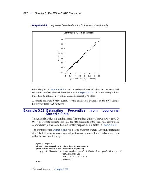
- Page 1848 and 1849: 370 Chapter 3. The UNIVARIATE Proc
- Page 1852 and 1853: 374 Chapter 3. The UNIVARIATE Proc
- Page 1854 and 1855: 376 Chapter 3. The UNIVARIATE Proc
- Page 1856 and 1857: 378 Chapter 3. The UNIVARIATE Proc
- Page 1858 and 1859: 380 Subject Index for estimating r
- Page 1860 and 1861: 382 Subject Index Kendall’s part
- Page 1862 and 1863: 384 Subject Index Mantel-Haenszel
- Page 1864 and 1865: 386 Subject Index
- Page 1866 and 1867: 388 Syntax Index CGRID= option HIS
- Page 1868 and 1869: 390 Syntax Index CONTGY option, 82
- Page 1870 and 1871: 392 Syntax Index LAMCR option OUTP
- Page 1872 and 1873: 394 Syntax Index PCTLAXIS option Q
- Page 1874 and 1875: 396 Syntax Index HMINOR= option, 2
- Page 1876: 398 Syntax Index VMINOR= option, 2