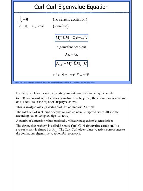
Curl-Curl-Eigenvalue Equation - Institut für Allgemeine ...

j ≡ 0 

S 

Curl-Curl-Eigenvalue Equation 

σ = 0, ε, µ real loss-free 

( no current excitation) 

( ) 

M CM 

Ce = ω e 

−1 2 

ε 

−1 

µ 

ε 

eigenvalue problem 

Ax = λx 

A = M CM C 

−1 

CC ε µ −1 

 

curl µ curl E = ω E 

−1 -1 2 

Ursula van Rienen, Universität Rostock, Institut für Allgemeine Elektrotechnik, AG Computational Electrodynamics 

For the special case where no exciting currents and no conducting materials 

(σ = 0) are present and all materials are loss-free (ε, µ real) the discrete wave equation 

of FIT resultss in the equation displayed above. 

This is an algebraic eigenvalue problem of the form Ax = λx. 

The solutions of such kind of equations are non-trivial eigenvalues x j ≠0 and the 

according real or complex eigenvalues λ j. 

A matrix of dimension n has maximally n linear independent eigensolutions. 

The eigenvalue problem is called discrete Curl-Curl-eigenvalue equation. It´s 

system matrix is denoted as A CC . The Curl-Curl-eigenvalues equation corresponds to 

the continuous eigenvalue equation for resonators.

Curl-Curl-Eigenvalue Equation 

1/2 

Use transformation e' = Mε 

e to derive an equation with 

symmetric system matrix 

 

 

M CM CM 

e' 

= e' 

1/2 −1/2 2 

ε −1 

ε 

ω 

µ 

system matrix 

1/2 −1/2 

A' 

= Mε 

ACC 

Mε 

= M CM CM 

= 

−1/2 −1/2 

ε 

µ −1 

ε 

−1/2 −1/2 −1/2 −1/2 

( Mε 

CM 

µ )( Mε 

CM 

µ ) 

T 

is symmetric 


Eigenvalues of both equations are the quadratic resonance frequencies ω 2 and the 

eigenvectors correspond each to the fields of the according resonator modes. 

Now we can study the properties of the FIT discretization by analyzing the algebraic 

properties of the system matrix A CC . 

In the actual form of the curl-curl-eigenvalue equation the matrix A CC is nonsymmetric. 

Yet, using the transformation given above for the electric grid voltage we receive the 

above formulation with real symmetric system matrix A’. The eigenvalues of A CC and 

A’ are identical.

Solution Space of Eigenvalue Problem 

λ = ω ≥ 0 ∀ λ = eigenvalue of A ' 

2 

i i i 

Consistency between mathematical model and physics is based upon 

T 

• Symmetry of the curl operators: C 

= C 

• Possibility to split the material operators: 

M = M M and M = M M 

ε 

1/2 1/2 1/2 1/2 

ε ε 

µ 

µ µ 

(real diagonal matrices with non-negative entries) 

Consider 

 

SC 

M C e = ω S 

M e = ω S 

d = 0 

2 2 

− 

µ 1 ε 

= 0 

 

⇒ either ω = 0 or Sd = 0 


The solutions of the discrete eigenvalue equation are not only of interest if we directly want to 

determine the oscillating modes in resonators but they also hold information about the behaviour 

of time-variable fields obtained by FIT-discretization. 

Using purely algebraic reasoning we can get information about the location of the eigenvalues: 

Because of it´s symmetry the matrix A’ (and thus also A CC ) has purely real eigenvalues. From it´s 

representation as product of two matrices transposed to each other it also follows that all 

eigenvalues are non-negative (A’ is positive semi-definite). 

Thus, also the eigenfrequencies ω j are real and non-negative. This corresponds to the physical 

property that loss-free resonators have real eigenfrequencies, only. 

This consistency between the mathematical model and physics is not self-evident. In this case it is 

based on the properties of 

• the symmetry of the discrete curl-operators of FIT, 

• the possibility to decompose the material operators because they are real diagonal matrices with 

non-negative entries. 

A further hint about the solution space of the eigenvalue problem can be obtained by the following 

physical consideration: If we multiply the curl-curl-eigenvalue equation from left by M ε and build 

the divergence next (multiplying from left the discrete divergence operator) we get the equation 

displayed above. This means that for all eigensolutions either the eigenfrequency ω or the 

divergence of the electric flux density have to vanish.


Solution space L 

can be decomposed: 

L= L 

S 

∪ L 

d 

2 2 

ω = 0 ω ≠0 

1. Subspace LS 

of electrostatic solutions with ω = 0 : 

 

i potential approach: E = − grad ϕ and e =− − 

Φ 

( 

) 

T 

( S ) 

T 

T 

i because of curl grad = 0 and CS 

= SC = 0 

 

 

⇒ curl E = 0 and Ce = 0 

S 

⇒ ω = 0 

 

i in general: div D ≠0 and 

S 

S 

S 

 

Sd ≠0 

S 

S 


The solution space L of the Curl-Curl-eigenvalue equation thus can be split into two disjoint 

subspaces: L S is the space of static solutions since it holds all eigensolutions λ=ω²=0. 

L d is the space of dynamic solutions which all have resonance frequencies above zero and thus 

correspond to harmonic oscillating fields. 

1. For the eigenvectors, i.e. the discrete field vectors, of both solution classes we find, using the 

properties of FIT – discretization: 

Electrostatic fields with ω=0: 

Such fields may be represented as gradient of a scalar potential. Because of curl grad=0 

the curl of the electric field and electric grid voltage is vanishing for these modes. Inserting this 

into the curl-curl-eigenvalue equations we obtain ω=0 as it should be. 

In a grid of N P points there exist about N p linear independent potential vectors ϕ and thus about N P 

linear independent static eigenmodes (ignoring points with fixed potential, as e.g. at the boundary). 

This means that the eigenvalue λ=0 is (about) N P -fold degenerate. 

In general, the potential distribution does not fulfil the Laplace equation such that we need to 

assume charges in the grid points for the existence of such solutions. This means that the 

divergence of the flux density is not equal to zero. 

Note: In problems with multiple conductors (structures with several disjoint ideal conductors), 

there exist also some modes with ω=0 which are divergence- and curl-free. We will not treat these 

cases here.


2. Subspace L of dynamic solutions with ω ≠ 0 : 

d 

i from Faraday's law we have: 

 

 

D5 ≠ 0 

 

curl E ≠0 and Ce ≠0 

d 

i from Ampere's law we get: 

1 1 

Dd = curl Hd and dd = Ch 

d 

jω 

jω 

i because of div curl = 0 and SC = 

0 we have 

 

 

div = 0 and Sd = 0 

D d d 

L= L 

S 

∪ L 

d 

2 2 

ω = 0 ω ≠ 0 

d 


Dynamic eigen-oscillations with ω≠0: According to Faraday´s induction law these modes 

possess a non- vanishing curl-contribution. 

The corresponding electric grid flux can be represented with help of Ampère´s law. Because of 

div curl=0 the dynamic modes are divergence – free. 

The exact separation of both subspaces with the provable curl-and divergence-freeness of the 

corresponding modes thus holds in the discrete case just because the matrix operators fulfil the 

necessary conditions. This is not at all self-evident and for some other discretization methods it 

does not hold! 

According to our previous considerations, the eigenvalue problem of dimension 3N P has the 

about N P – fold degenerated eigenvalue ω² = 0 and only about 2N p non-zero eigenvalues. 

The static modes, however, are meaningful solutions of Maxwell´s equations if and only if the 

charge distribution which results from div D s ≠ 0 is allowed for the solution domain. Since this 

is generally not the case as usually div D = 0 is assumed for harmonic problems our system 

matrix turns out to be „too large“ by about 1/3.


Im{ λ} 

N-fold eigenvalue 0 (static solutions) 

2 2 

2 Re 

ω 1 

ω 

2 

… ω 

{ λ} 

2 N 

smallest (non-zero) eigenvalue = fundamental oscillation 

Symmetry and positive semi-definiteness of A' 

⇒ orthogonality of the modes: 

 

e' ⋅ e' = 0 ∀i, j withλ ≠λ 

i j i j 

Orthogonality condition after back-transformation: 

 

ei⋅ Mεej = 0 and ei⋅ d 

j 

= 0 ( i ≠ j) 

4 x stored electric energy (non-zero only for i = j) 


Consequently, we should search for some transformation which reduces the dimension of the 

system matrix from 3N P to 2N P . Building in the discrete Gauss law for electricity with 

vanishing right hand side (no charges) would yield such a transformation but destroy the 

band structure of the matrix affording higher computational effort for it´s storage. 

Instead of this it is more elegant to control the static modes by a modified formulation of the 

wave equation and/or by specific algebraic solution methods which will be treated later. 

Another property of the solution of the Curl-Curl matrix A´. For two eigenvectors, each, of 

this matrix orthogonality holds if the corresponding eigenvalues are not equal to each other. 

Hence, orthogonality holds for all pairs of non-degenerated modes – also for each pair build 

by one dynamic and one static mode. For degenerated dynamic modes (with λ i =λ j ≠0) 

orthogonal linear combinations can always be found. 

After back-transformation from A` to A cc we obtain the orthogonality relation for dynamic 

eigenmodes given above. 

The scalar product of the vectors of electric grid voltage and electric grid flux formally 

corresponds to four times of the stored electric energy which is non-vanishing only if both 

vectors belong to the same field.

Grid Dispersion Equation 

Plane waves: 

j( t k r) 

E = E e ω − 

⋅ 

0 

2 

2 2 2 2 ω 

Dispersion equation: k = kx + ky + kz 

= 

2 

c 

With 

 

− jk⋅r 

− jk jk 

x x − y y − jkz 

z 

e = e e e 

− jk ∆x − jk ∆y 

− jkz 

∆z 

x y z 

x 

y 

T = e , T = e , T = e 

we find the phase factor 

by which the complex grid voltage is multiplied 

when the wave proceeds by one step size in x-, y- or z-direction 


Based on the discrete wave equation we will introduce next the so–called grid dispersion equation 

which allows for an extensive analysis of the properties of the Maxwell-Grid-Equation (MGE) for timedependant 

fields. 

The basis for the derivation is Fourier´s theorem according to which each wave may be represented as 

sum of elementary waves. In electrical engineering, this theorem is mainly applied to purely timedependant 

signals. It may also be applied to space-dependant electromagnetic fields: Then, elementary 

waves are fields which can be represented in space and time by harmonic functions, i.e. sine, cosine or 

the complex exponential function. Physically, these are just plane waves. 

In homogeneous space (vacuum) the plane waves are solution of (continuous) Maxwell´s equations for 

which the frequency ω or and the wave number k = |k| fulfil the dispersion equation. 

The idea of the following analysis is to check under which conditions plane waves exist on the grid, i.e. 

we can derive an according representation for the discrete field vectors which solve the MGE. First, we 

will study the time-harmonic case. 

In order to eliminate the influence of the boundary conditions we assume an indefinitely large Cartesian 

computation grid and equidistant step size in all three coordinate direction, i.e ∆u=∆v=∆w for all i=1,..., 

I, j=1,...,J, K=1, ..., K. Further, we assume constant material coefficients ε 0 , µ 0 and σ=0 (vacuum), 

Taking the continuous definition of a plane wave we impress the given electric field of the plane wave 

into the vector components of the electric grid voltage by evaluation of the corresponding path integral 

for each edge in the grid. Then, we find that the complex grid voltage has to be multiplied with the 

phase factors given above as the wave proceeds one grid step in x-, y- and z-direction, respectively. 

Thus, the complete discrete field vector can be explained by one voltage component per direction in 

space which will be denoted as shown here (a hat as sign for the wave amplitudes). As arbitrary origin 

for these discrete wave amplitudes we choose the three voltage components associated to some grid 

point n 0 (usual indexing).

e 

We have 

= E 

4 z 


Regard Faraday's induction law: 

 

b 

 

e = E 

⋅T 

1 x 

3 y z 

= B 

 

e 

= E 

1 y 

 

− jωb = e − e + e −e 

 

1 1 3 2 4 

= e1( 1− T z) + e4( − 1+ 

T y) 

x y( ) 

z z( y) 

 

e = E 

⋅ T 

2 z y 

z 

x y 

and − jω 

B = E 1− T + E − 1 + T for the wave amplitudes 


In the next step we will complete the time derivative of the magnetic flux component 

according to Faraday´s induction law for the corresponding grid areas. As we study 

the frequency domain, the time derivative is given by multiplication by јω. 

With the notations of the sketch we get the relations shown here.

Discrete induction law: 


 

 

⎛ 0 −( T 1) 

1 x 

x 

z − T y − ⎞⎛E 

⎞ ⎛B 

⎞ 

⎜ 

⎟⎜ 

⎟ ⎜ ⎟ 

T 1 0 ( 1) 

 

 

⎜ z 

− − T 

x 

− ⎟⎜Ey⎟=−jω 

⎜By⎟ 

⎜ ( T 1) 

1 0 

 

y 

T ⎟ 

⎝ 

− − 

x 

− 

⎠⎜E z ⎟ ⎜B 

z ⎟ 

⎝ ⎠ ⎝ ⎠ 

C 

⎛ ∆x 

⎞ 

⎜ 

⎟ 

⎛H 

 

x ⎞ ⎜ 

µ ∆y ∆z 

⎟ ⎛B 

x ⎞ 

⎜ ⎟ 

 

⎜ 

∆ y 

⎟ ⎜ ⎟ 

⇒ 

⎜H 

y⎟=⎜ ⎟ ⎜B 

y⎟ 

x 

, etc. 

µ z x 

H 

⎜ 

∆ ∆ 

⎟ 

⎜ 

z ⎟ ⎜B 

z⎟ 

⎝ ⎠ ⎜ 

∆z 

⎟ ⎝ ⎠ 

⎜ 

µ ∆x∆y⎟ 

⎝ 

⎠ 

∆ x=∆ 

homogeneous 

material 


M 

−1 

µ 

Thus, for all three directions in space, we obtain a mapping of the discrete induction 

law to the 3 x 3 system of equations as displayed above. 

So we have determined the magnetic flux components. Next, we can use the material 

equations to determine the wave amplitudes of the magnetic grid voltages. The 

discrete relation for the simple case of a homogeneous equidistant grid is given here.


Regard Ampere's law: 

1 

H 

x 

T 

y 

H y 

D z 

C 

 

1 

H 

T 

x 


y 

H x 

jω 

D 

Discrete law: 

−1 −1 

⎛ 0 −( 1−T z ) 1−T ⎞ 

y ⎛H 

 

x 

⎞ ⎛D 

x 

⎞ 

⎜ ⎟ ⎜ ⎟ ⎜ ⎟ 

⎜ −1 −1 

1−T 0 

z 

−( 1− T 

⎟ 

x ) ⎜ H y ⎟ = jω 

⎜ Dy 

⎟ 

⎜ ⎟ ⎜ −1 −1 

 

⎜−( 1−T 

) 1 0 H z D z 

y 

−T 

⎟⎜ ⎟ ⎟ ⎜ ⎟ 

x 

⎝ 

⎠⎝ ⎠ ⎝ ⎠ 

 

z 

= 

( 1 −1 ) 1 

( 1 

− 

T ) 

y 

H x T 

x 

H 

− − + − 

y 

Next, we will apply the discrete Ampère´s law to the corresponding dual area as 

shown in this sketch. The inverse phase factors in the resulting equation just have the 

effect of a displacement in negative coordinate direction. 

Again, we can summarize the equations for all three directions in space obtaining the 

system of equations given here. 

As we can easily verify the system matrices („curl operators“) again fulfil the relation 

that the one on the primary grid equals the Hermitian one the dual grid (Hermitian 

matrix = transposed plus conjugate complex).


Electric material matrix: 

⎛ ∆x 

⎞ 

⎜ 

⎟ 

⎛E 

 

x ⎞ ⎜ε 

∆y 

∆z 

⎟ ⎛D 

x ⎞ 

⎜ ⎟ 

 

⎜ ∆ y 

⎟ ⎜ ⎟ 

⎜E 

 

y⎟= ⎜ ⎟ ⎜D 

y⎟ 

ε z x 

E 

⎜ ∆ 

∆ 

⎜ 

z ⎟ 

⎟ 

⎜D 

z 

⎜ 

⎟ 

⎝ ⎠ ∆z 

⎟ ⎝ ⎠ 

⎜ 

ε ∆x∆y⎟ 

⎝ 

 

⎠ 

−1 

M 

ε 

Amplitude vector: 

⎛E 

⎞ 

x 

⎜ ⎟ 

e = ⎜E 

⎟ 

y 

⎜E 

⎟ 

⎝ 

z 

⎠ 


Finally , the electric material matrix is applied in order to transform the electric grid 

fluxes into grid voltages. 

Thus we have transformed all equations now to the three-dimensional space of wave 

amplitudes.

1 


The local Curl-Curl-wave equation 

−1 H −1 

2 

Mε 

C Mµ 

Ce 

= ω e 

has to hold for e 

! 

( ) ( ) 

jx 

Using the relation e = cos x + jsin x the lengthy solution 

finally yields 

λ = 0 (the static solution), 

λ 

λ 

c 

2 

2 

⎛ 

kx 

x ⎛ ⎛ky∆y⎞⎞ 

⎜ 

⎛ ⎛ ∆ ⎞⎞ sin 

sin 

⎛ ⎛kz∆z⎞⎞ 

⎜ ⎜ ⎟⎟ 

sin 

⎜ 

⎜ ⎜ ⎟ 

2 

⎟ 2 ⎜ ⎜ ⎟ 

2 

⎟ 

⎝ ⎠ ⎜ ⎝ ⎠⎟ 

⎝ ⎠ 

⎜ 

⎜ ⎟ ⎜ ⎟ 

∆x ⎜ ∆y ⎟ 

∆z 

⎜ 

⎜ 2 ⎟ ⎜ 2 ⎟ ⎜ 

⎝ ⎠ ⎝ 2 ⎟ 

⎜ 

⎝ ⎠ 

⎠ 

⎝ 

2 

2 

= 

3 

= + + 


2 

⎞ 

⎟ 

⎟ 

⎟ 

⎟ 

⎟ 

⎠ 

Sequentially applying the equations previously derived, a condition may be 

formulated under which the discrete plane wave fulfils the Maxwell-Grid-Equations 

as demanded before (thus justifying the approach used here). The electric amplitude 

vector has to fulfil the local Curl-Curl-Wave equation. 

This is an algebraic 3x3 eigenvalue equation for the electric amplitude vector with 

eigenvalue λ=ω². After some lengthy calculation and paying attention to the relation 

e jx = cos(x) + j sin (x) one eigenvalue λ 1 =0 and a double eigenvalue λ 2 = λ 3 as given 

above are found. The solution λ=ω²=0 is denoted as static solution. It is not regarded 

here. The two solutions λ 2,3 ≠0 describe the discrete waves, searched for. The 

corresponding two-dimensional space of their eigenvectors indicates the two 

polarisation directions of the plane wave.


The grid dispersion equation 

2 

2 

2 

⎛ ⎛ky∆y⎞⎞ 

z 

⎛ ⎛kx∆x⎞⎞ sin 

sin 

⎛ ⎛k ∆z⎞⎞ 

⎜ ⎜ ⎟ sin 

2 

⎟ ⎜ ⎜ ⎟⎟ 

2 ⎜ ⎜ ⎟ 

2 

⎟ ω 

⎜ ⎝ ⎠⎟ ⎛ ⎞ 

+ ⎜ ⎝ ⎠⎟ 

+ ⎜ ⎝ ⎠⎟ 

= 

x y z ⎜ ⎟ 

⎜ ∆ ⎟ ⎜ ∆ ⎟ 

∆ 

⎝ c ⎠ 

⎜ 2 ⎟ ⎜ 2 ⎟ ⎜ 2 ⎟ 

⎝ ⎠ ⎝ ⎠ ⎝ ⎠ 

2 

is the condition for the existence of the discrete waves belonging 

to the eigenvalues λ ≠ 0. 

2,3 


Finally, the condition for the existence of these waves is given as so-called grid 

dispersion equation. It connects the properties of the spatial discretization on the left 

hand side with the second time derivative of the wave equation which arises as factor 

–ω² in frequency domain (the negative sign is compensated by that in Faraday´s 

induction law). 

The grid dispersion equation fixes how plane waves propagate in the computational 

FIT-grid. For example, we can see that the propagation depends on the step size as 

well as on the propagation direction. Very important in that is that the grid dispersion 

equation tends to the analytic dispersion equation as we build the limits ∆x, ∆y, ∆z, 

∆t = 0. This is another proof of the convergence of FIT. 

Please note that we used some relevant assumptions on the grid for the derivation 

above: an equidistant discretization in all spatial directions, homogeneous material 

and no boundary conditions. Nevertheless, the grid dispersion equation is of great 

importance for the analysis of FIT´s properties as will get more obvious in the 

following chapters.

Solution of the Eigenvalue Equation 

−1 2 

Loss-free (real ε, σ=0): Mε 

CM 

µ − 1 

C e = ω e 

eliminate the N 

P 

solutions with λi 

= 0: 

 

dynamic modes with: div( ε E) = 0 

 

T 

grad div D = 0 − SSM 

ε 

e= 

0 

1/2 1/2 1/2 

Transformation e' = e: - M S T SM 

e' = 0 

M ε ε ε 

− 

( 

 

− T 

 

−1 

µ 

) 

1/2 1/2 1/2 1/2 2 

Mε CM CMε + Mε S SMε e 

' = ω e' 

 

-1 1 2 

ε µ ε E = ω E 

− 

( curl curl- grad div ) 

2 

"Nabla-Squared Eigenvalue Eq." (curl curl - grad div = - ∇ ) 


The eigenvalue equation of FIT for time-harmonic fields in closed structures (resonators) has 

been formulated in the previous chapter. For the loss-free case (real material coefficients and 

vanishing conductivity) it is repeated here. 

Usually, the dynamic modes with the smallest non-zero eigenvalues λ=ω²≠0 are of technical 

interest. As previously found, in this regime the spectrum of the system matrix is determined 

by the multiple degenerated eigenvalue λ=0. Since this situation poses great numerical 

difficulties for most eigenvalue solvers we will derive an alternative formulation in the 

sequel. 

Solution methods which search for the smallest eigenvalues and the corresponding 

eigenvectors of a matrix would first compute all eigenvalues with ω²=0 and only then they 

could compute the fundamental mode as second-smallest eigenvalue. 

Therefore, our goal is to eliminate the N P -fold eigenvalue zero in the matrix A CC. 

For all dynamic modes searched for we have div (ε E)=0 and the corresponding discrete 

equation in grid space. Now we multiply the discrete equation from left with the discrete 

gradient operator (continuously, we build the gradient of the left hand side.) 

Replacing now the electric grid voltage by its transformed form we find a symmetric form of 

the last equation. 

Now we subtract this equation from the Curl-Curl-eigenvalue equation. The resulting 

equation is given in the original and in its symmetric form. Also the continuous form is given.


„Ghostmodes“ in inhomogeneous waveguide 


Because of the vector identity curl curl – grad div = -∇² this equation is also denoted as Nabla- 

Squared-Eigenvalue equation. Only the dynamic modes are searched for, but not the static fields 

(with div D≠0) fulfil this equation. 

Since the solution manifold has to be preserved we will study next which solutions replace the 

static solutions. 

One can show that, again, we obtain two types of solution: 

1. eigensolutions with ω² >0, div D=0 and curl E≠0: 

These are the modes searched for. (Here, we also count the modes in 

multiple conductor systems for which still holds: ω²=0, div D=0, curl 

E=0) 

2. eigensolutions with ω² >0, div D≠0, curl E=0: 

These modes obey to the equation - grad div E=ω² ω µ E and therefore they are no 

physically meaningful solutions. 

The elimination of the static solutions thus leads to the appearance of unphysical solutions, the socalled 

„Ghost Modes“. They always appear when we solve the Curl-Curl-eigenvalue equation in 

the latter form. After the solution of the eigenvalue problem we thus need to distinguish the ghost 

modes from the physical dynamic modes.

Solution of the Eigenvalue Equation (C‘ted) 

„Ghostmodes“ in inhomogeneous waveguide 


Numerical approaches and discretization methods which cannot fulfil the relation div 

curl=0 on the grid space have no straightforward possibility to distinguish the two 

solution types. They often apply the so-called penalty method where the grad divterm 

in the eigenvalue equation is weighted by some factor p (penalty factor). After 

multiple solution with different values of p the correct (physical) eigensolutions can 

be distinguished because they do not show any dependence on p. 

With FIT this effort of multiple solution of the eigenvalue problem is not necessary 

since the product of the div and curl operator vanishes and thus it is sufficient to 

apply the dual divergence operator to the electric grid flux to distinguish the two types 

of solution.

Memory Usage 

Example: 

mesh points: 

N = 

P 

6 

10 (double precision: 8 bytes/number) 

FIT: 39 bands of entries 

N P 

(21 have to be stored, symmetry) 

⇒ 170 MB (+ some add. vectors) 

no band structure: 

fill-in-entries by solver (still symmetric!) 

⇒ 

0 .6 

2 

13 

.5 (3N P 

) = 3 ∗10 Byte 


Our eigenvalue problem has the dimension N=3 N P and thus also N eigensolutions. The 

number N P of grid points may be very large in some applications (up to a few millions) which 

involves that a complete solution is generally hardly possible. 

In the following, we will describe an iteration method for the solution of such kind of 

eigenvalue problems. In the practically interesting case of only a few 10-100 eigenvalues 

searched for, this method provides good results with acceptable effort. 

All methods described here exploit the fact that the system matrix is very large but sparse: In 

the iterative solution of the eigenvalue problem only so-called „matrix-vector-operations“ are 

used for which the matrix pattern can directly be exploited for an efficient implementation. In 

general, methods which afford a decomposition of the matrix should not be applied since they 

destroy the band structure. 

As example let us assume a computational grid of N P = 10 6 grid points. According to the 

previously found structure the Curl-Curl-System matrix has 39 bands of length N P where 

only 21 of those have to be stored because of symmetry reasons. For a double-precision 

calculation we need 8 Byte per floating point number which yields a storage requirement of 

about 170 MB. Additionally, we need to store some auxiliary vectors (depends on the solution 

method). This is easily affordable on modern PC´s or workstations. 

Yet, if we would loose our band structure and would need to store the complete matrix 

(because of fill-ins produced by the solution method) we would end up with 0.5* (3N P )² = 4.5 

* 10 12 numbers or 3.6 * 10 13 Byte (still for a symmetric matrix!)

von Mises-Iteration 

x 

A 

( 0) 

is real symmetric: 

( ) 1 2 3 N 

Ax = λx dim A = N λ > λ ≥ λ ≥… ≥ λ 

filled with random numbers, expressed as linear combination of e: 

x 

( 0) 

N 

= ∑αie 

i= 

1 

i 

i 

Iteration scheme x 

( v) ( v−1) 

= Ax 

leads to: 

⎡ 

⎤ 

v 

N 

⎢ 

N 

( v) 

v v 

⎛λ 

⎞ ⎥ 

i 

x = ∑αλ i i 

ei = λ1 ⎢α1e1+ ∑⎜ ⎟ αiei⎥ 

i= 1 ⎢ i= 

2⎝λ1 

⎠ ⎥ 

⎢ 

 

⎣ 

→0forv→∞ 

⎥⎦ 


As introduction we will study the von Mises method, also called „power iteration“, 

to determine a specific solution for an eigenvalue problem of the form 

Ax = λx, dim (A) = N. 

We assume that the matrix A is real symmetric with eigenvalues 

| λ 1 | > | λ 2 | ≥ | λ 3 | ≥ ... ≥ | λ N |. 

We search for the (uniquely defined) eigenvalue λ 1 with large absolute value and 

the corresponding eigenvector x 1 . 

We start with an initial vector x (0) filled with random numbers. Since the 

eigenvectors of A build a complete orthogonal system we can represent x (0) as 

linear combination of eigenvectors e 1 , ..., e N as displayed above. 

Now we use the iteration scheme 

x (v) = Ax (v-1) 

And get the expression given above. 

The iteration converges against the eigenvector e 1 belonging to the eigenvalue λ 1 

with larges absolute value.

Eigenvalue Solver 

Rayleigh-quotient: 

( v) ( v) 

( v) 

x ⋅ Ax ⎛ ⎛ λ 

( ) 

ε 

⎞ 

R x = = λ 

( v) ( v) 

∞ 

⎜ 

∞+Ο⎜ ⎟ 

x ⋅ x 

⎝λ 

⎝ 

∞ ⎠ 

λ =R 

1 

( v) 

( x ) 

εv+∞ 

⎞ 

⎟ 

⎠ 

Normalization during iteration: 

( v) ( v−1) ( v) 

x = Ax , x = 

x 

x 

( v) 

( v) 


A very good estimation of this eigenvalue can be obtained by the Rayleighquotient 

given above. 

In order to avoid a fast increase of the vector components of eigenvalues with | 

λ i | > 1 during the iteration a normalization is carried out after each step of the 

von Mises- iteration. 

The vector norm used in the normalization is arbitrary.

Iteration Scheme 

1. Choose randomly filled vector 

( 0) 

x 

2. For ν=1,2,3,… build: 

( v) ( v− 

) 

( v) 

( v) 

( v) 

1 , 

3. Build Rayleigh quotient 

x 

x 

= Ax 

= 

x 

x 

λ =R 

( ) 

( ) 

1 

x v 

4. Repeat step 2-3 until the desired accuracy is reached 


The complete iteration is given above.

Spectral Shift 

The von Mises-iteration yields the eigenvector with largest eigenvalue. 

Often the eigenvector corresponding to the smallest eigenvalue is 

of special interest. 

Define A ' with: 

( λ s) ( ) 

Ax ' = Ax+ sx= + x x: Eigenvector of A 

System matrix A' with eigenvectors x, but eigenvalues are shifted: 

λ' 

= λ + s 


With the von Mises-iteration in the previous form only the maximal eigenvalue (absolute value) 

of a matrix and it´s corresponding eigenvector can be found. Yet, for practical applications just 

the smallest eigenvalues are of interest (the fundamental mode of a cavity resonator, e.g.). 

By help of a spectral shift the same method can also be used to compute the smallest 

eigenvalues of a matrix. To do so the iteration is carried out with the slightly modified matrix 

A‘ = A + sI which has the same eigenvectors as A but shifted eigenvalues λ‘= λ + s as 

the above given consideration shows. 

If the spectrum of A is known in a good approximation the spectral shift s can now be chosen 

such that the smallest eigenvalue λ k 

searched for gets the eigenvalue λ k ’ of A’ with largest 

absolute value and can thus be computed with the von Mises-iteration. However, with this 

procedure we have to face the problem that numerical cancellation might occur for finite 

computational precision in the final back-transformation λ k = λ k 

’- s. 

Another problem arises in case that an eigenvalue λ i 

matrix A’ will get singular then. 

is chosen for s since the transformed

Inverse Iteration 

−1 

Iteration of : 

A 

1 

= λ ⇒ = 

λ 

−1 

Ax x A x x 

In connection with spectral shift, each arbitrary 

eigenvalue may be computed: 

− 

( s ) 1 

A' 

= A− 

I 


If we take the inverse A -1 instead of A for our iteration the algorithm will converge 

against that eigenvalue of A with smallest absolute value because of 

Ax = λx ⇒ A -1 x = 1/ λ · x . 

But this advantage has to be paid by the much higher numerical effort of the inverse 

iteration: Either we have to build A -1 once a priori or we have to solve a linear system 

in each step. 

Nevertheless this method is often used since in connection with a spectral shift A’ = 

(A – S I) -1 each arbitrary eigenvalue of the spectrum may be computed.

Sub-Space-Iteration 

Very large, sparse matrix A, 

dim( A) = N, λ ≥ 0 real 

Look for basis vectors (not necessarily eigenvectors): 

( j) 

p 

∑ 

i= 

1 

j 

i 

i 

( 1 ) 

v = c e j = … p 

Eliminate all components of unwanted eigenvectors 

by iteration with 

( = 1… 

) 

A− 

r k n 

I k 


The sub-space iteration described in the following simultaneously computes several 

eigenvectors in each application. The basic idea is to compute several basis vectors 

during the iteration which together span a subspace of the complete solution space 

where the searched eigensolution lie in this subspace. 

Given a very large sparse real matrix A of dimension N x N with eigenvalues λ. 

Further we assume that all eigenvalues are real and non-negative 

( symmetric positive semi-definite matrix.) 

We are searching for the „first“ p eigensolution, i.e. those eigenvectors belonging to 

the p smallest eigenvalues ( with p=10; ....100)

Sub-Space Iteration 

The computation of the eigensolution is done in two steps: 

1. The p so-called basis vectors spanning the sub-space 

containing the eigenvectors, searched for, are computed. 

2. Using these basis vectors, the given N x N- eigenvalue 

problem is transformed into a smaller eigenvalue problem of 

dimension p x p. The spectrum of this smaller problem holds 

the searched eigenvectors and can be solved by a direct 

solution method. 


The computation of the eigensolution is done in two steps: 

1. The p so-called basis vectors spanning the sub-space containing the eigenvectors, 

searched for, are computed. 

2. Using these basis vectors, the given N x N- eigenvalue problem is transformed into 

a smaller eigenvalue problem of dimension p x p. the spectrum of this smaller 

problem holds the searched eigenvectors and can be solved by a direct solution 

method.

Sub-Space-Iteration 

0 

( r ) 

( r ) 

( 0) 

( 0) 

( 0) 

i= 

1 

( λ r) 

1 1 i i 1 i 

i= 

1 

n N n 

( λ r ) 

n k i i k i 

k= 1 i= 1 k= 

1 

N 

v = v = α e 

v = A− I v = α − e 

∏ 

v = A− I v = α − e 

= 

∑ 

N 

∑ 

∑ ∏ 

N 

∑ 

i= 

1 

i 

α P 

i 

( λ ) 

e 

i n i i 

( λ) = ( λ− 

) 

with polynomial of the order n: 

P r 

n 

n 

∏ 

k = 1 

k 


Thus we need to search for a set of basis vector, i.e. linear independent vectors v (j) 

which each can be represented as linear combination of all searched eigenvectors e j 

(i 

=1…p). (The vectors v (j) themselves need not to be eigenvectors of A.) 

Then, an arbitrary vector of this sub-space of p basis vectors does not hold any 

component of the remaining (not interesting) eigenvectors e i 

with i = p+1, …, 

N. 

Therefore, our goal in the computation of the basis vectors is to eliminate all 

components of these undesired eigenvectors starting with some arbitrary initial vector 

v (0) . 

This can be reached by repeated multiplication of the initial vector v (0) with the 

matrix 

A - r k 

I (k = 1, …, n). 

The spectral shift by r k 

can vary now in each iteration step. 

Analogous to the procedure in the von Mises-iteration we receive the representation 

given above with a polynomial P n 

of order n, i.e. the number of iterations.


20 

15 

10 

5 

0 

−5 

Suppressed domain 

0 1 2 3 4 5 

Tschebyscheff polynomial of degree n=20, shifted and scaled 


We can interpret the real values r i 

as zeros of the polynomial P n 

. We see that the 

components of the single eigenvectors e i 

contained in the initial vector v (0) are 

suppressed or “accelerated” according to the polynomial value P n 

(λ i 

). 

Now, the so-called accelerating polynomial and it´s zeros r k , respectively, may be 

chosen such that after sufficiently long iteration the basis vectors only hold 

components of the searched eigenvectors. 

Appropriate are e.g. the Tschebyscheff polynomials which are well-known from 

filtering techniques. Their degree n is fitted to the prescribed accuracy conditions.

Curl-Curl-Eigenvalue Equation - Institut für Allgemeine ...

Create successful ePaper yourself

Delete template?

Save as template?