Institut für Allgemeine Elektrotechnik, Uni Rostock - Universität ...

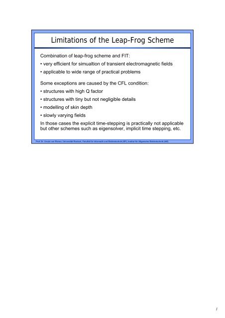
Limitations of the Leap-Frog Scheme 

Combination of leap-frog scheme and FIT: 

• very efficient for simualtion of transient electromagnetic fields 

• applicable to wide range of practical problems 

Some exceptions are caused by the CFL condition: 

• structures with high Q factor 

• structures with tiny but not negligible details 

• modelling of skin depth 

• slowly varying fields 

In those cases the explicit time-stepping is practically not applicable 

but other schemes such as eigensolver, implicit time stepping, etc. 

Prof. Dr. Ursula van Rienen, Universität Rostock, Fakultät für Informatik und Elektrotechnik (IEF), Institut für Allgemeine Elektrotechnik (IAE) 

1


What is the Q factor? 

Q factor plays an important role for resonators, filters, etc. 

It gives the relation between stored energy and the power loss in 

the walls: 

ωW 

Q = P 

with the stored energy of the time-harmonic field in volume V 

v 

1 1 

W = εr 

* dV μr 

* dV 

2∫ 

E⋅ E = ⋅ 

2∫ 

H H 

V 

and the power loss, i.e. Ohmic losses by wall currents 

1 J⋅ 

J* 1 ωμ 

Pv = dV 

t t 

* dA 

2∫ 

= ⋅ 

σ 2 2σ∫H 

H 

V 


2

TESLA Cavity 

Photo/graphic: 

DESY Hamburg 

www.linearcollider.org 

ILC will use 16,000 superconducting cavities to 

accelerate electrons and positrons to 99.9999999998 

percent of the speed of light. 


3


1. Structures with high quality factor (resonators, filter, ...): 

ω ⋅ Ws 

frequency × stored energy 

Quality factor Q is defined as Q = = 

Pv 

losses 

⎧long decay time of resonant oscillation 

High Q → ⎨ 

⎩ long rise time 

of 

the fields 

4 

Example: resonator with copper walls typically has Q ≈7 ⋅10 

Q 

4 

⇒ only after ≈10 periods the stored energy decayed to 

2π 

about 37% of it's initial value 

For a typical discretization and 20 time 

steps per period this means 

5 

that more than 10 time integrations would be necessary 

Long 

computation time 

in time domain → usually frequency domain 

is chosen in such cases 


4


2. Modelling of small geometrical details: 

Functions of the grid: i) sampling the wave in space and time 

ii) map the material distribution to discrete space 

Difficulty if ratio of wavelength to geometrical detail is large: 

over-sampling 

of the wave in space and time 

Example : Plane wave of 30 MHz (wavelength ≈ 10 m) incident 

on perfect conductor with surface details in 

mm-range 

Δ x = Δ y = Δz ≈ Δt 

≈ ⋅ 

−12 

For 1mm we get 2 10 s from CFL 

−8 

For a period of 3,3 10 s we would need more 

T 

≈ 

than 17,000 time steps per period! 

This leads to an enormous computational effort why subgrids or 

a 

conformal approach are used then. 

⋅ 


5


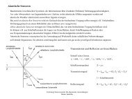
3. Skin depth modelling: 

Skin depth of good conductors wave length in free space 

To sample the exponential field decay inside the conductors 

a sufficiently fine grid is needed which in turn leads to extremely 

small time steps and thus to a strong loss in efficiency 

Solution: special layer models 

for skin depth without discretization 


6


4. Slowly varying fields ("low-frequency fields", Quasistatics): 

wavelength 

dimension 

(e.g. motors or generators at 50 Hz) 

i incident field in conductor has to be modelled by discretization 

i matei 

r als often non-linear 

Example: Copper cube of 10 cm side length inside of cubic 

grid of d = 1m side length and uniform step size of 5 mm; 

7 

conductivity 5.8 ⋅10 S/m, applied alternating current of 50 Hz 

⇒ skin depth of δ = 2 / ( ωµ 

κ) 

≈1cm while vacuum wave 

6 

length is λ = c / f ≈ 6 ⋅10 m 1 m (grid size). 

For the time integration of one period T = 0.02 s the maximal 

−12 9 

stable time step is Δtmax 

≈9.6 ⋅10 s affording 2⋅10 t 

Solution: 

Implicite time integration scheme 


ime steps! 

7

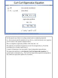
Initial Value Problem of Time Domain 

For stability studies we regard a single system of differential equations: 

d 

y= Ay+ q, y( 0 ) 

= y 

t= 

t 

dt 

representing the discrete Faraday's and Ampere's law. 

initial value problem of the time domain formulation of FIT with: 

 

⎛ 

0 

−1 

h⎞ 

⎛ −M 

C⎞ 

µ 

solution vector: y= ⎜ 

⎟, system matrix: A= ⎜ −1 −1 

⎝e⎠ ⎟ 

⎝Mε C 

Mε Mσ 

⎠ 

( 0) 

source vector: 

⎛ 0 ⎞ 

q= , initial value: 

y 

⎜ −1 

− ⎟ 

⎝ Mε 

jS 

⎠ 

( t = t ) 

0 

= y 

( 0) 


8

Properties of the System Matrix 

( σ = ⇒ M = ) 

In the loss-free case 0 0 

similarity transformation 

A' 

−1/2 1/2 

⎛ ⎞ ⎛ ⎞ 

−1 −1 

µ µ 

= ⎜ ⎟ A ⎜ ⎟ 

to transform A to the real skew-symmetric matrix A' 

⎛ 

A' 

= ⎜ 

⎜M 

⎝ 

M 0 M 0 

⎜ 1/2 ⎟ ⎜ −1/2 

⎟ 

⎝ 0 Mε 

⎠ ⎝ 0 Mε 

⎠ 

0 −M CM 

−1/2 

T 1/2 

ε 

CM 0 

1 

µ − 

with identical spectrum. 

1/2 −1/2 

−1 

µ ε 

⎞ 

⎟ 

⎟ 

⎠ 

σ 

we may apply the 


9


Properties of the system matrix: 

i All eigenvalues of A lie on the imaginary axis. 

λ A ,i 

They are either 0 or complex-conjugate in pairs. 

i A complete basis of eigenvectors exists. 

Eigenvectors of different eigenvalues are orthogonal. 

A simple estimate for the absolute largest eigenvalue ω 

yields ω 

max 

≤ A' for any arbitrary matrix norm. 

= max λ 

max A,i 

Example: µ ≡ µ , ε ≡ε 

, Δ u = Δ v = Δ w = Δ yields : 

0 0 

1 ⎛0 −C⎞ 

4c 

A' = ⎜ ⎟ ⇒ A' = A' 

= 

∞ 1 

µ 

0ε 

Δ 

0Δ ⎝C 0 ⎠ 

0 


10


Generally, the following estimate may be used: 

Cell i : Δ u ×Δ v ×Δw with ε , µ 

ω 

max 

≤ 

i ì i i i 

2 1 1 1 

ωi 

= + + 

ε µ Δu Δv Δw 

max 

i 

( ω ) 

i 

i 

2 2 2 

i i i 

In the lossy case similar estimates are possible: 

{ i} 

{ } 

− MM ≤ Re ≤0 

−1 

σ ε 

λ 

−ω ≤ Im λ ≤ω 

max i max 


11

Recursive Time Integration Method 

Formal solution of the initial value problem: 

() 

( 0) 

( ( ) ( )) 

y t = y + Ay t' + q t' dt' 


∫ 

t 

t 

0 

Exact solution of these large systems (complete decomposition in 

eigenvector basis or exponential matrix of A) not possible in 

practical applications. Therefore: recursive solution. We distinguish: 

i explicite 

and implicite recursion, depending on the formula for a 

new value: explicite or affording to solve an equation or a system 

of equations 

i single and multi ple step method s, depending 

on the number of 

old values taken into account. Linear single step methods may be 

( m + 1) ( m ) ( m ) 

written as y = Gy + q with the recursion matrix G. 

12

Stability 

Stability is one of the most important properties of a numerical 

integration scheme. 

( Δt) 

The linear recursion operator G depends on Δt. 

Several slightly different definitions can be found for the term "stability" , 

the following plays an important role in convergence analysis. 

Definition by Lax-Richtmeyer: 

( m+ 

) 

Δ 

( 

t0 

> 

) ( m 

t 

) 1 

( t) 


( m) 

A recursion y = G Δ y is stable 

if a constant C and 

a value 0 exist for each (fixed) value T such that 

holds. 

( ) ( m) 

G Δ ≤C 

∀m⋅Δt ≤T and Δt < Δt 

i.e. G Δt remains bounded for Δt →0 and constant T ( m →∞). 

0 

13

A sufficient stability 

condition is 

G 

( Δt 

) ≤1 

( ∀Δt 

) 

since this also involves 

m 

( t) G( t) 

G Δ ≤ Δ ≤1. 

Then, for y 

y 

Stability 

( Δt 

) ≤ ( ∀Δt 

) 

G( Δt 

) 

A sufficient condition for G 1 

λ 

G 

≤ 1 

( m) 

m 

we get 

( m) ( m−1) m ( 0) m ( 0) ( 0) 

= Gy = … = G y ≤ G ⋅ y ≤ 

i.e. the solution norm stays bounded (note: no excitation assumed!) 

for all eigenvalues of 

different recursion methods w.r.t. their stabilty. 

i 

y 

, 

is 

. It may be used to study 


14

Stability of Some Recursion Methods 

The three most simple time integration schemes are based on 

approximating the time derivative by: 

1. forward difference quotient: 

2. backward difference quotient: 

3. central difference quotient: 

(constant time step Δt) 

( ) 

f 

t 

0 

( + Δt ) − f ( t ) 

0 0 

f ( t0) 

f t0 

f − ( − Δt 

) 

( t ) ≈ 

0 

( ) 

f 

t 

0 

f t 

≈ 

f t 

≈ 

Δt 

Δt 

( + Δt 

/2) − f ( t −Δt 

/2) 

0 0 

Δt 


15

y 

⇒ 

( m+ 

1) ( m) 

− y 

Δt 

Forward Difference Quotient 

( m) ( m) 

= Ay + q 

( m+ 

1) ( m) ( m) 

( m+ 

1) 

explicite 

recursion formula for y : 

y =Δ tA+ I y +Δt 

q 

 

G 

(no inversion, just matrix-vector multiplications) 

In loss-free case ( Mσ =0) A has purely imaginary eigenvalues λ = jω 

for it's eigenvectors y ⇒ eigenvalues of G: 

( t ) ( Δt⋅ jω 

+ ) 

Gyi = Δ A+ I yi = 

i 

1 yi. 

 

Each eigenvalue λ 

Ai , 

i 

λ 

Gi , 

≠ 0 leads to an eigenvalue λ 

⇒ independently of Δt, the 

forward difference quotient is never stable! 


Gi , 

> 1 

A, 

i 

i 

16

Forward Difference Quotient 

Im 

( λ G ) ( ωΔt) max 

1 

Eigenvalues always lay outside of 

the (shaded) stability area with 

λ ≤ 1. 

G 

( ω Δ t) = 0 

1 

Re 

( λ ) 

G 

− 

( ωΔt) max 


17

Backward-Difference Quotient 

y 

( m+ 

1) ( m) 

− y 

Δt 

( ) ( ) 

( m+ 1) ( m+ 

1) 

= Ay + q 

( −Δt 

A+ 

I) 

( ) ( ) 

( + t ) 

m+ 1 m+ 1 − 1 m m+ 

1 

Resolving for y : y = y Δ q 

 

yields an implicit scheme, i.e. either we need to compute an inverse 

or solve a linear system (more efficient if A is sparse). 

For the eigenvalues of G we get 

−1 

1 

Gy = ( −Δ t A + I) 

y = y 

−Δ ⋅ + 

 

i i i 

t λAi 

, 

jωi 

1 

⇒ no eigenvalues of G are larger than 1, 

i.e. the backward difference quotient is stabl e for any arbitrary Δt. 

G 

λ 

Gi , 


18

Backward-Difference Quotient 

Im 

( λ G ) ( ωΔt) max 

1 

Eigenvalues always lay inside of 

( ω Δ t) = 0 

the (shaded) stability area with λ ≤ 1. 

( ) 

1 

Yet, accuracy depends Reon 

λGΔ 

t 

why a time step control is necessary. 

G 

Im 

( λ ) 

G 

1 

( ωΔ t) max 

( ωΔ t) = 0 

−( ωΔ t) max 

Re( λG) 

1 

− 

( ωΔt) max 


19

Central Difference Quotient 

In the loss-free case ( = 

Mσ 0) and allocating h in t + 0 

m ⋅Δ t, 

⎛ 1 ⎞ 

e in t0 

+ ⎜m+ t the leap-frog scheme results from the central 

2 

⎟⋅Δ 

⎝ ⎠ 

difference quotient which we will study now as single step scheme: 

d ⎛ 0 A12 

⎞ 

y = ⎜ ⎟ y+ 

q 

dt ⎝A21 

0 ⎠ 

−1 

with A12 =− M −1 

C, 

A 

µ 

21 

= Mε 

C 

 

⎛h⎞ 

⎛ 0 ⎞ 

and the vectors y = ⎜ 

⎟, q=⎜ 

. 

⎜ −1 

⎝e⎠ − ⎟ 

⎝ Mε 

jS 

⎠ 


20

Leap-Frog Update Equations 

 

( m 

( ) 

 

) 

m+ 1 ( m) ⎛ 

( m+ 

1/2) ( m) 

h ⎞ 

h = h +Δt⋅ A12e y =⎜ ⎜ ( m+ 

1/2) 

⎟ 

⎝ e ⎠ 

( m+ 3/2) ( m+ 1/2) ( m+ 1) 

−1 

( m+ 

1) 

e = e +Δt⋅A21h −Δt⋅Mε 

jS 

( ) 

( ) ( ) 

 

= e +Δ ⋅ A h +Δ ⋅A e −Δ ⋅M j 

 

 

= +Δ ⋅ +Δ ⋅ −Δ ⋅ 

 

−1 

( ) 

( ) ε S 

m+ 1/2 m m+ 1/2 m+ 

1 

t 

21 

t 

12 

t 

( 2 ( m+ 1/2) ( m) − ( 1) 

) 1 m+ 

I t A21A12 e t A21h t Mε 

jS 

which yields 

 

( m 

⎛ ) 

0 

( m+ 

1) ( m) ( m) ( m) 

h ⎞ ⎛ 

⎞ 

( m) 

y = G y + q with y = =⎜ ⎜ q 

( m+ 1/2) 

⎟ ⎜ 

 

−1 

( m+ 

1) 

Δt 

⎟ 

⎝ e ⎠ ⎝ Mε 

jS 

⎠ 

⎛ I ΔtA 

⎞ 

G = ⎜ ⎟ 

⎝ 

⎠ 

12 

and the recursion matrix . 

2 

Δ tA21 I+Δt 

A21A12 


21

Central Difference Quotient (Leap Frog) 

To determine the eigenvalues of G we first study the 

eigenvalue equation of the system matrix A : 

 

⎛h 

⎞ 

i 

Ayi = λA , i 

yi with yi 

=⎜ ⎜ 

⎟ 

⎝ei 

⎠ 

 

 

→ A e = λ h and A h = λ e 

12 i A, i i 21 i A, 

i i 

 

⎛ h ⎞ 

i 

Let y' i 

= ⎜ 

be an eigenvalue of . 

α ⎟ 

G 

⎝ ei 

⎠ 

Multiply inserting the last 2 equations yields 

 

⎛ 

i ( 1 α t λA, 

i) 

⎞ 

⎛ ⎞ 

h + Δ ⋅ 

hi 

G 

⎜ ⎟ 

⎜ 

1 

2 

. 

− 

α ⎟ 

= 

 

i α 

i ( 1+ α Δt⋅ λA , i 

+ ( Δt⋅λ 

⎝ e ⎠ ⎜ e 

A, 

i) 

) ⎟ 

⎝ 

⎠ 


22

Central Difference Quotient 

⇒ y ' is an eigenvalue of G with Gy ' = λ y ' ⇔ 

i i G, 

i i 

( ) 

1+ α Δt⋅ λ = 1 + α Δt⋅ λ + Δt⋅λ holds for α. 

− 1 

Ai , Ai , Ai , 

λ 

G, 

i−1 

Inserting λG, i= 1+ α Δt 

⋅λA , i 

⇒ α = Δ t ⋅ λ 

yields 

( t ) 

λ − λ 2+Δ ⋅ λ + 1= 

0 

or 

2 2 2 

G, i G, i A, 

i 

( t λ 

, ) 

⎛ 

Ai ( t λ 

Ai , ) 

2 2 

2+ Δ ⋅ 2+ Δ ⋅ ⎞ 

λ 

G, 

i 

= ± ⎜ 

⎟ −1 

2 ⎜ 2 ⎟ 

⎝ 

⎠ 

describing the relation between the eigenvalues of A and G. 


2 

2 

Ai , 

23


Regard the loss-free case, i.e. σ = 0, where λ A,i = j ω i : 

λ 

Gi , 

( t λ 

, ) 

⎛ 

Ai ( t λ 

Ai , ) 

2 2 

2+ Δ ⋅ 2+ Δ ⋅ ⎞ 

= ± ⎜ 

⎟ −1 

2 ⎜ 2 ⎟ 

⎝ 

⎠ 

( jω 

t) ⎛ ( jω 

t) 

2 2 

2+ i 

⋅Δ 2+ ⎞ 

i 

⋅Δ 

= ± −1 

2 ⎜ 2 ⎟ 

⎝ 

⎠ 

2 

2 

Dependingon thesignwegettwobranchesof theOrtskurve 

bothstartingatλ G = 1 which results from ωΔt = 0 

Each branch runs in one half of unit circle 

ending at λ G = - 1 which corresponds to | ωΔt | = 2 


24


Im 

( λ ) 

G 

1 

" + " 

ω Δ t = 

0 

( ω t) max 

± Δ 

" − " 

( ω t) max 

± Δ 

" + " 

1 

Re 

( λ ) 

G 

ω Δ t = 

2 

" − " 

Dependingon thesignwegettwobranchesof theOrtskurve 

•bothstartingatλ G = 1 which results from ωΔt = 0 

• each branch runs in one half of unit circle 

• ending at λ G = - 1 which corresponds to | ωΔt | = 2 


25


Im 

( λ ) 

G 

1 

" + " 

ω Δ t = 

0 

( ω t) max 

± Δ 

" − " 

( ω t) max 

± Δ 

" + " 

1 

Re 

( λ ) 

G 

ω Δ t = 

2 

" − " 

• λ G is purely real for larger values of ωΔt 

• The positive branch approaches zero 

• The negative branch approaches -∞ 


26


Im 

( λ ) 

G 

1 

" + " 

ω Δ t = 

0 

( ω t) max 

± Δ 

" − " 

( ω t) max 

± Δ 

" + " 

1 

Re 

( λ ) 

G 

ω Δ t = 

2 

" − " 

Stability conditions demands: max λ ≤ 1 

From this one can derive a condition for Δt 

which insures 

that ω Δt 

≤ 2 : 

i 

2 

Δt 

≤ Δ t = with ω = max λ 

ω 


Gi , 

max max A, 

i 

max 

27


⎛ 2 1 1 1 

Inserting the estimate ωmax 

≤ max = max 

+ + 

⎜ 

⎝ ε u v w 

iµ 

Δ Δ Δ 

i 

for the absolute largest eigenvalue yields again 

⎧ 

⎫ 

1 

⎪ 

⎪ 

Δt ≤Δt max 

≈min ⎨ εi µ 

i 

⋅ 

, 

i 

1 1 1 

⎬ 

⎪ 

+ + ⎪ 

2 2 2 

⎪⎩ 

Δui Δvi Δwi 

⎪⎭ 

i.e. the Courant-Friedrichs-Levy condition. 

( ωi 

) ⎜ 

2 2 2 

i i i 

⎞ 

⎟ 

⎠ 

ω 

max 

can also be determined numerically, yielding an 

exact stability limit for the leap-frog scheme. 


28


The stability limit has to be kept strictly: 

exceeding the limit by 1% only, the instable portion per iteration step 

increases by the factor of f = 1+ 8 ⋅ 1/ 100 = 1.28 

100 10 

(this is f ≈5.3 ⋅10 

after 100 steps) 


29

Example 

 

4 

b 1 

1 

4 

 

b 

2 

 

e 

 

b 2 

b 3 

e 1 

−9 

0 

-2 

-4 

Δ t = 4⋅10 

Δ t = 110 ⋅ 

−9 

Δ t = 2⋅10 

−9 

Δ t = 3⋅10 

−9 

t 

stability limit for time step: Δt ≤ Δt max 

≈3.3356 ⋅10 

(experimentally found) 


−9 

Let’s regard again our small example with a computational domain built 

out of four cells only, with equidistant Cartesian grid of N u 

x N v 

x N ω 

= 3 x 3 

x 2 (Δ u 

=Δ v 

=Δ ω= 

Δ) lines. 

We assumed ideal electric boundaries such that only the field components 

displayed in the sketch are non-vanishing (indices are chosen different 

from usual). 

Experimentally, the stability limit given above could be found.. 

30

Central Difference Quotient - Example 

 

b 

 

4 

b 1 

e 1 

 

b 2 

 

b 3 

system matrix 

A 

⎛ 

1 ⎞ 

⎜ 

µ 

0Δ 

⎟ 

⎜ 

⎟ 

⎜ 

1 ⎟ 

⎜ 

− ⎟ 

⎜ 

µ 

0Δ 

⎟ 

⎜ 

1 ⎟ 

= ⎜ 0 

− ⎟ 

⎜ 

µ 

0Δ 

⎟ 

⎜ 

1 ⎟ 

⎜ 

⎟ 

⎜ 

µ 

0Δ 

⎟ 

⎜ 1 1 1 1 ⎟ 

⎜ 

− 

− 0 

ε0 ε0 ε0 ε 

⎟ 

⎝ Δ Δ Δ 

0Δ 

⎠ 


Here, the system matrix for that simple example. 

31

Central Difference Quotient - Example 

(absolute) largest eigenvalue (dimensionless): 

 

± 2 j ± 2 jc0 

9 

b 

 

4 

λAmax 

, 

= = = ± j ⋅0.59958 ⋅10 

 

µ 

0ε 

Δ 

0Δ 

e 1 

b 3 

⇒ maximal time step : 

 

2 Δ 

−9 

b Δ tmax 

= = = 3.33564 ⋅10 

2 

λ c 

Amax , 

0 

(Identical to experimentally found value) 

Yet, CFL condition yields only the estimate 

Δ 

Δt max 

≈ 

3 c0 

which, in this case, is a limit too small by a factor of 3 ≈ 1.792 

b 1 


The largest absolute eigenvalue can be computed and is given above. 

From that, the maximal time step can be computed as well. 

It coincides with the value which was experimentally found. 

Comparing that value with the estimate given by the CFL condition we see 

that the CFL condition asks for a maximal time step which is smaller by a 

factor of 1.792. 

Generally, the CFL asks for too small limits but guarentees stabilty. 

In realistic cases (much more than just 4 grid cells) the CFL stimate is very 

close to the actual stability limit! 

32

Properties of Explicite Leap Frog Scheme 

In realistic applications, the limit determined by the CFL condition is 

not too small but close to the stability limit. 

i The leap frog recursion scheme is suitable to compute loss-free 

systems. 

i The time step is limited for stability reasons. 

i The numerical effort per step is one matrix-vector-multiplication. 

i The integration with time steps fulfilling the CFL condition is 

sufficiently accurate. (Generally, spatial and time discretization error 

are equal.) 


33

CST Microwave Studio ® 


34

Example: Rectangular Waveguide 


35



36



37



38

Example: Rectangular Waveguide - Junction 


39



40



41



42



43



44



45



46



47



48



49

Example: Circular Waveguide 


50


TE11, both polarizations 


51


TM01 


52


TE21, both polarizations 


53

Waveguide Junction 

CST-Demo 


54

Waveguide Junction 

CST-Demo 

Port 1 

Port 3 


55

The Human Body Model HUGO in MWS TM 

HUGO: 

• based on Visible Human Data Set of 

the National Library of Medicine, 

Maryland 

• 40 tissues 

• 7 detail level: min/max-voxel size 

• 1x1x1 mm (361 MB) 

• 8x8x8 mm ( 0,7 MB) 

• C/C++ programming interface 

• convertable in STL format 


56

HUGO and RF-Waves of a WLAN-Card 

Magnetic field 

Magnetic field 

Magnetic 

energy density 

Magnetic energy density 


V.Motrescu, G.Pöplau, UvR 

57

Examples for Parameter Extraction 

PCB 

RJ45 connection 

CST-Demo 

isolator 

ε = 2,1; μ = 1 

r 

r 

transmission lines 

ε = 2, 4 ; μ = 1 

r 

r 

connector 

PEC PCB, socket & connector 

ε = 2, 2 ; μ = 1 

r 

r 


58

RJ45 Connector 

Extraction of some SPICE-compatible network model based on 

the computation of S-parameters : 

• Definition of excitation sources: 

• all wires are terminated with discrete ports 

• the ports are excited sequentially with a Gaussian pulse 

• yields broadband results for all wires 

46.464 mesh points 


CST-Demo 

59

RJ45 Connector 

Ports 1 and 6 

CST-Demo 


60

IC Package 

ε 

r 

= 

Box 

4 

104 ports, 

190.333 mesh points 

Substrat 

Silicon 

ε = 12,3 

PEC wires and traces 

r 

ε = 9, 2 

r 


CST-Demo 

61

IC Package 


CST-Demo 

62

Parasitic Effects in IC‘s 

Current density of an IC at 5 GHz 

T. Wittig, I. Munteanu, T. Weiland, TU Darmstadt 


63

Patch-Antenna 

Patch-Antenna 

Constante energy 

flux density 

Coaxial line 

Planes of constant field amplitude 

T.Weiland et al. 

CST 


64

Patch-Antenna 

„Folded“ Patch-Antenna 

Electric field of the 

excited modes 

Two- and three-dimensional 

farfield representation 


CST 


65

Horn Antenna 

Horn antenna with dielectric cone, coaxially loaded 

E y 

Antenna with 

farfield 



CST 

66

Horn Antenna 

Rillenhornstrahler 

Versorgung by 

Dielectrically filled 

waveguide 

Electric field strength 

(nearfield) 



CST 

67

Mobile Communication 

CAD-Data 

(STL-Format) 

modelled 

Diskretization 

Electric field strebgth 



CST 

68

Magneto-Quasistatics (MQS) 

max 

r∈R 

∂D 

∂t 

Magneto-Quasistatics (MQS) 

Harmonic Time-Dependence: 

rot 

rot 

div 

E = −iωB 

H 

D 

= 

= 

J 

ρ 

div B = 0 

rot H= 

J 

div B= 

0 


70

MQS: Position Sensor 

Electrical position sensor 

(BOSCH) 

- f = 10 kHz 

- Position S of shielding ring 

by measurement of 

coil inductivity L 

H-field 

L 

Shielding ring 

(Copper) 

s 

J 

Excitation coil 

Iron 

Simulation: M. Clemens, TU Darmstadt 


71

Ind uctivity Re(L)/mH 

Prof.D FrTr 

Im1.5 xL1. 

0. +measur Sim - r.UrsulavanRi ansien frequen implicit Solution Curl-Cu 5T 0Tcoil periods ulation:M tCom ement inte timeint enen,Universit imeinte distan cydomain (1T= oftime equatio MQS: rl cyDom .Clemen gration ätRostock,Fak putatio egratio cex/mm -harmo ainSo s,TUDa 40Δt) ultätfürInformatikundElektr nic lution rmstadt Posit ion otechnik(IEF),I Sen nstitutfürAlgemeineElektrot sor echnik(IAE) 

72

MQS: Magnet Head in Hard Disc 

SRC hard disc magnet head 

Simulation: M. Clemens, TU Darmstadt 

(Benchmark problem of Storage Research Consortiums (SRC)) 

148 μm 

Air gap (0.4μm) 

Copper coils 

Permalloy 

Transient problem 

(Magneto-Quasistatics) 

1.2 Mio. Unknowns 


73

Sim Prof.D Io01024680.801.0.80.20.41.2-F -e0M ComputeB infEx (with 260 =52 Imp (Tra 40t =2 r.UrsulavanRi xcitati plicitLe .0timesteps :45hon DTD DiTD 

rontof Scaled-li nsientMag 3:09hon licitimeintegr QS:M ulation:M zin70 apFrog( enen,Universit on 

airgap 

ghtsped- psfor1 SUNUltra2 

neto-Qua .Clemen ag for10 ätRostock,Fak FDTD) aproach) 

ation(F sistatics) 0ns 2 

nm s,TUDa net ultätfürInformatikundElektr ns 

DITD) rmstadt Hea din otechnik(IEF),I Hard nstitutfürAlgemeineElektrot Dis c echnik(IAE) 

74

Sim Prof.D MQS:M Fin Ri Dis 2 (c r.UrsulavanRi cretep .7Mio a.72h ergeom Coil Num ngcoil coper ulation:M enen,Universit etryres berofgrid roblemwith .unkn simulat aproxim.Clemen ag ätRostock,Fak oltion: points: ion) ation:ringowns 

s,TUDa net ultätfürInformatikundElektr s~90,0 

rmstadt Hea din otechnik(IEF),I Hard nstitutfürAlgemeineElektrot Dis c echnik(IAE) 

75

Sim Prof.D Qum/ v15 ,.,0=Eis -joc BeStr 

LWS 0sr.UrsulavanRi en hwegte omsp B-Modelder FDI LaMQS PrMagneto vel ulation:M asistat ule stime Schie SABWabc enen,Universit oblem TDwit ionary project ocities: .Clemen ne ätRostock,Fak hMovi step oftra edin-Qua motion s,TUDa withm 1D-m ultätfürInformatikundElektr solutio nsien sistati 

ng-Co directiormstadt 

ovin ninmovingm rdinate nofm tcs 

gc otechnik(IEF),I Schema(„Upw otion ond nstitutfürAlgemeineElektrot ateriaucto sl 

ind“-s rs 

cheme) echnik(IAE) 

: 

76

Sim Prof.D •M Moving- 

v Eis -joc BeStr 

ElBr ScInZu r.UrsulavanRi oving 

wegte emse hiene SyMQS omsp =0m/ samenarb =10m/s ektromagne ulation:M steme Cor HoheG ohneSt Syme ulen nfahrz enen,Universit Schie für eitmitM.Wilke .Clemen dinate trieder ätRostock,Fak abilität tische eschwi ne euge bleibte s,TUDa withm ultätfürInformatikundElektr rhalte -Ansa sprobl algebr ndigke rmstadt ovin tz: iten aische eme gc otechnik(IEF),I ond nstitutfürAlgemeineElektrot ucto rs echnik(IAE) 

77

Institut für Allgemeine Elektrotechnik, Uni Rostock - Universität ...

You also want an ePaper? Increase the reach of your titles

Delete template?

Save as template?