The Finite Element Method for the Analysis of Non-Linear and ...
The Finite Element Method for the Analysis of Non-Linear and ...
The Finite Element Method for the Analysis of Non-Linear and ...

You also want an ePaper? Increase the reach of your titles
YUMPU automatically turns print PDFs into web optimized ePapers that Google loves.
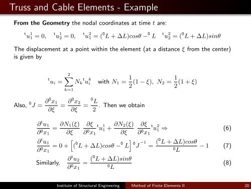
Truss <strong>and</strong> Cable <strong>Element</strong>s - Example<br />
From <strong>the</strong> Geometry <strong>the</strong> nodal coordinates at time t are:<br />
t u 1 1 = 0,<br />
t u 1 2 = 0,<br />
t u 2 1 = ( 0 L + ∆L)cosθ − 0 L<br />
t u 2 2 = ( 0 L + ∆L)sinθ<br />
<strong>The</strong> displacement at a point within <strong>the</strong> element (at a distance ξ from <strong>the</strong> center)<br />
is given by<br />
t u i =<br />
2∑<br />
k=1<br />
N t k u k i with N 1 = 1 2 (1 − ξ), N2 = 1 (1 + ξ)<br />
2<br />
Also, 0 J = ∂0 x 1<br />
∂ξ<br />
= ∂0 x 2<br />
∂ξ<br />
=<br />
0 L<br />
. <strong>The</strong>n we obtain<br />
2<br />
∂ t u 1<br />
= ∂N1(ξ)<br />
∂ 0 x 1 ∂ξ<br />
∂ t u 1<br />
∂ 0 x 1<br />
= 0 +<br />
Similarly,<br />
∂ξ t u 1<br />
∂ 0 1 + ∂N2(ξ)<br />
x 1 ∂ξ<br />
[<br />
( 0 L + ∆L)cosθ − 0 L<br />
∂ t u 2<br />
= (0 L + ∆L)sinθ<br />
∂ 0 x 0 1 L<br />
∂ξ t u 2<br />
∂ 0 1 ⇒ (6)<br />
x 1<br />
]<br />
0<br />
J −1 = (0 L + ∆L)cosθ<br />
− 1 (7)<br />
0<br />
L<br />
(8)<br />
Institute <strong>of</strong> Structural Engineering <strong>Method</strong> <strong>of</strong> <strong>Finite</strong> <strong>Element</strong>s II 20