Modeling Roaming in Large-scale Wireless Networks using Real ...

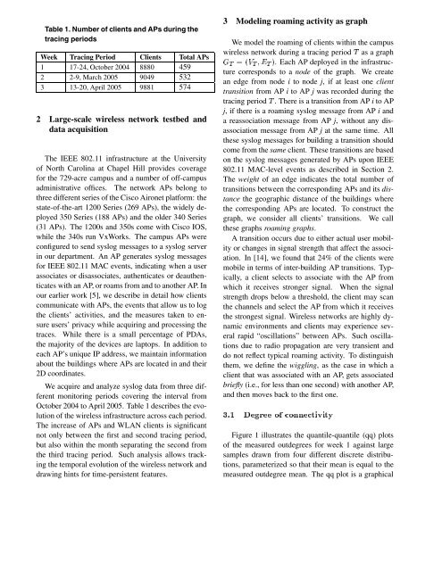
Table 1. Number of clients and APs during the
tracing periods
Week Tracing Period Clients Total APs
1 17-24, October 2004 8880 459
2 2-9, March 2005 9049 532
3 13-20, April 2005 9881 574
2 Large-scale wireless network testbed and
data acquisition
The IEEE 802.11 infrastructure at the University
of North Carolina at Chapel Hill provides coverage
for the 729-acre campus and a number of off-campus
administrative offices. The network APs belong to
three different series of the Cisco Aironet platform: the
state-of-the-art 1200 Series (269 APs), the widely deployed
350 Series (188 APs) and the older 340 Series
(31 APs). The 1200s and 350s come with Cisco IOS,
while the 340s run VxWorks. The campus APs were
configured to send syslog messages to a syslog server
in our department. An AP generates syslog messages
for IEEE 802.11 MAC events, indicating when a user
associates or disassociates, authenticates or deauthenticates
with an AP, or roams from and to another AP. In
our earlier work [5], we describe in detail how clients
communicate with APs, the events that allow us to log
the clients’ activities, and the measures taken to ensure
users’ privacy while acquiring and processing the
traces. While there is a small percentage of PDAs,
the majority of the devices are laptops. In addition to
each AP’s unique IP address, we maintain information
about the buildings where APs are located in and their
2D coordinates.
We acquire and analyze syslog data from three different
monitoring periods covering the interval from
October 2004 to April 2005. Table 1 describes the evolution
of the wireless infrastructure across each period.
The increase of APs and WLAN clients is significant
not only between the first and second tracing period,
but also within the month separating the second from
the third tracing period. Such analysis allows tracking
the temporal evolution of the wireless network and
drawing hints for time-persistent features.
3 Modeling roaming activity as graph
We model the roaming of clients within the campus
wireless network during a tracing period T as a graph
G T =(V T E T ). Each AP deployed in the infrastructure
corresponds to a node of the graph. We create
an edge from node i to node j, if at least one client
transition from AP i to AP j was recorded during the
tracing period T . There is a transition from AP i to AP
j, if there is a roaming syslog message from AP i and
a reassociation message from AP j, without any disassociation
message from AP j at the same time. All
these syslog messages for building a transition should
come from the same client. These transitions are based
on the syslog messages generated by APs upon IEEE
802.11 MAC-level events as described in Section 2.
The weight of an edge indicates the total number of
transitions between the corresponding APs and its distance
the geographic distance of the buildings where
the corresponding APs are located. To construct the
graph, we consider all clients’ transitions. We call
these graphs roaming graphs.
A transition occurs due to either actual user mobility
or changes in signal strength that affect the association.
In [14], we found that 24% of the clients were
mobile in terms of inter-building AP transitions. Typically,
a client selects to associate with the AP from
which it receives stronger signal. When the signal
strength drops below a threshold, the client may scan
the channels and select the AP from which it receives
the strongest signal. Wireless networks are highly dynamic
environments and clients may experience several
rapid “oscillations” between APs. Such oscillations
due to radio propagation are very transient and
do not reflect typical roaming activity. To distinguish
them, we define the wiggling, as the case in which a
client that was associated with an AP, gets associated
briefly (i.e., for less than one second) with another AP,
and then moves back to the first one.
3.1 Degree of connectivity
Figure 1 illustrates the quantile-quantile (qq) plots
of the measured outdegrees for week 1 against large
samples drawn from four different discrete distributions,
parameterized so that their mean is equal to the
measured outdegree mean. The qq plot is a graphical