Modeling Roaming in Large-scale Wireless Networks using Real ...

More documents

Recommendations

Info

Table 1. Number of clients and APs during the tracing periods Week Tracing Period Clients Total APs 1 17-24, October 2004 8880 459 2 2-9, March 2005 9049 532 3 13-20, April 2005 9881 574 2 Large-scale wireless network testbed and data acquisition The IEEE 802.11 infrastructure at the University of North Carolina at Chapel Hill provides coverage for the 729-acre campus and a number of off-campus administrative offices. The network APs belong to three different series of the Cisco Aironet platform: the state-of-the-art 1200 Series (269 APs), the widely deployed 350 Series (188 APs) and the older 340 Series (31 APs). The 1200s and 350s come with Cisco IOS, while the 340s run VxWorks. The campus APs were configured to send syslog messages to a syslog server in our department. An AP generates syslog messages for IEEE 802.11 MAC events, indicating when a user associates or disassociates, authenticates or deauthenticates with an AP, or roams from and to another AP. In our earlier work [5], we describe in detail how clients communicate with APs, the events that allow us to log the clients’ activities, and the measures taken to ensure users’ privacy while acquiring and processing the traces. While there is a small percentage of PDAs, the majority of the devices are laptops. In addition to each AP’s unique IP address, we maintain information about the buildings where APs are located in and their 2D coordinates. We acquire and analyze syslog data from three different monitoring periods covering the interval from October 2004 to April 2005. Table 1 describes the evolution of the wireless infrastructure across each period. The increase of APs and WLAN clients is significant not only between the first and second tracing period, but also within the month separating the second from the third tracing period. Such analysis allows tracking the temporal evolution of the wireless network and drawing hints for time-persistent features. 3 Modeling roaming activity as graph We model the roaming of clients within the campus wireless network during a tracing period T as a graph G T =(V T E T ). Each AP deployed in the infrastructure corresponds to a node of the graph. We create an edge from node i to node j, if at least one client transition from AP i to AP j was recorded during the tracing period T . There is a transition from AP i to AP j, if there is a roaming syslog message from AP i and a reassociation message from AP j, without any disassociation message from AP j at the same time. All these syslog messages for building a transition should come from the same client. These transitions are based on the syslog messages generated by APs upon IEEE 802.11 MAC-level events as described in Section 2. The weight of an edge indicates the total number of transitions between the corresponding APs and its distance the geographic distance of the buildings where the corresponding APs are located. To construct the graph, we consider all clients’ transitions. We call these graphs roaming graphs. A transition occurs due to either actual user mobility or changes in signal strength that affect the association. In [14], we found that 24% of the clients were mobile in terms of inter-building AP transitions. Typically, a client selects to associate with the AP from which it receives stronger signal. When the signal strength drops below a threshold, the client may scan the channels and select the AP from which it receives the strongest signal. Wireless networks are highly dynamic environments and clients may experience several rapid “oscillations” between APs. Such oscillations due to radio propagation are very transient and do not reflect typical roaming activity. To distinguish them, we define the wiggling, as the case in which a client that was associated with an AP, gets associated briefly (i.e., for less than one second) with another AP, and then moves back to the first one. 3.1 Degree of connectivity Figure 1 illustrates the quantile-quantile (qq) plots of the measured outdegrees for week 1 against large samples drawn from four different discrete distributions, parameterized so that their mean is equal to the measured outdegree mean. The qq plot is a graphical
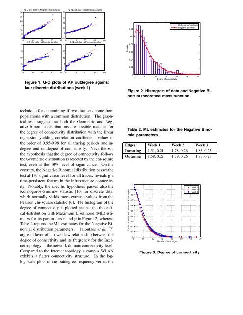
30 Q−Q plot data vs Neg Binomial samples 80 Q−Q plot data vs Geometric samples 25 60 20 40 15 20 10 5 0 0 −20 0 10 20 30 40 0 10 20 30 40 Q−Q plot data vs Binomial samples Q−Q plot data vs Poisson samples 20 20 15 15 Density 0.12 0.1 0.08 0.06 Histogram of real data Negative Binomial 10 10 0.04 5 0 0 10 20 30 40 5 0 0 10 20 30 40 Figure 1. Q-Q plots of AP outdegree against four discrete distributions (week 1) 0.02 0 0 5 10 15 20 25 30 Degree of connectivity Figure 2. Histogram of data and Negative Binomial theoretical mass function technique for determining if two data sets come from populations with a common distribution. The graphical tests suggest that both the Geometric and Negative Binomial distributions are possible matches for the degree of connectivity distribution with the linear regression yielding correlation coeffiecient values in the order of 0.95-0.98 for all tracing periods and indegree and outdegree of connectivity. Nevertheless, the hypothesis that the degree of connectivity follows the Geometric distribution is rejected by the chi-square test, even at the 10% level of significance. On the contrary, the Negative Binomial distribution passes the test at 1% significance level for all traces, revealing a time-persistent feature in the infrastructure connectivity. Notably, the specific hypothesis passes also the Kolmogorov-Smirnov statistic [16] for discrete data, which normally yields more extreme values from the Pearson chi-square statistic [6]. The histogram of the degree of connectivity is plotted against the theoretical distribution with Maximum Likelihood (ML) estimates for its parameters r and p in Figure 2, whereas Table 2 reports the ML estimates for the Negative Binomial distribution parameters. Faloutsos et al. [7] argue in favor of a power-law relationship between the degree of connectivity and its frequency for the Internet topology at the network domain connectivity level. Compared to the Internet topology, a campus WLAN exhibits a flatter connectivity structure. In the loglog scale plots of the outdegree frequency versus the Table 2. ML estimates for the Negative Binomial parameters Edges Week 1 Week 2 Week 3 Incoming 1.51, 0.21 1.78, 0.26 1.83, 0.25 Outgoing 1.58, 0.22 1.79, 0.26 1.73, 0.23 Fraction of nodes with more than x total edges 1 0.9 0.8 0.7 0.6 0.5 0.4 0.3 0.2 0.1 week 1 week 2 week 2 0 0 10 20 30 40 50 60 70 Number of total edges Figure 3. Degree of connectivity
Page 1: Modeling Roaming in Large-scale Wir
Page 5 and 6: Table 3. Evolution of crosspoints i

Modeling Roaming in Large-scale Wireless Networks using Real ...

Create successful ePaper yourself

Delete template?

Save as template?