Modeling Roaming in Large-scale Wireless Networks using Real ...

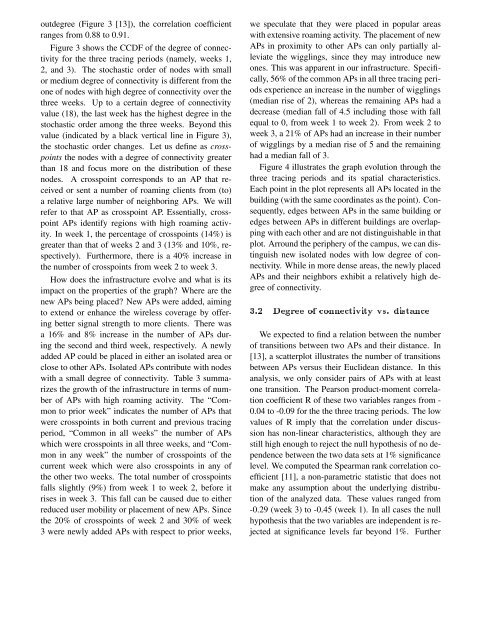
outdegree (Figure 3 [13]), the correlation coefficient
ranges from 0.88 to 0.91.
Figure 3 shows the CCDF of the degree of connectivity
for the three tracing periods (namely, weeks 1,
2, and 3). The stochastic order of nodes with small
or medium degree of connectivity is different from the
one of nodes with high degree of connectivity over the
three weeks. Up to a certain degree of connectivity
value (18), the last week has the highest degree in the
stochastic order among the three weeks. Beyond this
value (indicated by a black vertical line in Figure 3),
the stochastic order changes. Let us define as crosspoints
the nodes with a degree of connectivity greater
than 18 and focus more on the distribution of these
nodes. A crosspoint corresponds to an AP that received
or sent a number of roaming clients from (to)
a relative large number of neighboring APs. We will
refer to that AP as crosspoint AP. Essentially, crosspoint
APs identify regions with high roaming activity.
In week 1, the percentage of crosspoints (14%) is
greater than that of weeks 2 and 3 (13% and 10%, respectively).
Furthermore, there is a 40% increase in
the number of crosspoints from week 2 to week 3.
How does the infrastructure evolve and what is its
impact on the properties of the graph? Where are the
new APs being placed? New APs were added, aiming
to extend or enhance the wireless coverage by offering
better signal strength to more clients. There was
a 16% and 8% increase in the number of APs during
the second and third week, respectively. A newly
added AP could be placed in either an isolated area or
close to other APs. Isolated APs contribute with nodes
with a small degree of connectivity. Table 3 summarizes
the growth of the infrastructure in terms of number
of APs with high roaming activity. The “Common
to prior week” indicates the number of APs that
were crosspoints in both current and previous tracing
period, “Common in all weeks” the number of APs
which were crosspoints in all three weeks, and “Common
in any week” the number of crosspoints of the
current week which were also crosspoints in any of
the other two weeks. The total number of crosspoints
falls slightly (9%) from week 1 to week 2, before it
rises in week 3. This fall can be caused due to either
reduced user mobility or placement of new APs. Since
the 20% of crosspoints of week 2 and 30% of week
3 were newly added APs with respect to prior weeks,
we speculate that they were placed in popular areas
with extensive roaming activity. The placement of new
APs in proximity to other APs can only partially alleviate
the wigglings, since they may introduce new
ones. This was apparent in our infrastructure. Specifically,
56% of the common APs in all three tracing periods
experience an increase in the number of wigglings
(median rise of 2), whereas the remaining APs had a
decrease (median fall of 4.5 including those with fall
equal to 0, from week 1 to week 2). From week 2 to
week 3, a 21% of APs had an increase in their number
of wigglings by a median rise of 5 and the remaining
had a median fall of 3.
Figure 4 illustrates the graph evolution through the
three tracing periods and its spatial characteristics.
Each point in the plot represents all APs located in the
building (with the same coordinates as the point). Consequently,
edges between APs in the same building or
edges between APs in different buildings are overlapping
with each other and are not distinguishable in that
plot. Arround the periphery of the campus, we can distinguish
new isolated nodes with low degree of connectivity.
While in more dense areas, the newly placed
APs and their neighbors exhibit a relatively high degree
of connectivity.
3.2 Degree of connectivity vs. distance
We expected to find a relation between the number
of transitions between two APs and their distance. In
[13], a scatterplot illustrates the number of transitions
between APs versus their Euclidean distance. In this
analysis, we only consider pairs of APs with at least
one transition. The Pearson product-moment correlation
coefficient R of these two variables ranges from -
0.04 to -0.09 for the the three tracing periods. The low
values of R imply that the correlation under discussion
has non-linear characteristics, although they are
still high enough to reject the null hypothesis of no dependence
between the two data sets at 1% significance
level. We computed the Spearman rank correlation coefficient
[11], a non-parametric statistic that does not
make any assumption about the underlying distribution
of the analyzed data. These values ranged from
-0.29 (week 3) to -0.45 (week 1). In all cases the null
hypothesis that the two variables are independent is rejected
at significance levels far beyond 1%. Further