Instantaneous Point-source Solution - IfH

1 

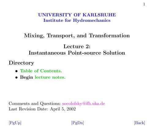
UNIVERSITY OF KARLSRUHE 

Institute for Hydromechanics 

Directory 

Mixing, Transport, and Transformation 

Lecture 2: 

Instantaneous Point-source Solution 

• Table of Contents. 

• Begin lecture notes. 

Comments and Questions: socolofsky@ifh.uka.de 

Last Revision Date: April 5, 2002 

[PgUp] [PgDn] [Back]

Table of Contents 2 

Instantaneous Point-source Solution 

Table of Contents 

1. Review of the advective diffusion equation 

1.1. Fickian diffusion 

1.2. Advection 

1.3. Advective-diffusion equation 

2. Moving coordinate system 

3. Similarity solution to the one-dimensional diffusion equation 

3.1. Dimensional analysis 

3.2. Coordinate transformation 

3.3. Solution 

4. Interpretation of the similarity solution 

5. Point-source solution with advection 

A. References 


Section 1: Review of the advective diffusion equation 3 

1. Review of the advective diffusion equation 

Diffusion has two primary properties: it is random in nature, and 

transport is from high concentration to low concentration regions, 

with an equilibrium state of uniform concentration. 

1.1. Fickian diffusion 

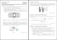
A static model of one-dimensional diffusion is given in Figure 1. This 

model can also be viewed as an animation. 

This motion is described by Fick’s law, given by 

( ∂C 

⃗q = −D 

∂x , ∂C 

∂y , ∂C ) 

∂z 

= −D∇C 

= −D ∂C . 

∂x i 

(1) 

Processes that obey this relationship are called Fickian diffusion processes. 

In water, D is of order 2·10 −9 m 2 /s (See Table 1). 



1.2. Advection 

In a current, the molecules experience two types of motion: 

• Due to diffusion, each molecule in time δt will move either one 

step to the left or one step to the right (i.e. ±δx). 

• Due to advection, each molecule will also move uδt in the crossflow 

direction. 

These processes are clearly additive and independent: we can use 

superposition. 

Thus, the advective-diffusive flux vector becomes 

⃗J = ⃗uC + ⃗q 

= u i C − D ∂C 

∂x i 

. (2) 



1.3. Advective-diffusion equation 

To derive the governing equation we use the control volume shown in 

Figure 2. From the conservation of mass, the net flux through the 

control volume is 

∂M 

∂t 

= ∑ J in − ∑ J out , (3) 

and for the x-direction, we have 

( 

∆J x = uC − D ∂C )∣ ( 

∣∣∣1 

δyδz − uC − D ∂C )∣ ∣∣∣2 

δyδz. (4) 

∂x 

∂x 

After using Taylor-series expansion we obtain 

∂C 

∂t + ∂(u iC) 

∂x i 

the governing Advective-Diffusion (A-D) equation. 

= D ∂2 C 

∂x 2 , (5) 

i 


Section 2: Moving coordinate system 6 

2. Moving coordinate system 

For one-dimensional diffusion in a steady flow, we can simplify (5) 

using a moving coordinate transformation. The new coordinates are 

ξ = x − (x 0 + ut) (6) 

τ = t, (7) 

The one-dimensional advective-diffusion equation with a steady current 

⃗u = (u, 0, 0) is 

∂C 

∂t + u∂C ∂x = D ∂2 C 

∂x 2 . (8) 

To perform the coordinate transformation, we must substitute the 

new coordinates into this equation. To do this we use the chain rule, 

giving 

∂C 

∂t 

∂C 

∂x 

= ∂C 

∂τ 

= ∂C 

∂τ 

∂τ 

∂t + ∂C ∂ξ 

∂ξ ∂t 

∂τ 

∂x + ∂C ∂ξ 

∂ξ ∂x 



From the definitions of the coordinate transformations we have 

and 

∂ξ 

∂t 

∂τ 

∂t 

= −u 

= 1 

∂ξ 

∂x = 1 

∂τ 

∂x = 0. 

Substituting into the governing equation (8) gives 

∂C ∂τ 

+ ∂C [ 

∂ξ ∂C 

∂τ ∂t ∂ξ ∂t + u ∂ξ 

∂ξ ∂x + ∂C ] 

∂τ 

= 

∂τ ∂x 

( ∂ ∂ξ 

D 

∂ξ ∂x + ∂ ) ( 

∂τ ∂C 

∂τ ∂x ∂ξ 

∂ξ 

∂x + ∂C 

∂τ 

) 

∂τ 

∂x 

(9) 



which reduces to 

∂C 

∂τ = D ∂2 C 

∂ξ 2 . (10) 

This is just the one-dimensional pure diffusion equation in the coordinates 

τ and ξ. 

Hence, we only need to find the point-source solution for pure 

diffusion. 


Section 3: Similarity solution to the one-dimensional diffusion equation 9 

3. Similarity solution to the one-dimensional diffusion 

equation 

Consider the one-dimensional inviscid problem of a narrow, infinite 

pipe (radius a) as depicted in Figure 3. A mass of tracer, M, is 

injected uniformly across the cross-section of area A = πa 2 at the 

point x = 0 at time t = 0. We seek a solution for the spread of tracer 

in time due to pure diffusion. 

The governing equation is 

∂C 

∂t = D ∂2 C 

∂x 2 (11) 

which requires two boundary conditions and an initial condition: 

• As boundary conditions, we impose that the concentration at 

±∞ remain zero: 

C(±∞, t) = 0. (12) 



• The initial condition is that the dye tracer is injected instantaneously 

and uniformly across the cross-section over an infinitesimally 

small width in the x-direction: 

C(x, 0) = (M/A)δ(x) (13) 

where δ(x) is zero everywhere accept at x = 0, where it is infinite, 

but the integral of the delta function from −∞ to ∞ is 1. 

Thus, the total injected mass is given by 

∫ 

M = C(x, t)dV (14) 

= 

V 

∫ ∞ ∫ a 

−∞ 

To find the solution we use the similarity method. 

0 

(M/A)δ(x)2πrdrdx. (15) 



3.1. Dimensional analysis 

To use dimensional analysis, we must consider all the parameters that 

control the solution. Table 4 summarizes the dependent and independent 

variables for our problem. There are m = 5 parameters and 

n = 3 dimensions; thus, we can form two dimensionless groups: 

π 1 = 

π 2 = 

C 

M/(A √ Dt) 

(16) 

x 

√ 

Dt 

(17) 

From dimensional analysis we have that π 1 = f(π 2 ), which implies 

for the solution of C: 

C = 

M ( ) x 

A √ Dt f √ (18) 

Dt 

where f is a yet-unknown function with arguement π 2 . (18) is called 

a similarity solution because C has the same shape in x at all times t. 



3.2. Coordinate transformation 

The similarity solution represented by (18) is really just a coordinate 

transformation. The new coordinate η = x/ √ Dt is called the 

similarity variable. For the coordinate transformation we have: 

Thus, we must 

η = 

1. Substitute C = M/(A √ Dt)f(x/ √ Dt). 

2. Substitute η = x/ √ Dt. 

x 

√ 

Dt 

(19) 

∂η 

= − η (20) 

∂t 2t 

∂η 

∂x = 1 

√ . (21) 

Dt 



Using the chain rule to compute ∂C/∂t we have: 

∂C 

= ∂ [ ] M 

∂t ∂t A √ Dt f(η) ( 

M 

= 

A √ − 1 ) 1 

Dt 2 t f(η) + M 

A √ Dt 

= − M ( 

2At √ f + η ∂f 

Dt ∂η 

∂f ∂η 

∂η ∂t 

Using the chain rule to compute ∂ 2 C/∂x 2 we have: 

∂ 2 C 

∂x 2 = ∂ [ ( ∂ M 

∂x ∂x 

= ∂ 

∂x 

= 

[ ∂η 

∂x 

M 

ADt √ Dt 

∂f 

∂η 

) 

. (22) 

A √ Dt f(η) )] 

M 

] 

A √ Dt 

∂ 2 f 

∂η 2 . (23) 



After substituting these two results into the diffusion equation, we 

obtain the ordinary differential equation in η 

d 2 f 

dη 2 + 1 ( 

f + η df ) 

= 0. (24) 

2 dη 

3.3. Solution 

To solve (24) we first make use of the identity 

d(fη) 

dη 

= f + η df 

dη . (25) 

Substituting gives us 

[ 

d df 

dη dη + 1 ] 

2 fη = 0. (26) 

To solve this equation requires two integrations. 



1. Integrating once leaves us with 

df 

dη + 1 2 fη = C 0. (27) 

It can be shown that choosing C 0 = 0 satisfies both boundary 

conditions and the initial condition (see Appendix B in the class 

notes). 

2. The second integration requires a little algebra. First, move the 

second term to the right-hand-side. 

df 

dη = −1 fη. (28) 

2 

Next, like terms: 

df 

f = −1 ηdη. (29) 

2 

Finally, integrate both sides: 

) 

f = C 1 exp 

(− η2 

. (30) 

4 



To find C 1 we must use the conservation of mass: 

∫ 

M = C(x, t)dV 

= 

= M 

which gives the constraint 

∫ ∞ 

−∞ 

V 

∫ ∞ ∫ a 

−∞ 0 

∫ ∞ 

−∞ 

C(η)2πrdr √ Dtdη 

f(η)dη 

( 

C 1 exp − η ) 

dη = 1. (31) 

4 

To solve this integral we need to make one more change of variables 

to remove the 1/4 from the exponential. Thus, we introduce ζ such 

that 

ζ 2 = 1 4 η2 (32) 

2dζ = dη. (33) 



Solving for C 1 leaves 

1 

C 1 = 

2 ∫ ∞ 

−∞ exp(−ζ2 )dζ , (34) 

and after looking up the integral in a table, we obtain C 1 = 1/(2 √ π). 

Thus, f = exp(η 2 /4)/(2 √ π), and our similarity solution is 

( ) 

M 

C(x, t) = 

A √ 4πDt exp − x2 

. (35) 

4Dt 


Section 4: Interpretation of the similarity solution 18 

4. Interpretation of the similarity solution 

Figure 4 shows the solution (35) in non-dimensional space. The 

animation also plots this solution, confirming that our solution is valid 

for a Fickian diffusion process. 

Comparing (35) with the Gaussian probability distribution reveals 

that (35) is the normal bell-shaped curve with a standard deviation, 

σ, of width 

σ 2 = 2Dt. (36) 

The concept of self similarity is now also evident: the concentration 

profile shape is always Gaussian. By plotting in non-dimensional 

space, the profiles also collapse into a single profile; thus, profiles for 

all times t > 0 are given by the result in the figure. 


Section 5: Point-source solution with advection 19 

5. Point-source solution with advection 

The final step is to substitute the coordinate transformation for the 

moving reference frame into the point source solution (35). In the 

moving coordinate system, this solution is 

( ) 

M 

C(ξ, τ) = 

A √ 4πDτ exp − ξ2 

. (37) 

4Dτ 

Our coordinate transformation was ξ = x − (x 0 + ut) and τ = t. 

Substituting into (37) gives: 

( 

M 

C(x, t) = 

A √ 4πDt exp − (x − (x 0 + ut) 2 ) 

. (38) 

4Dt 

Figure 5 shows the schematic behavior of this solution for three different 

times, t 1 , t 2 , and t 3 . A second animation shows this solution 

in action. 


Figures and tables 20 

Figure 1: Schematic of the one-dimensional molecular (Brownian) motion 

of a group of molecules illustrating the Fickian diffusion model. 

The upper part of the figure shows the particles themselves; the lower 

part of the figure gives the corresponding histogram of particle location, 

which is analogous to concentration. 

(a.) Initial 

distribution 

(b.) Random 

motions 

(c.) Final 

distribution 

n 

n 

n 

0 x 

0 x 

0 

x 



Table 1: Molecular diffusion coefficients for typical solutes in water 

at standard pressure and temperature (20 ◦ C). a 

Solute name Chemical symbol Diffusion coefficient b 

hydrogen ion H + 0.85 

hydroxide ion OH − 0.48 

oxygen O 2 0.20 

carbon dioxide CO 2 0.17 

bicarbonate HCO − 3 0.11 

carbonate 

CO 2− 

3 0.08 

methane CH 4 0.16 

ammonium NH + 4 0.18 

ammonia NH 3 0.20 

(10 −4 cm 2 /s) 



Table 2: Molecular diffusion coefficients (continued). 


nitrate NO − 3 0.17 

phosphoric acid H 3PO 4 0.08 

dihydrogen phosphate H 2PO − 4 0.08 

hydrogen phosphate 

phosphate 

HPO 2− 

4 0.07 

PO 3− 

4 0.05 

hydrogen sulfide H 2S 0.17 

hydrogen sulfide ion HS − 0.16 

sulfate 

SO 2− 

4 0.10 

silica H 4SiO 4 0.10 

(10 −4 cm 2 /s) 



Table 3: Molecular diffusion coefficients (continued). 


calcium ion Ca 2+ 0.07 

magnesium ion Mg 2+ 0.06 

iron ion Fe 2+ 0.06 

manganese ion Mn 2+ 0.06 

a Taken from diffusion coefficients web page 

b for water at 20 ◦ C with salinity of 0.5 ppt. 

c for water at 10 ◦ C with salinity of 0.5 ppt. 

(10 −4 cm 2 /s) 



Figure 2: Schematic of a control volume with crossflow. 

z 

J x,in 

δz 

J x,out 

x 

u 

-y 

δx 

δy 



Figure 3: Definitions sketch for one-dimensional pure diffusion in an 

infinite pipe. 

-x x 

A 

M 



Table 4: Dimensional variables for one-dimensional pipe diffusion. 

Variable 

Dimensions 

dependent variable C M/L 3 

independent variables M/A M/L 2 

D L 2 /T 

x 

L 

t 

T 



Figure 4: Self-similarity solution for one-dimensional diffusion of an 

instantaneous point source in an infinite domain. 

1 

Point source solution 

C A (4πD t) 1/2 / M 

0.8 

0.6 

0.4 

0.2 

0 

−4 −2 0 2 4 

η = x / (4Dt) 1/2 



Figure 5: Schematic solution of the advective-diffusion equation in 

one dimension. The dotted line plots the maximum concentration as 

the cloud moves downstream. 

1.5 

Solution of the advective−diffusion equation 

C max 

Concentration 

1 

0.5 

t 1 

t 2 t3 

0 

0 1 2 3 4 5 6 7 8 9 10 

Position 


References 

Fischer, H. B., List, E. G., Koh, R. C. Y., Imberger, J. & Brooks, 

N. H. (1979), Mixing in Inland and Coastal Waters, Academic 

Press, New York, NY.

Instantaneous Point-source Solution - IfH

You also want an ePaper? Increase the reach of your titles

Delete template?

Save as template?