user's manual for corhyd: an internal diffuser hydraulics model - IfH

Universität Karlsruhe
Institut für Hydromechanik
Kaiserstr. 12
D-76128 Karlsruhe
Tel.: +49 (0)721/608-2200, -2202
Fax: +49 (0)721/66 16 86
ifh@uni-karlsruhe.de
www.ifh.uni-karlsruhe.de
Bericht Nr. xxx
USER'S MANUAL FOR CORHYD:
AN INTERNAL DIFFUSER
HYDRAULICS MODEL
Bearbeiter:
Dipl.-Ing. T. Bleninger
Karlsruhe, June 2005

Version 1.0, June 2005
USER'S MANUAL FOR CORHYD:
AN INTERNAL DIFFUSER HYDRAULICS MODEL
by
Tobias Bleninger, Gerhard H. Jirka
Institute for Hydromechanics, University Karlsruhe
Kaiserstr. 12, 76128 Karlsruhe, Germany, bleninger@ifh.uka.de
http://www.cormix.de/corhyd.htm
Abstract
Submerged multiport diffusers for waste water outfalls are designed often, considering steady
flow conditions for far future scenarios. Design aims for lower costs for material use and
pumping energy and the minimization of environmental impacts. Inadequate attention on the
internal diffuser hydraulics also for off design conditions thereby often result in hydraulic
problems like partial blockage, high head losses, uneven flow distribution, salt water intrusion
and poor dilution causing higher energy demands and stronger environmental impacts.
The CorHyd computer program has been developed for the calculation of velocities,
pressures, head losses and flow rates inside the diffuser pipe and, especially, at the diffuser
port orifices to analyze and optimize diffuser design alternatives as well as existing diffuser
configurations for different and varying discharge and ambient conditions. The calculation is
based on the application of the steady continuity and work-energy equations between ambient
fluid at the discharge points and the effluent inside the diffuser pipe. Emphasis was given to
the implementation of all occurring losses especially if high risers, duckbill valves, multiple
ports and more complex discharge configurations are applied.
Detailed calculations for the internal manifold hydraulics in the outfall pipes show a strong
sensitivity on the representation and formulation of local losses even for relatively simple
riser/port configurations. An optimization methodology yields a homogeneous discharge
distribution along the diffuser, minimization of the total head and prevention of sedimentation
or ambient water intrusion in the diffuser under varying inflow and ambient conditions. The
final design achieves lower costs for material use and operation as well as the minimization of
environmental impacts and operational stability for off-design conditions.
i

Acknowledgments
The authors like to express their gratitude to the student assistants Martina Kurzke and Jan
Müller who contributed to the coding of the present program. Thanks to Rob Doneker from
Mixzon Inc. for his friendly and scientific help and the offer to include the program in
CORMIX, the Cornell Mixing Zone Expert System. We furthermore appreciated the data
support from TideFlex Technologies from RedValve Company and Elasto-Valve Rubber
Products (EVR) company for developing loss formulations for duckbill valves.
Institut für Hydromechanik, Universität Karlsruhe
ii

Contents
Abstract ....................................................................................................................................... i
Acknowledgments......................................................................................................................ii
Contents...................................................................................................................................... 1
Glossary...................................................................................................................................... 3
1 Introduction ........................................................................................................................ 4
1.1 Installation and start ................................................................................................... 4
2 Background ........................................................................................................................ 5
2.1 Multiport diffusers...................................................................................................... 5
2.2 External hydraulics - dilution requirements............................................................... 7
2.3 Internal hydraulics - operational requirements........................................................... 8
2.4 Manifold processes................................................................................................... 10
2.4.1 Local loss formulations .................................................................................... 12
2.4.2 Friction losses................................................................................................... 19
3 General Features of CorHyd ............................................................................................ 23
3.1 Major Assumptions .................................................................................................. 23
3.1.1 Steady flow....................................................................................................... 23
3.1.2 Single phase pressure pipe ............................................................................... 27
3.1.3 Geometrical assumptions ................................................................................. 27
3.1.4 Automatic implementation of loss formulations - additional losses................ 28
3.2 Governing Equations................................................................................................ 28
3.3 Solving scheme ........................................................................................................ 31
3.3.1 Solving for total head ....................................................................................... 31
3.3.2 Solving for total flow ....................................................................................... 31
3.4 System processing sequence and structure of simulation elements ......................... 33
4 Data Input......................................................................................................................... 36
4.1 Ambient Data ........................................................................................................... 37
4.2 Effluent Data ............................................................................................................ 38
4.3 Feeder and diffuser................................................................................................... 38
4.4 Port / Riser configurations........................................................................................ 39
4.5 Additional local losses (sub-menu).......................................................................... 40
4.6 Blocked ports (sub-menu) ........................................................................................ 41
4.7 Y or T-diffuser (sub-menus) .................................................................................... 41
5 Data Output ...................................................................................................................... 43
5.1 Report....................................................................................................................... 43
5.2 Graphical output....................................................................................................... 44
6 Design and optimization................................................................................................... 46
6.1 Far future design conditions..................................................................................... 47
6.2 Boundary condition variations ................................................................................. 48
6.3 Off design conditions ............................................................................................... 50
6.4 Sensitivity Analysis.................................................................................................. 50
7 Case studies...................................................................................................................... 52
7.1 Ipanema - Rio de Janeiro - Brazil............................................................................. 52
7.1.1 Diffuser optimization ....................................................................................... 58
7.2 Berazategui - Buenos Aires - Argentina .................................................................. 68
8 Conclusions ...................................................................................................................... 72
9 References ........................................................................................................................ 72
10 Annex ........................................................................................................................... 76
Institut für Hydromechanik, Universität Karlsruhe 1

10.1 Local loss formulations: Division of flow (Idelchik)............................................... 76
10.2 Local loss formulations: Orifices (Idelchik) ............................................................ 79
Institut für Hydromechanik, Universität Karlsruhe 2

Glossary
Table 1: Summary of parameters, Parameters are used with the following major indices: d = diffuser
pipeline section; p = port pipe; j = jet
Parameter Dimension Definition
ρ a kg/m³ average density of ambient water body
ρ e kg/m³ average density of the effluent
A m² pipe cross sectional area
B m equivalent slot width B = A p /l
C c - jet contraction coefficient
D m internal pipe diameter
E m energy head
g’ m/s² reduced gravity, g’ = ∆ρ/ρg
H m head above datum (additional indices: H t = total head at headworks; H d = design
water level elevation of ambient water)
i - numbering of port/riser configurations (counting from seaward end to shore,
starting with 1)
j - numbering of local losses in ports, risers or the diffuser
j 0 m³/s³ buoyancy flux per diffuser length, j 0 =g’q 0
k s m equivalent sand roughness
l m riser spacing
L m length of the considered pipe section
n - total number of local losses j in between one pipe section
N - total number of port/riser locations i of diffuser
N d - total number of diffuser sections (includes feeder)
N g - total number of port/riser groups
N gp - number of risers per group
N p - number of ports per riser
p Pa = N/m² pressure, (additional indices: p l = pressure loss, p a = ambient water pressure)
Q m³/s total flow through outfall system
q m³/s individual discharge through a riser or port at position i
q 0 m²/s mass flux per diffuser length , q 0 = V j B
R m radius of bend
Re - Reynolds number Re = VD/ν
S c - plume centerline dilution
SecNo - diffuser segment number where this group is located in
t s time
V m/s mean flow velocity
x m horizontal coordinate of pipe segment centerline location
y m horizontal coordinate of pipe segment centerline location
z m position or elevation in the vertical
α i - 1 / (number of ports at a riser at position i)
β ° angle of gradual expansion or contraction
ζ - dimensionless loss coefficient for local losses
λ - dimensionless friction coefficient
ν m²/s kinematic viscosity
Institut für Hydromechanik, Universität Karlsruhe 3

1 Introduction
CorHyd is a computer code for the calculation of flow characteristics in multiport diffuser
constructions. It includes loss calculations for complex geometries, as well as additional flow
forcing due to density differences.
CorHyd is a code written within the commercial software MatLab Release 14 from the
company Mathworks. The code includes a graphical user interface and allows to use all
MatLab functions for graphics, analysis and also further modifications. CorHyd is no selfexecutable
and needs MatLab to be installed. But also open source softwares like Scilab
(http://scilabsoft.inria.fr/) or Octave (http://www.octave.org) allow to import and execute the
MatLab based CorHyd files. CorHyd is an open source code and allows for easy
modifications. Downloads of the code and this manual, as well as further information are
available under: http://www.cormix.de/corhyd.htm.
An additional version is foreseen to be included into CORMIX (Cornell Mixing Zone Expert
System from MixZon, www.cormix.info). It is based on the same algorithm and includes the
same loss formulations, but uses the CORMIX interface and allows for easy data transfer
between an external hydraulics calculation with CORMIX and the internal hydraulics
calculation with CorHyd.
Publications from Bleninger et.al, 2002 and Bleninger et.al, 2005 describe scientific basis and
demonstrate comparisons and validation.
The objectives of this manual are: a) to provide comprehensive description of CorHyd, b)
give guidance for assembly and preparation of required input data, c) delineate ranges of
applicability, d) guidance for interpretation of results, and e) to illustrate practical application.
1.1 Installation and start
Unzip the matlab files into one folder on your computer. Run Matlab and change to the folder,
where the files have been saved as your working directory. Type IDH and the graphical user
interface opens up. Open an existing test file and press run to do the first calculation.
Institut für Hydromechanik, Universität Karlsruhe 4

2 Background
2.1 Multiport diffusers
Waste water treatment plants commonly discharge treated effluents through outfalls into
rivers or coastal waters. These plants are designed to minimize environmental impacts by
reducing the pollutant concentrations of the effluent. Nevertheless, even discharges of stateof-the-art
treatment plants may cause local pollution of the receiving waters, if the effluent
contains persistent substances and especially if discharge flowrates are high, which is the case
for most large metropolitan areas (like Buenos Aires, New York, Rio de Janeiro, HongKong,
Boston, Istanbul, …). To prevent local pollution and to protect ecologically sensitive regions,
persistent substances have to be reduced directly at the source and the large discharges have to
be distributed over a wider area. For the latter purpose, long outfall pipes with multiport
diffuser installations are used to disperse the effluent to non-critical levels (Jirka and Lee,
1994), aided by the natural pollution degradation rates of the receiving water bodies.
An optimized combination of on-land treatment and receiving water capacities, especially for
nutrient inputs from municipal sources, may positively affect the world’s severe health
problems often directly caused by sanitation problems (UNEP, 2004). New water quality
regulations (e.g., US: EPA, 1994; Europe: EC-Water framework directive, 2000; Brazil:
CONAMA, 2000; Argentina / Uruguay: Guarga et al. 1992) account for that combined
approach and therefore also result in a worldwide increasing utilization of treatment plants
with multiport diffuser outfalls (e.g., Australia: Philip and Pritchard, 1996; USA: Signell et
al., 2000).
An outfall is a pipe system between the dry land and the receiving water. It consists of three
components (Fig. 1): the onshore headwork (e.g. gravity or pumping basin); the feeder
pipeline which conveys the effluent to the disposal area; and the diffuser section, where a set
of ports releases and disperses the effluent into the environment to minimize the impacts on
the quality of the receiving water body. Diffusers can be single branched or double branched
systems (T- or Y-shaped, Fig. 2). If the the diffuser section is simply laid on the sea bed it is
composed of port orifices in the wall of the diffuser pipe (simple port configuration, Fig. 3a),
which may carry additional elements like elastic, variable area orifices (duckbill valves, Fig.
3b). If diffusers are covered with ballast, laid in a trench or even tunneled in the ocean floor
vertical risers (riser/port configuration, Fig. 3c) are connected to the diffuser to convey the
effluent to the water body. For deep tunneled solutions often rosette-like port arrangements
(similar to a gas burner device, Fig. 3d) are used to save the number of risers and allow for
increased dispersion. Also risers may carry duckbill valves, which change their effective open
port area related to the pressure difference between inside and outside the valve. They avoid
salt water intrusion during low flow periods and allow high discharges during peak flow
periods.
The flow in multiport diffusers is controlled by two boundary conditions: first, the entrance
boundary (flow rate or head), and, second, the ambient/disposal boundary, where the effluent
physical properties differ from the ambient fluid. Both conditions vary in time due to
discharge variations (diurnal changes, storm water events and long-term changes due to
increased sanitation coverage) and pressure variations, density variations, tides or waves.
Institut für Hydromechanik, Universität Karlsruhe 5

Fig. 1: Outfall configuration showing feeder pipe and diffuser from side view and top view, defining
the pipelines and port/riser configurations
Fig. 2: Left: standard diffuser, Right: Y- or T-shape diffuser configuration
Institut für Hydromechanik, Universität Karlsruhe 6

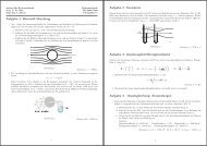
Fig. 3: a) simple port (source: Carlo Avanzini), b) Variable-area orifices (‘duckbill valves’, Image:
RedValve Company), c) riser/port configuration (Guarajá outfall, Sao Paulo State, Brazil), d)
rosette like port arrangement (Boston Outfall, Image: Massachusetts Water Resources
Authority, Boston, USA)
Typical outfalls are several kilometers long and discharge up to 1 m³/s treated effluent
through a few ten up to a hundred m long diffuser section with 10 - 50 ports in 10 to 40
meters depth. These constructions may cost a few million Euro (Gunnerson, 1988) and are
difficult to construct and maintain due to deep sea diving limits, the strong dependency on
weather conditions and the need for uninterrupted discharge for operating systems. Therefore
savings in construction and operation are of major importance.
An outfall design must consider both, the hydraulics occurring outside and inside a diffuser.
External hydraulics affect the effluent mixing with the ambient fluid, internal hydraulics
affect the flow partitioning and related pressure losses in the manifold resulting in a discharge
profile along the diffuser. CorHyd covers the internal diffuser hydraulics.
2.2 External hydraulics - dilution requirements
First design steps for the external hydraulics of diffusers are either the usage of simple
dilution equations (e.g. Jirka, 2003 or Jirka and Lee 1994) or the direct application of more
detailed mixing models (e.g. CORMIX) under given dilution requirements and major choices
for the riser/port spacing to find a minimum diffuser length and a first port diameter estimate.
All external hydraulic design methodologies and programs (mixing calculations) are based on
properly working diffusers and therefore use homogeneous discharge distributions along the
diffuser line as input. Effects of a non-homogeneous discharge distribution can be estimated
by simple (conservative) dilution equations for multiport diffusers (Jirka and Lee, 1996), valid
for the assumption of a 2-D plume after single jet merging (see Fig. 4). The plume centerline
dilution S c for stagnant water can be obtained with
S c = 0.38⎜ ⎛ j 1/3 0 z
⎝ q ⎠ ⎟⎞
(1)
0
Institut für Hydromechanik, Universität Karlsruhe 7

where j 0 denotes the buoyancy flux per diffuser length j 0 =g’q 0 , with g’= ∆ρ e
ρ a
g and q 0 = V j B,
the mass flux per diffuser length with the port exit velocity V j and the equivalent slot width
B = A p /l (A p is the port cross section and l the riser spacing, see Fig. 4). z is the observed
position in the vertical above the discharging port.
2-D
z
z
Merging level
2-D Zone
3-D
l
a 0
Fig. 4: Definition diagram for plume centerline dilution equation for multiport diffusers
A simple estimate of effects from a distorted discharge profile is a comparison of the
centerline dilution for two different mass fluxes:
S c1
S
= j 0,1 1/3 q 0,2
1/3
c2 q 0,1 j
= q 0,1 1/3 q 0,2
1/3
0,2 q 0,1 q
= ⎜ ⎛
0,2 ⎝
2/3
q 0,2
q 0,1
⎠ ⎟⎞
(2)
A 10% discharge variation q 0,2 /q 0,1 = 0.9 along a diffuser would therefore, result in dilution
difference of 7% (S c1 /S c2 = 0,93) along the diffuser line. These differences are often not
considered in further mixing calculations and so far could harm the environment or could lead
to critical concentrations with respect to the discharge permit.
The combination of CorHyd with CORMIX allows to find an optimized internal hydraulics
design (cost effective) resulting in environmental sound solutions.
2.3 Internal hydraulics - operational requirements
CorHyd covers the internal diffuser hydraulics with the following design objectives:
• uniform discharge distribution along the diffuser in order to meet dilution requirements
and to prevent operational problems (e.g. intrusion of ambient water through ports with
low flow). Exceptions should avoid near-shore impacts by keeping the seaward discharge
higher.
• minimized constructional and operational costs using simple manifold geometries with
small losses
• prevention of off-design operational problems in order to avoid particle deposition and
salt water intrusion during low flow or no-flow periods
Institut für Hydromechanik, Universität Karlsruhe 8

• performance tests against unsteady operations in order to reach rapidly steady flow
condition after purging during start-up, optimize intermittent pumping cycles and
consider wave induced circulations and water-hammer
Conflicting design parameters require compromises, which are often not sufficiently resolved
(Bleninger et. al, 2004). Existing diffuser programs (Fischer et al., 1979, implemented as code
PLUMEHYD; and Wood et al., 1993, implemented as DIFF) have deficiencies for diffuser
designs other than pipes with simple ports in the wall. They only consider short risers with
negligible friction losses and local losses and lack the implementation of long risers (like in
deep-tunneled outfalls) with meaningful frictional and local losses, Y-shaped diffusers,
complex port/riser configurations, multiple ports on one riser, duckbill valves or other
complex port losses. Design rules regarding the velocity ratios (Fischer et al., 1979) or loss
ratios (Weitbrecht et al., 2002) for diffuser sections and downstream ports are only helpful for
simple geometries (no changes along the diffuser). For others, they are either unnecessarily
conservative or not valid at all, because velocities and losses are changing drastically in actual
diffuser installations. Moreover these problems are often not recognized due to poor
monitoring conditions in deep sea. Consequences are costly systems in terms of construction,
operation and maintenance as well as bad dilution characteristics (Fig. 5).
Fig. 5: Replaced diffuser, which was full of sediment and therefore not working properly (courtesy of
Eng. Pedro Campos, Chile)
CorHyd calculates velocities, pressures, head losses and flow rates inside the diffuser pipe
and especially at the diffuser port orifices. Planner, designer and operator of outfalls may use
it to analyze, predict and monitor the discharge behavior of planned or installed diffusers
under different boundary conditions. The combination with CORMIX will provide a direct
linkage to subsequent waste plume modeling and mixing zone analysis.
Institut für Hydromechanik, Universität Karlsruhe 9

2.4 Manifold processes
Pipe hydraulics are characterized by continuous pressure losses due to wall friction and by
local pressure losses due to geometrical changes. Manifold hydraulics (i.e. diffusers) are
characterized by several flow separations, where local losses depend not only on geometrical
relations but furthermore on the discharge rates. The flow distribution for simple pipe
configurations with uniform geometries along the diffuser depends mainly on the ratio of
branching losses and manifold losses. But most of the actual diffuser geometries have more
complex geometries. Diffusers often discharge fluids with higher or lower density than the
receiving waters, which cause an additional buoyant forcing on the fluid flow.
Implemented losses in CorHyd include continuous losses due to friction in all pipes (feeder,
diffuser, riser, and port). Local losses are considered automatically in all pipe sections, the
feeder pipe, the diffuser manifold and the attached port-riser branches. Furthermore additional
local losses may be added manually if necessary:
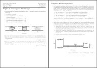
Local Feeder losses (Fig. 6)
• inlet loss at headworks
• horizontal and vertical bends
• contractions/expansions along the feeder pipe
• flow separation, if several diffusers are mounted on one feeder
Fig. 6: Local feeder losses
Diffuser manifold losses (Fig. 7)
Implemented local losses along a streamline along the diffuser pipe centerline passing the
branch pipes are:
• the division of flow loss for the diffuser pipe passing a riser
• horizontal or vertical bends
• contractions/expansions along the diffuser pipe
Institut für Hydromechanik, Universität Karlsruhe 10

Fig. 7: Local diffuser manifold losses
Port - riser branch losses
Implemented local losses along a streamline going from a diffuser centerline into the riser,
then into the port and the discharging jet are:
• the division of flow from the diffuser pipe into a riser
• optional: bends or additional losses in the riser
• the transition or division of flow from riser to port(s)
• optional: additional losses in the port or at the orifice
• optional: contraction of jet
• optional: duckbill valves at the port orifices
Optional means, that either additional known geometry changes or local loss coefficients can
manually be added to the generally foreseen local losses in ports and risers. If for example the
port is mounted perpendicular onto the riser, this local bending loss is not included but can be
added as a known loss. If a riser has more than one port, it is assumed, that the discharge
flowing through the riser, is distributed evenly among all ports (i.e. for two ports, both would
have half the discharge).
Institut für Hydromechanik, Universität Karlsruhe 11

Fig. 8: Local port/riser branch losses
2.4.1 Local loss formulations
Local losses are due to geometrical differences between one cross-sectional area of a pipe and
the adjacent one (i.e. expansions, contractions, or bends, Fig. 9) or the inlet or end of a pipe
(orifice). These changes may lead to flow detachment processes, reverse currents in
deadzones, locally increased accelerations or decelerations, increased turbulence, which all
cause energy losses, in closed pipe systems compensated by pressure losses.
Local pressure losses p l in a pipe system are generally calculated as:
p l =
ρ ⋅ V 2
e
V 2
ζ ⋅ or as headloss p l /γ e = ζ ⋅
(3)
2
2g
where ζ denotes the dimensionless loss coefficient, ρ e the effluent density and V the reference
velocity either upstream or downstream the geometrical change.
There are numerous publications defining local loss coefficients ζ for a large number of
different geometries under different flow conditions. Thus ζ itself may depend on the
Reynolds number, the actual flow condition (e.g. flowrate ratios in diverging flows) the
distance to previous local losses and geometrical reltions. Comparisons between these
publications showed discrepancies even for simple geometries. The choice was in regards to
the most accurate works from Idelchik (1986), Miller (1990), and Lee et.al. (1998).
Table 2 gives an overview of implemented local loss coefficients ζ. They are calculated
automatically in CorHyd. These assume reasonable high Reynolds numbers (above 10 4 ) and
reasonable geometrical distance between the changes to avoid interaction of losses.
Modification of the listed formulations can be found in Idelchik (1986) for special geometries
and some limited ranges of Reynolds numbers, although those are not implemented in
CorHyd. Furthermore additional optional losses can be added manually for risers and ports.
Examples for non-conventional nozzles or flanged orifices are given in the Annex, chapter 10.
Institut für Hydromechanik, Universität Karlsruhe 12

Fig. 9: Examples for local losses in pipe flows (Miller, 1990)
Institut für Hydromechanik, Universität Karlsruhe 13

Table 2: Local loss formulations
Type of
Loss
Inlet
(Reference
velocity is
V)
Definition
Sharp edged inlet (Idelchik, 1986)
ζ = 0.5
Code (see files: barchart.m, plotlosses.m, report.m, time_series.m, totalHead.m):
The value ζ = 0.5 is automatically foreseen in the code, if a feeder pipe exists. The loss is added
only after the whole calculation directly in the result files. Although most of the constructions do
have sharp edged inlets from the headworks into the feeder pipe other configurations may applied
by using the following graphs and changing the code in the mentioned files (zeta_entry = “new
value”).
Rounded inlets (Idelchik, 1986, Miller, 1978)
Institut für Hydromechanik, Universität Karlsruhe 14

Expansion
(Reference
velocity is
V 1 )
Sudden expansion (Idelchik, 1986)
ζ
e
⎛ A =
⎜1
−
⎝ A
1
2
⎞
⎟
⎠
2
Code (see files: CommonFeederPipe.m, feederpipes.m, DiffuserLosses.m,
Losses_common_feeder.m).
Gradual expansion (Idelchik 1986)
β
ζ
e
= 3.2 ⋅ tan ⋅
2
with β in rad
4
A1
tan
β ⎞
1
2
⎜
⎛ − A
⎟
⎝ 2 ⎠
2
For β > 50°, the formulation for gradual expansion leads to a greater loss coefficient than the one
for a sudden expansion. Therefore Idelchiks formulas was adopted so that for β > 50° losses are
equal the loss for β = 50°.
Code (see files: CommonFeederPipe.m, feederpipes.m, DiffuserLosses.m,
Losses_common_feeder.m).
Contraction
(Reference
velocity is
V 2 )
Sudden contraction (Idelchik, 1986)
⎛ A ⎞
ζ
2
c = 0.5 ⋅
⎜1
−
A
⎟
⎝ 1 ⎠
3 / 4
Code (see files: CommonFeederPipe.m, feederpipes.m, DiffuserLosses.m,
Losses_common_feeder.m).
Institut für Hydromechanik, Universität Karlsruhe 15

Gradual contraction (Idelchik 1986)
4
3
2
( − .0125⋅
n + 0.0224⋅
n − 0.00723⋅
n + 0.0044⋅
n − 0.00745)
3 2
ζ
c
= 0
0
0
0
0
⋅ ( β − 2πβ
−10β)
with A0
and β in rad
n = 1.0 A
0
≤
1
For β > 50°, the formulation for gradual expansion leads to a greater loss coefficient than the one
for a sudden expansion. Therefore Idelchiks formulas was adopted so that for β > 50° losses are
equal the loss for β = 50°.
Code (see files: CommonFeederPipe.m, feederpipes.m, DiffuserLosses.m,
Losses_common_feeder.m).
Bending
(reference
velocity =
velocity after
bending
Bend (Kalide 1980)
3.5
⎡
⎛ D ⎞ ⎤ δ
ζ0
= ⎢0.131+
0.159⎜
⎟ ⎥ ⋅
⎢⎣
⎝ R ⎠ ⎥⎦
180°
where D is the pipe diameter and R the radius of the bend. Often applied as R = 3D. Delta is the
angle of the bend (e.g. 90° for rectangular bends).
Code (see files: CommonFeederPipe.m, feederpipes.m, DiffuserLosses.m,
Losses_common_feeder.m)
Division
flow
of
Friction due to bend (Idelchik 1986)
L
ζ
fr
= λ with
L δ R
= π
D D 180°
D
(Idelchik 1986)
∆p
ζ
s
c,
s
ζ
s
= =
2
ρV
/ 2 ( / ) 2
s
Vs
Vc
∆p
ζ
st
c,st
ζ
st
= =
2
ρV
( ) 2
st
/ 2 Vst
/ Vc
ζ
c,s
from Diagram 7.15, ζ
c, st
from Diagram 7.17 (Idelchik, 1986 or Annex chapter 10). Curves
fitted by the following code:
Determination of zeta' (in the following zeta double underline) c,s
vRatio = (q(i)/Ar(i)) / ((sum_q(i-1)+q(i))/Ad(i));
if Dr(i)/Dd(i)

elseif aRatio 0.4
Azeta = 0.85;
elseif aRatio > 0.35 & qRatio 0.35 & qRatio > 0.6
Azeta = 0.6;
end
zeta_c_s = Azeta * zeta__c_s;
zeta_s = zeta_c_s / vRatio^2;
Code (see files: CommonFeederPipe.m, feederpipes.m, DiffuserLosses.m,
Losses_common_feeder.m):
T-division (Idelchik 1986)
ζ t = 1+1.5(αA r /A p )^2
Code (see files: CommonFeederPipe.m, feederpipes.m, DiffuserLosses.m,
Losses_common_feeder.m):
Straight
orifice
ζ = 1
Side
branching
orifice
Flexible
orifices
(duckbills)
Fischer et al. 1979, for sharp-edged orifices
2
⎛V
⎞
K = 0.63 − 0.58 ⋅ ⎜
d
k
⎟
⎝
2gE
⎠
depending on the diffuser centerline velocity V d and the excess energy head E (see chapter Fehler!
Verweisquelle konnte nicht gefunden werden.)
Lee et.al. (1998) , Red Valve Company, Abromaitis 1995, Elasto-Valve Rubber Products (EVR)
ζ
duck
( ρ ⋅ g)
H ⋅
=
V
ρe
⋅
2
e
2
duck
2 ⋅ H ⋅ g
=
V
2
duck
Institut für Hydromechanik, Universität Karlsruhe 17

Where H denotes the headloss, V duck the discharge velocity which depends on the effective open
area A duck which depends on the flow through the valve. All these parameters are dependend also on
the used stiffness of the rubber material. The following formulas are taken out of Lee et al. (1998)
but should be modified related to the used material from the providing company. If other materials
are used the following formulations have to be modified in the code.
Tideflex H [m] A duck [cm 2 ] V duck [m/s]
TF 100
4,103(1-e^Q /4,213) +
0,1005 * Q 25,03(1-e^Q/7,988) + 0,309Q
0,03825Q
TF 100 0,0634 * Q 13,075 ln Q - 9,201 1,3485 Q 0,5536
0,0606 * Q 0,9090 Q 0,6089
TF 150 0,0232 * Q 38,828 ln Q – 27,300 0,5277 Q 0,5558
0,0235 * Q 0,6084 Q 0,5638
TF 200 0,0124 * Q 40,466 ln Q – 6,429 0,2917 Q 0,5967
0,0129 * Q 0,4692 Q 0,5395
TF 305 0,0067 * Q 95,950 ln Q – 200,940 0,4529 Q 0,4732
0,0052 * Q 0,3091 Q 0,5203
with Q in [l/s]
Code (see files: duckbill.m).
Inaccuracies
in pipe
siting
Inaccuracies
in pipe
fittings
ζ = n ζ s, where n is the number of fittings (ATV-DVWK A110, 2001)
D [mm] ζ s
200 0.017
300 0.014
400 0.012
500 0.010
600 - 1000 0.005
> 1000 0
ζ = n ζ f, where n is the number of fittings (ATV-DVWK A110, 2001)
D [mm] ζ f
200 0.009
300 0.006
400 0.004
500 0.003
600 - 1000 0.0015
> 1000 0.001
The overall local loss coefficient for one riser/port configuration is the sum of all applicable
coefficients. However, since not all reference velocities are the same the coefficients have to
be modified so all losses can be multiplied with the same velocity. For this code, the
downstream velocity has been chosen to be the reference velocity V ref . Therefore CorHyd, for
example modifies the local loss coefficient due to expansion:
2
Vup
ζ
e
= ζ
e,orig
⋅
(4)
2
V
down
with ζ being the original expansion coefficient. When multiplying with the square of the
e, orig
downstream velocity V down , it will cancel out and the coefficient will only be multiplied with
the reference velocity it is supposed to be multiplied with:
Institut für Hydromechanik, Universität Karlsruhe 18

2
2
2
2
Vup
ρ V
V
e
⋅
ρe
⋅
down
up ρe
⋅ Vdown
ζ
e,orig
⋅ ⋅ = ζ
2
e,orig
⋅ = ζ
e
⋅
(5)
V 2
2
2
down
A similar modification is implemented for additional entered local losses: If the loss relates to
another reference velocity than the one found in the segment described by the given diameter
2 2
of the Port (D p ), the coefficient is multiplied by the ratio of the two velocities V ,
where
V p
V add
add
V p
is the needed (related) reference velocity for the given local loss coefficient and
the velocity due to the given port diameter. However, when entering the loss coefficients,
the user usually does not know the discharge through the port and, therefore, does not know
the velocity either. But the discharge through one port does not change when reaching a
different segment of this port. Therefore, instead of velocities, the modification can be done
regarding the flow devided by the areas:
2
⎛qi
⎞
2
2
V
⎜ A ⎟
add
A
add
p
ζ add = ζ add , orig ⋅ = ζ
2 add , orig ⋅
⎝ ⎠
= ζ
2 add , orig ⋅
(6)
2
V
p
⎛q
A
i
⎞
add
⎜
A
⎟
⎝ p ⎠
where ζ is the original local loss coefficient and is the related area. If there are
add , orig
several known additional local losses, each ζ
add ,i
is determined separately, modified if
necessary and then the sum of all losses is entered into the designated space. Using this
method, very complicated port-riser configurations can be calculated with the program.
A add
2.4.2 Friction losses
Continuous pressure losses due to friction along the walls or boundary layers in a pipeline are
calculated as:
p l = L ρ ⋅ 2
2
e
V
λ ⋅ ⋅ or as headloss p l /γ e = L V
λ ⋅ ⋅
(7)
D 2
D 2g
where λ is the friction coefficient, L the length of the considered pipe section, D the diameter,
V the velocity in the pipe section, and ρ e the density of the effluent. For the calculation of the
friction coefficient λ, the explicit form described by Swamee and Jain (1976) is used:
0.25
(8)
λ =
2
⎡ ⎛ k 5.74 ⎞⎤
⎢lg⎜
s
+
0.9
⎟
3.7 Re
⎥
⎣ ⎝ D ⎠⎦
It is valid for −6
k −2
10 < s
3
5
< 10 and 4 ⋅10
< Re < 10 , where ks stands for the equivalent sand
D
roughness and the Reynolds number Re = VD/ν e , where ν stands for the kinematic viscosity
of the effluent.
Values of k s for different pipe materials and surface conditions of use are listed in Table 3,
which is an excerpt of Idelchik (1986). If only Mannings n values are known a conversion to
k s can be done by using the formula:
k s = (n 5.87 (2g)^0.5 ) 6 (9)
Institut für Hydromechanik, Universität Karlsruhe 19

Table 3: Equivalent sand roughness for tubes of different materials (Idelchik, 1986)
Institut für Hydromechanik, Universität Karlsruhe 20

Institut für Hydromechanik, Universität Karlsruhe 21

Institut für Hydromechanik, Universität Karlsruhe 22

3 General Features of CorHyd
To allow for an easy input procedure and fast calculations, CorHyd consist of different
modules. Depending on the details of the input CorHyd chooses automatically the applicable
modules without user interaction. The available modules are
1. One diffuser (simple setup)
2. Y- or T-diffuser (complex Setup with two diffusers), where two diffuser calculations
are coupled to be supplied with one feeder pipe only.
3. Both modules 1 and 2 are furthermore subdivided into a module for diffusers without
risers or ports (just holes in the wall) and those with risers.
4. All calculations can be done either for a given total discharge and solving for the
individual discharges and the total head or for a given total head and solving for the
individual discharges and the total discharge.
In each module losses are calculated automatically. The user only has to provide simple
geometrical specifications out of those geometrical changes along the pipe are calculated and
calculations for loss coefficients are done. An optional input is foreseen, to consider special
losses for non-conventional parts.
Three methodologies for the analysis of the internal hydraulics (i.e. flowrate distribution
along diffuser) have been adopted by various authors. The first involves a port-to-port
analysis (Fischer et al., 1979, Wood et al., 1993) the second discretizes a fictitious porous
conduit (French, 1972) while the third is based on solving the governing equations on an
Eulerian grid for every point of the diffuser (Shannon, 2002, Mort, 1989). The latter two have
the advantage, that unsteady, stratified flow (i.e. saltwater intrusion) calculations are easier to
implement than into the port-to-port analysis. But, they have the disadvantage in considering
complex geometries and in defining appropriate local loss formulations. Besides numerical
grid based calculations are very time consuming.
CorHyd focuses on an optimized design for multiport diffusers for predominant boundary
conditions. Slowly varying boundary conditions like diurnal discharge variations, rainfall
events or tidal influences are herein considered as quasi steady. Therefore a port-to-port
analysis was chosen for CorHyd. CorHyd contains a preprocessor with flexible data input,
where all geometries are defined and necessary details can be specified. The postprocessor
includes detailed graphical results as well as performance checks for off-design conditions.
3.1 Major Assumptions
3.1.1 Steady flow
CorHyd assumes slowly and uniformly changing boundary parameters.
The assumption of considering mainly steady flow conditions in diffuser hydraulics is based
on the following estimates:
Institut für Hydromechanik, Universität Karlsruhe 23

For a constant sea water level and a constant water level elevation z a in the headworks tank
and a constant inflow Q in,a a steady flow with velocity V a and flowrate Q = Q in,a develops in
the outfall pipe system (Fig. 10). Now a higher water level z b = z a + ∆z is considered in the
headworks tank (e.g. higher inflow Q in,b from treatment plant or additional pumps are
switched on). For fast water level rises ∆z/∆t > 1 in the headworks, pressure waves including
water hammer effects may occur in the pipe system. These should be prevented by
operational means and keeping ∆z/∆t Q in,a )
Institut für Hydromechanik, Universität Karlsruhe 24

Fig. 12: Pipe flow after the acceleration of the whole fluid in the outfall took place.
To calculate the time t during accelerations take place estimates using momentum and mass
conservation equations are analyzed for an unsteady, incompressible pipe flow along the
coordinate s following a streamline:
The momentum equation is
1 ∂v
g ∂t + ∂E
∂s = 0 (10)
where E denotes the energy head.
The mass conservation equation for an incompressible fluid (∂ρ/∂t = 0) in an non-deformable
pipe (∂A/∂t = 0) is
∂( ρvA)
∂( + ρA)
= 0 ∂Q
∂s ∂t ∂s = 0 v 1(t)A = v 2 (t)A = Q(t) (11)
Further assuming a pipeline with constant cross section and length L the first term of (10) is
1 ∂v
g ∂t
= 1 dQ O1
g dt ⌡ ⌠ A ds = 1 g
H
dQ
dt
L
A = L g
dv
∂E
dt
and the second term is
∂s = E O - E H + ∆E , where E H (12)
and E O (13) denote the energy heads at the water surfaces at the headworks (E H ) and at the
outlet (E O ) right after the water level rise in the headworks and before acceleration took place
and ∆E the headloss due to friction:
E H = ⎜ ⎛ v H ²
⎝ 2g + p H
γ +z H
⎠ ⎟⎞ = z a + ∆z = z b (12)
E O = ⎜ ⎛ v²
⎝ 2g + p O
γ +z O
⎠ ⎟⎞ = v²
2g + z O,a (13)
∆E = r⎜ ⎛ v²
⎝ 2g⎠ ⎟⎞ where r = λL/D and λ the friction coefficient (14)
(12), (13) and (14) in (10) gives
L dv
g dt + v²
2g + z O,a - z b + r ⎜ ⎛ v²
⎝ 2g ⎠ ⎟⎞ = 0 (15)
Additionally, for the terminal velocity v b it is
z O,a - z b = -(1+r) ⎜ ⎛ v b ²
⎝ 2g⎠ ⎟⎞
(16)
Institut für Hydromechanik, Universität Karlsruhe 25

(16) solved for r in (15) and assuming a rough regime, where λ is independent of the flow
velocity gives
L dv
g dt + v²
2g + z O,a - z b - ⎜ ⎛ ( z O,a - z ) b 2g
⎝ v ⎠ ⎟⎞
b ²
+1 v²
2g ) = 0
L dv
g dt
+ z O,a - z b - ( z O,a - z ) b v²
v b ²
= 0
L dv
g dt
+ (z O,a - z b ) ⎜ ⎛ 1- v²
⎝ v ⎠ ⎟⎞
b ²
= 0
L v b ²
dt =
-g(z O,a - z b ) v b ²-v² dv
t xdt L v x v b ²
=
⌡⌠ -g(z O,a - z b )⌡ ⌠ v b ²-v² dv, where v x = x v b, when the velocity ratio of the prevailing
t a
v a
velocity v x and the terminal steady velocity v b is x.
Lv b
t x - t a =
-g(z O,a - z b ) ⎝ ⎜⎛ arctgh⎜ ⎛ v x
⎠ ⎟⎞
⎝ v ⎠ ⎟⎞ -arctgh ⎜ ⎛ v a
b ⎝ v ⎠ ⎟⎞
b
For t a = 0 t x is the time needed to reach the velocity v x = x v b :
Lv b
t x =
-g(z O,a - z b ) ⎝ ⎜⎛ arctgh⎜ ⎛ v x
⎠ ⎟⎞
⎝ v ⎠ ⎟⎞ -arctgh ⎜ ⎛ v a
b ⎝ v ⎠ ⎟⎞
b
or using z O,a - z b = -(1+r) ⎜ ⎛ v b ²
⎝ 2g⎠ ⎟⎞ it is
2L
t x =
(1+r)v b ⎝ ⎜⎛ arctgh⎜ ⎛ v x
⎠ ⎟⎞
⎝ v ⎠ ⎟⎞ -arctgh ⎜ ⎛ v a
b ⎝ v ⎠ ⎟⎞
(17)
b
For example applying (17) for x = 0.99 and a 4 km long outfall an acceleration from
v a = 0.6 m/s to v x = 0.99*1.2 m/s takes aprox. 2 min. until reaching a velocity of 1 % smaller
than the terminal steady flow velocity v b = 1.2 m/s. Headwork design therefore has to
consider storage volumes of discharges, which are causing water level changes
increasing/decreasing faster than the fluid in the outfall accelerates. Decreasing discharges
furthermore may lead to a situation, where moving fluid in the outfall sucks the effluent from
the headworks even beyond the equilibrium level and afterwards swings back and seawater is
sucked in the outfall. Latter has critical effects on valves mounted on discharge ports.
CorHyd allows to analyze the internal diffuser hydraulics for steady flow conditions before
acceleration or deceleration processes started or after they ended. All unsteady conditions in
between during all times t can be analyzed by applying CorHyd with the actual flowrate Q(t)
in the pipeline. This is based on the assumption, that the additional pressure in the outfall is
not available for changing local parameters (e.g. discharge at one specific port), because
inertia of the whole water mass prevents local accelerations or decelerations, which are not
directly related to the general flow changes.
Similar considerations can be done for the other boundary, the sea water level, for example
due to tidal changes. These will lead to the same results as for changing the available head at
the headworks. But high frequent changes like waves, which additionally are local events
(wave crest above one riser and wave trough above other) may cause fast pressure changes at
the diffuser outlets. This can have effects on the flowrate distribution, if the fluid volume in
the riser/port configuration is relatively small (i.e. for holes in the diffuser wall) compared to
the additional forcing causing decelerations or accelerations.
Institut für Hydromechanik, Universität Karlsruhe 26

Nevertheless the optimization of diffuser geometries - the internal diffuser design - can be
made using steady state equations. However very short pumping cycles (order of minutes),
full shutdown, purging of a saline wedge during start-up or water-hammer issues cannot be
analyzed with this steady state analysis. Unsteady operation (purging during start-up,
shutdown of flow or short intermittent pumping cycles, water-hammers) and the related
processes like the presence of a saline wedge or the reduction of operating ports will increase
pumping costs and effect the flowrate distribution and so far the dilution. Additionally energy
costs for purging an intruded outfall are significant. Any unsteady operation should be
avoided by using duckbill valves, slowly closing valves or pumps, huge headwork reservoirs
allowing long pumping cycles and flushing periods (further storage provision may be
necessary when tidal cycles do not allow continuous discharge or gravitational discharge only
possible during ebb phase or retention of storm flows necessary to avoid overspill). But if
saline intrusion is occurring a saline wedge purging can be guaranteed, for example, by using
some velocity criterion (Wilkinson, 1984) or a plug flow system, where one half of the outfall
volume is accumulated in the headwork storage and then pumped at high velocities
(1.5m/s)(Wood et al. 1993, pp. 122, pp. 326)). The time required to reach steady state once
purging was initiated must also be determined (see Wilkinson und Nittim, 1992). Burrows
(2001) discovered that if flow at the headworks is interrupted abruptly the effluent flow in the
diffuser continues seaward under its own momentum and the dynamic pressure drops rapidly
causing the drawing in of seawater from the landward risers. When outfall flow is re-activated
the discharge may be prevented from leaving through the landward risers by the inflowing
denser sea water and a stable circulation may be established. Furthermore flow accelerations
during pump start-up could lead to oscillations (WRC 1990, p. 212). Wave-induced
oscillations occur if large waves are passing over a diffuser section in shallow water (Grace,
1978, p. 302). Resonance effects and internal density-induced circulations are possible
(Wilkinson, 1985). These have to be analyzed in an additional unsteady analysis, more
detailed numerical calculation and/or laboratory experiments.
3.1.2 Single phase pressure pipe
CorHyd assumes the whole pipeline as flowing full under all conditions and especially at the
minimum flow rate and minimum tide. It is assumed that air entrance at the inlet is avoided by
keeping the top pipe invert under the minimum sea level or using backpressure valves or
deaeration chambers.
Stratified flows due to intruded salt water cannot be analyzed in CorHyd.
3.1.3 Geometrical assumptions
CorHyd assumes that the discharge through one specific riser with multiple ports is
homogeneously distributed among these ports. This is valid for ports with similar geometry at
this diffuser position which are mounted at the same elevation, what is common practice for
multiport risers.
CorHyd does apply for multiple ports at one diffuser position, but not for multiple risers at
one location on the diffuser pipe.
CorHyd considers round pipes. For rectangular pipes an equivalent diameter has to be used.
The angle between riser and diffuser axis is assumed to be nearly 90°.
Institut für Hydromechanik, Universität Karlsruhe 27

3.1.4 Automatic implementation of loss formulations - additional losses
CorHyd automatically applies the necessary local loss formulations for the user given inputs.
For special configurations, which need more detailed specifications of geometries additional
input is necessary for the calculations.
If for example the port is mounted perpendicular onto the riser, this local bending loss is not
included but can be added as a known loss. If a riser has more than one port, it is assumed,
that the discharge flowing through the riser with T-shape including this additional loss and is
distributed evenly among all ports (i.e. for two ports, both would have half the discharge).
The formulations for local losses applied in CorHyd assume reasonable high Reynolds
numbers (above 10 4 ) and reasonable geometrical distance (above 3 times the diameter)
between geometrical changes to avoid interaction of losses. Modifications of the listed
formulations can be found in Idelchik (1986) for special geometries and some limited ranges
of Reynolds numbers, but have not been implemented in CorHyd.
3.2 Governing Equations
The governing equations are continuity equations at each flow division and the work-energy
equation along pipe segments with constant or known flowrate (Fig. 13). Required input data
are the geometry of the discharge structure with sets of diffuser pipe segment locations x,
y, z, riser/port segment geometries (i.e. cross-sections A, riser/port number and allocation, and
roughness k s ). Pipe lengths L and pipe joint configurations are calculated automatically out of
these parameters. Used indices are ‘d’ for diffuser pipe sections, ‘r’ for riser sections, ‘p’ for
port sections and ‘j’ for jet properties at the vena contracta of the discharging jet. The
ambient is described by its density ρ a and the average water level elevation H resulting in
different external hydrostatic pressures p a,i at the vertical location of the jet centreline at the
vena contracta at each i position along the diffuser pipe, where risers or ports are attached.
The effluent is described by its fluid density ρ e and either the total flow rate Q or the total
available water level at the headworks (total head H t ).
Additional input fields allow to specify more detailed information on local losses, T- or Y-
shaped diffuser configurations or the denomination of clogged or temporary closed ports.
Implemented local losses are those from chapter 2.4. Herefore ζ p,i,j , ζ r,i,j , ζ d,i,j denote the local
loss coefficients for each j-component of the total number n p,i of losses in a port, n r,i in a riser
or n d,i in the diffuser pipe with pipe cross-sectional areas A p,i,j , A r,i,j and A d,i,j respectively. λ p,i,j
, λ r,i,j and λ d,i,j denote the friction coefficients for related pipe components with length L p,i,j ,
L r,i,j and L d,i,j diameter D p,i,j , D r,i,j D d,i,j equivalent pipe roughness k sp,i,j , k sr,i,j , k sd,i,j respectively
for either port, riser or diffuser component j. For each port or riser, the local and friction loss
coefficients are determined iteratively, since they depend on the discharge.
Institut für Hydromechanik, Universität Karlsruhe 28

Fig. 13: Definition scheme for the port-to-port analysis: p a,i = ambient pressure, H = average ambient
water level elevation, q i = discharge through one riser/port configuration at elevation z j,i . p d,i =
internal diffuser pipe pressure upstream a flow division (node) with diffuser pipe centerline
elevation z d,i and horizontal pipe location x d,i
The discharge q i at the position i (Fig. 13) is calculated as follows:
1) The work energy equation applied along a streamline following the diffuser pipe
centerline results in eq. (18). It equals the diffuser pressure p d,i directly upstream the port/riser
branch with the known downstream diffuser pressure p d,i-1 plus the known static pressure
difference due to the elevation difference, plus the dynamic pressure difference plus the
known losses occurring in the main diffuser pipe. The losses are divided into friction losses
and local losses like bends and diameter changes or the passage of a branch opening.
p
i−1
2
i
ρe
⎛ ⎞ ρ
e ⎛
d, i
= p
d,i−
1
+ ρeg( z
d,i−1
− z
d,i
) + ⎜ q
2 ∑ k
⎟ − ⎜ q
2 ∑ k
2A
d,i 1 ⎝ k 1 ⎠ 2A
− =
d,i ⎝ k=
1
Losses d,i =
ρe
⎛
⎜
2 ⎝
i−1
∑
k=
1
q
k
2
⎞
⎟
⎠
⎡
⎢
⎢⎣
⎛
⎜ζ
⎝
n d,i −1
1
d,i−1,
j
∑
−
+ λ
2 d,i 1, j d,i−1,
j
j= 1 A
D
d,i−1,
j
d,i−1,
j
L
⎟
⎠
⎞
2
+ Losses d,i
2) The work energy equation applied along a streamline following the branch pipe and
leaving the diffuser through the orifice results in eq. (19). It equals the upstream diffuser
pressure p d,i with the ambient pressure p a,i plus the static pressure difference due to the
⎞⎤
⎟
⎥
⎠⎥⎦
(18)
Institut für Hydromechanik, Universität Karlsruhe 29

elevation difference between diffuser centerline and jet centerline, plus dynamic pressure
difference between the diffuser and one single jet plus the losses occurring in all pipe
segments between these points.
p
d,i
=
p
( ) ( ) i
2
ρe
2 ρe
⎛ ⎞
α
2 iqi
− ⎜ q
2
k ⎟
C A
2Ad,i
⎝ k=
1 ⎠
a,i
+ ρeg(z
jet,i
− zd,i
) +
∑
ρeq
Losses i =
2
2
i
⎡
⎢
⎢
⎣
n
p,i
∑
j=
1
2
⎛
⎜
α
⎝ A
i
p,i, j
c,i
2
p,i
⎞ ⎛
⎟ ⎜ζ
⎠ ⎝
p,i, j
λ
p,i, jL
+
D
p,i, j
p,i, j
⎞
⎟ +
⎠
n
r ,i
∑
j=
1
⎛
⎜
⎝
1
A
r,i, j
+ Losses i
2
⎞ ⎛
⎟ ⎜ζ
⎠ ⎝
r,i, j
λ
r,i, jL
+
D
C c,i denotes the jet contraction coefficient either given by the user or calculated iteratively if
Duckbill Valves are applied C c,i,DBV = α i q i / (V DBV,i A p,i ) with V DBV,i = duckbill jet velocity
dependent on discharge. If multiple ports are applied a single jet discharge is q jet,i = α i q i with
α i = 1/(number of ports at a riser at position i).
Solving eq. (18) = (19) for an individual discharge q i gives
i−1
2
nd ,i−1
2
⎛ ⎞ 1 1
Ld,i−
1,j
( p
−
) (
−
) ∑ ⎢ ∑
⎜
⎟
d,i 1
− pa,i
+ 2g zd,i
1
− z
jet,i
+ ⎜ qk
⎟ +
ζ
−
+ λ
2
2
d,i 1,j d,i−1,j
⎥
ρ
e
⎝ k=
1 ⎠ ⎢⎣
Ad,i−
1 j= 1 A
− ⎝
D
d,i 1,j
d,i−
j ⎠⎥
q =
1, ⎦ (20)
i
2
2
2 np,i
n
α ⎛ ⎞ ⎛ λ ⎞
r ,i
⎛ ⎞ ⎛ λ ⎞
i
( )
∑⎜
αi
p,i,jLp,i,j
r,i,j r,i,j
+ ⎟ ⎜ζ
+ ⎟ + ∑⎜
1
L
⎟ ⎜ζ
+ ⎟
2
p,i,j
r,i,j
C
c,iAp,i
j=
1 A
p,i,j
Dp,i,
j j=
1 A
r,i,j
Dr,i,
j
⎝
⎠
⎝
⎡
For simple diffusers equation (20) reduces to equation (21) if no risers and no port
configurations are applied and the diffuser is just represented by simple holes in the pipe wall.
Equation (21) is the one presented in Fischer et al., 1979 which has been used for simple
diffuser calculations.
i−1
2
⎡
n −1
2
⎛ ⎞ 1
d,i
1 ⎛
L ⎞⎤
d,i−
j
q = ( − ) + ⎜∑
⎟ ⎢ + ∑
⎜ζ
+ λ
1, ⎟
i
C
c,iA
p,i
p
d,i−1
p
a,i
q
⎥ (21)
k
2
2
ρ
⎝ ⎠ ⎢
d,i−1,
j d,i−1,
j
e
k=
1
=
⎣A
d,i−1
j 1 A
d,i−1,
j ⎝
D
d,i−1,
j ⎠⎥⎦
Fischer et al. (1979) defined a loss coefficient C c,i for sharp-edged entrances:
⎠
⎝
⎠
⎝
⎛
r,i, j
⎠
r,i, j
⎞⎤
⎟⎥
⎠⎥
⎦
⎞⎤
(19)
C
c,i
⎛
0.58 ⎜⎛
= 0.63 − ⎜⎜
2g
⎝
⎝
i−1
∑
k=
1
q
k
2
⎞
⎟
⎠
⎡ 1
⎢
⎢⎣
A
d,i
2
−1
⎤⎛
⎜ 2
⎥
⎥
⎜
⎦
ρ
⎝
e
( p − p )
d,i−1
a,i
⎛
+ ⎜
⎝
i−1
∑
k=
1
q
k
2
⎞
⎟
⎠
⎡ 1
⎢
⎢⎣
A
d,i
2
−1
⎤⎞
⎥
⎟
⎥⎟
⎦⎠
−1
⎞
⎟
⎟
⎠
and for bell-mouthed ports:
C
c,i
⎛
⎜
= 0.975⎜1
−
⎝
1
2g
⎛
⎜
⎝
i−1
∑
k=
1
q
k
2
⎞
⎟
⎠
⎡ 1
⎢
⎢⎣
A
2
d,i−1
⎤⎛
⎜ 2
⎥
⎥
⎜
⎦
ρ
⎝
e
( p − p )
d,i−1
a,i
⎛
+ ⎜
⎝
i−1
∑
k=
1
q
k
2
⎞
⎟
⎠
⎡ 1
⎢
⎢⎣
A
2
d,i−1
⎤⎞
⎥⎟
⎥⎟
⎦⎠
−1
⎞
⎟
⎟
⎠
3 / 8
CorHyd furthermore allows to apply Duckbill valves also on simple diffuser systems and
therefore uses the previously defined additional local loss formulations, which are
additionally integrated in the calculations of the coefficient C c .
Institut für Hydromechanik, Universität Karlsruhe 30

3.3 Solving scheme
The governing equation can be solved either for a given head or a given total discharge. For
both a first estimate is used as a starting value and further iterations lead to the final value.
3.3.1 Solving for total head
At the first port/riser on the seaward side (i = 1) an initial discharge q 1 is estimated, for
example q 1 = Q/N with Q = total discharge and N = total number of risers. Equation (19) then
allows to calculate the first internal pressure of the diffuser p d,1 . The further discharges q 2
until q N are calculated using equation (20). A final application of equation (18) allows to
calculate p d,N+1 , the necessary pressure at the headworks to drive the system. The total head H t
can be calculated by H t = p d,N+1 /γ effluent if the water level elevation of a gravity driven system
has to be defined. The calculated total discharge is Q c =∑
N
q k
k = 1
. The difference to the planned
total discharge is diffc = Q - Q c . If necessary (i.e. for diff c > Q/10000) CorHyd performes
further iterations with modified estimates q 1,c .
To achieve faster convergence the following algorithm (eq. (22)) has been implemented to
calculate q 1,c :
q 1,1 = Q/N; q 1,2 = q Q 1,1 ; Q
q1,c = q 1,c-2 diff c-1 -q diff
1,c-1 c−2
for (c>2) (22)
1
diff
1
− diff
2
The iteration stops if the difference between the given total discharge and the calculated total
discharge is less than 10 -5 Q. The results are individual port/riser discharges and velocities in
all pipe sections along the diffuser and a total head. These can be displayed or printed with
further output options.
c−
c−
3.3.2 Solving for total flow
At the first port/riser on the seaward side (i = 1) an initial internal pressure p d,1 is estimated,
for example p d,1 = H t γ e /N + p a,1 + γ e (z jet,i - z d,i ) with H t = total head at headworks. Equation
(19) then allows to calculate the first discharge q 1 . The further discharges q 2 until q N are
calculated using equation (20). A final application of equation (18) allows to calculate p d,N+1 ,
the necessary pressure at the headworks to drive the system. The total head H t can be
calculated by H t = p d,N+1 /γ e if the water level of a gravity driven system has to be defined. The
N
q k
k = 1
calculated total discharge is Q c =∑
. The difference to the planned total head is diffc = H t -
H tc . If necessary (i.e. for diff c > H t /10000) CorHyd performes further iterations with modified
estimates p d,1,c .
To achieve faster convergence the following algorithm has been implemented to calculate
p d,1,c :
p d,1,1 = H t γ e /N+p a,1 +γ e (z jet,i -z d,i ); p d,1,2 = p H t
d,1,1 ; H
pd,1,c = p d,1,c-2 diff c-1 -p diff
d,1,c-1 c−2
t1
diffc−
1
− diffc−
2
for (c>2) (23)
Institut für Hydromechanik, Universität Karlsruhe 31

The iteration stops if the difference between the given total head and the calculated total head
is less than 10 -5 H t . The results are individual port/riser discharges and velocities in all pipe
sections along the diffuser and a total discharge. These can be displayed or printed with
further output options.
Institut für Hydromechanik, Universität Karlsruhe 32

3.4 System processing sequence and structure of simulation
elements
For easier understanding of the code as well as to reduce the number of repeated lines, the
program consists of several short subprograms. The main program that reads in the data and
calls the subprograms for calculations is called IDH (Internal Diffuser Hydraulics). For easy
input and clarity purposes, the program has a graphical user interface (GUI). Fig. 14 shows
the processing sequence and structure of the code elements, which are furthermore explained
in detail in Table 4. There is a first division in single and multiple diffusers, than a second
division in diffuser with and without riser and a third division depending on the parameter to
solve for (total head or total discharge and individual discharges).
IDH
complex_setup
clogged_ports
create_boxes_diffuser
create_boxes_ports
add_local_losses
run
run_complex
calculation
Loc_losses.mat
C_array.mat
firstPort
bend
pressure_no_riser
duckbill
JetLosses
pressure_riser
JetLosses
RiserLosses
Loc_losses.mat
C_array.mat
DiffuserLosses
DiffuserLosses
feeder_pipes
Froude
TotalHead_no_riser
duckbill
JetLosses
feeder_pipes
TotalHead
JetLosses
DiffuserLosses
RiserLosses
barchart
DiffuserLosses
plot_losses
Froude
report.txt
barchart
show_setup
plot_losses
report.txt
in progress
show_setup
Fig. 14: CorHyd organigram for the algorithm
Institut für Hydromechanik, Universität Karlsruhe 33

Table 4: CorHyd subroutines and their purpose
in progress, still to be finished
1. Simple Setup, one diffuser only
add_local_losses.m
GUI for additional local losses (if the user likes to put input
more losses on a port or riser than the ones applied in the
code)
barchart.m prints the results into a bar chart output
bend.m
calculates the angles of pipe bends having the node function
calculations.m
locations (x,y,z)
calculates diameters and areas, length and slope of the
diffuser/feeder Section, the static external heads outside
of the ports from input data
input and some
preparatory
calculations
check_length.m checks if the input is possible input check
choose system GUI input
clearVar.m clears all variables function
clogged_ports.m
checks and sorts the ports which the user marked to be
clogged. These ports have no discharge in the calculation
and should not be considered
function
commonData.m reads in common data and starts calculations.m input
commonfeederpipe.m calculates velocities and losses in the feeder pipe (no function
ports or risers attached)
create_boxes_diffuser.m creates additional input boxes for the complex system input
create_boxes_ports.m creates additional input boxes for the complex system input
darcy.m calculates λ the friction coefficient function
deviation_Thead.m calculates the deviation of the total head for the system output function
diffuserlosses.m calculates the loss coefficients ζ for the diffuser function
duckbill.m calculates losses ζ for duckbill valves function
feeder_pipes.m calculates the pressure along the feeder pipe general function
firstport.m
calculates the coordinates of first port of group and starts function
riser_location.m
firstuncloggedport.m locates the clogged ports and puts zero discharge on them function
Froude.m
calculates the port densimetric Froude number, necessary function
for further diffuser analysis, like purging
idh.m main program start
idh_txt.m main program without GUI but with txt input start txt
jetlosses.m calculates the loss coefficients ζ for the ports function
lastcommon.m calculates parameter at last common coordinate function
local_losses.m calculates and summarizes the local losses function
losses.m GUI for additional local losses input
losses_common_feeder.m calculates the pressure in common feeder pipes function
plot_losses.m plots the energy grade line and the hydraulic grade line output
pressure_riser.m
main function for calculating the pressures and discharges main function
along the diffuser
readvariables.m reads in the variables input
report.m creates the text output file output
riser_location.m
calculates the locations of the riser using the x,y,z input
of the nodes
riserlosses.m calculates the losses ζ in a riser function
run.m starts the different calculations start after GUI
sedimentation.m
calculates a criteria for start of sedimentation in the function
diffuser
show_setup.m displays the diffuser setup in a graph output
totalhead.m
calculates the maximum total discharge for a given starts the iteration
maximum total head
with given total
Institut für Hydromechanik, Universität Karlsruhe 34

head instead of
discharge
NO Riser system
pressure_no_riser.m
totalhead_norisers.m
main function for calculating the pressures and
discharges along the diffuser
calculates the maximum total discharge for a given
maximum total head
main function
starts the iteration with
given total head
instead of discharge
Complex System (two diffuser)
bendComplex1.m
calculates the angles of pipe bends having the node function
locations (x,y,z)
bendComplex2.m
calculates the angles of pipe bends having the node function
locations (x,y,z)
calcComplex.m program calculation for complex systems input and some
preparatory
calculations
complex2.m GUI for the complex system input
complex_losses.m
calculates the loss coefficient at the junction of function
two or more diffusers on one feeder (still a dummy
value)
compsys.m M-file for GUI of the complex system input
conversion1.m converts variables for the comples system function
conversion2.m converts variables for the complex system function
conversion_back1.m converts variables for the complex system function
conversion_back2.m converts variables for the complex system function
create_boxes_complex.m creates additional input boxes for the complex input
system
create_boxes_complex_port.m creates additional input boxes for the complex input
system
display_complex.m plots the results (bar charts) output
display_energy_complex.m plots the energy grade line and the hydraulic grade output
line
display_setup_complex.m plots the geometry of the complex system output
feeder_pipes_complex.m calculates the pressure along the feeder pipe general function
firstportcomplex1.m
calculates the coordinates of first port of group and
starts riser_locationcomplex1.m
firstportcomplex2.m
calculates the coordinates of first port of group and
starts riser_locationcomplex2.m
local_lossescomplex1.m calculates and summarizes the local losses function
local_lossescomplex2.m calculates and summarizes the local losses function
pressure_riser.m
main function for calculating the pressures and main function
discharges along the diffuser
report_complex.m creates the text output file output
riser_locationcomplex1.m calculates the locations of the riser using the x,y,z function
input of the nodes
riser_locationcomplex2.m calculates the locations of the riser using the x,y,z function
input of the nodes
runcomplex.m starts the different calculations start after GUI
NO Riser complex system
pressure_no_risercomplex.m
main function for calculating the pressures and
discharges along the diffuser
main function
Institut für Hydromechanik, Universität Karlsruhe 35

4 Data Input
Input can either be done by typing the data directly into the designated spaces or by importing
an existing text file (Menu: File | Load File). Input can be saved into a ASCII file (Menu: File
| Save File). Additional inputs (e.g. Y-diffuser or further losses) may be defined in sub
windows, by typing in the data.
Fig. 15 illustrates the used Cartesian coordinate system, which origin is user defined. It is
recommended to use a fixed datum for vertical coordinates, and to locate the x-coordinate
close to parallel to the diffuser line for better visualization of the results.
Fig. 15: Coordinate system used in CorHyd. Five pipe sections and two port/riser groups are shown in
this example.
Before hitting the Run button, the user can choose the format of the output by checking the
appropriate radio buttons in the upper right hand corner. Possible outputs include a diagram
showing the selected configuration, a text file, a graph showing the energy and pressure grade
lines, and a bar chart showing the riser discharges, diffuser velocities just upstream of every
riser and the port velocities. When the Run button is hit, the data is read into variables and
passed on to subprograms responsible for computation of discharges and pressures.
Institut für Hydromechanik, Universität Karlsruhe 36

Fig. 16 shows the GUI with an example input. The graphical user interface consists of 5 tabs:
Ambient Data (i.e. parameters describing the ambient water body), Effluent Data,
Diffuser/Feeder Pipe Configurations (i.e. location, roughness, diameter, etc. of the main pipe;
here, 6 different sections are chosen), Port/Riser Configurations (i.e. location, roughness,
diameters etc. of the different risers and ports; here, 5 different port-riser groups are chosen),
and Output (i.e. Text File, energy line, discharges, and the setup of the outfall). Since none of
the port-riser groups is located in segment 6 of the main pipe, this is, by definition, a feeder. It
should be noticed that two ports per riser were chosen for riser groups 1 and 2. As output, the
energy line (EL, PL, WL) and the bar chart showing discharges and velocities (Discharge (Bar
chart)) were selected.
Fig. 16: The graphical user interface of CorHyd
The following chapters explain the data input for each parameter and furthermore recommend
which design values should be used. The design philosophy is based on the idea that the
diffuser should operate with maximum flow and highest ambient water level elevation with
further performance tests for intermediate operational schemes.
4.1 Ambient Data
The first calculation should be done using the average water level elevation at discharge
location as value for the ambient water level elevation H d . Furthermore the average ambient
density ρ 0 should be specified. Performance checks should explicitly done for the case of
maximum average water level elevation (H max > H d ) and maximum average ambient density
Institut für Hydromechanik, Universität Karlsruhe 37

(ρ 0,max > ρ 0 ). Further sensitivity analysis or time-series runs (chapter 6.2) allow for more
detailed analysis of diffuser performance for changing ambient boundary conditions, like tidal
water level changes or seasonal density variations. Typical values for sea-water density are
ρ 0 = 1021-1026 kg/m³
4.2 Effluent Data
The design flow rate Q d shall be the maximum foreseen at the end of design life. Generally
there is a headwork basin (or the treatment plant itself) with sufficient capacity to accept daily
peaks and storm waters (or an additional storm water outfall) resulting in an average flow rate
for the outfall. In this case the design can be made on the average daily maximum flow at life
end. If there is no or a too small basin (the ratio of the peak rate of flow to the average rate of
flow might range from 6 for small areas down to 1.5 for larger areas) and just a storm
water overflow the design flowrate is the daily peak flow excluding storm waters. If there is
nothing foreseen for daily peaks and storm waters the design discharge has to be the
maximum daily flowrate including stormwater discharges. The latter design discharge does
not occur on a daily basis, therefore optimization procedures for non-design discharges are
even more important than for the other cases.
Performance checks should explicitly done for the foreseen near future scenarios often
considering increasing flows in 5, 10 or 20 years. Further sensitivity analysis or time-series
runs (chapter 6.2) allow for more detailed analysis of diffuser performance for changing
ambient boundary conditions.
Instead of solving for the total head H t of a given design flow Q d CorHyd also allows to solve
for the flow rate for a given total head in the headworks. Headwork buildings or treatment
plant pumps are often limited and the outfall has to be designed for a maximum total head in
the headworks.
Effluent density ρ e and viscosity ν generally do not change significantly. Often used values
for municipal waste water is ρ e = 996-998 kg/m³ and ν = 1.31 10 -6 m²/s (ATV-DVWK A110,
2001).
4.3 Feeder and diffuser
The main outfall pipe consist of the feeder pipe, which conveys the effluent to the discharge
location and the diffuser pipe, which disperses the effluent in the ambient. The input of both,
feeder and diffuser pipe sections is done via the start and end point coordinates x s , y s , z s , the
diameter D d and the roughness k s,d . To reduce the input parameters the pipeline is schematized
with pipe sections. The number of used sections is N d . Section limits are locations where
either bends or diameter changes or roughness changes occur. Fig. 15 shows the coordinate
system for the parameter input related to the coordinates of section fittings. The fittings itself
can be characterized by the radius R (typical R = 3D d ) of a bend if bends between sections
occur or an angle β (typical 90 - 180°) for gradual diameter changes are applied (see 2.4.1 for
details). The user should try to define as less sections as possible, but as much as necessary to
represent the general position of the pipeline. The sections can be chosen independently of the
port/riser configurations.
The feeder diameter design is constraint by a maximum diameter to allow scouring of
sediments during low flow periods. The near future design discharge Q nf (daily maximum)
Institut für Hydromechanik, Universität Karlsruhe 38

should therefore result in feeder velocities v f,nf > 0.5 m/s (DIN EN 1671, ATV-DVWK-A 110
(2001) and ATV-DVWK-A 116 (2005)). This corresponds to a maximum feeder pipe
diameter of D d,max = (Q nf 8/π) 0.5 ≈ 1,6 Q nf 0.5 . The feeder velocity for the far future design
flowrate Q ff and the same diameter results then in v f,ff = v f,nf Q ff /Q nf . Generally flowrates do
not more than double or triple during the lifetime of an outfall, so far field feeder velocities
are from 1 to 2 m/s, what is clearly acceptable in terms of operational viewpoints considering
the related energy losses.
As the feeder also the diffuser pipe is constraint by a maximum scouring diameter.
Theoretically this would result in a diffuser with different pipe segments as much as risers,
and, under the assumption of a homogeneous discharge distribution, each with a maximal
diameter of D d,max,i = (8Q nf i/(Nπ)) 0.5 , where N denotes the total number of risers and i the
observed pipe section before the i-th riser starting counting offshore. Although best for
sediment removal this solution, also called tapering generally is too expensive to install (about
20 % more expansive than single diameter diffuser) and maintain (i.e. cleaning). Besides the
continuous tapering after one or more branches the only alternative is decreasing the diffuser
diameter as a whole. Thus a simple configuration is achieved, although increased friction
losses and separation losses in the diffuser pipe will increase the total head. Changes of the
diffuser diameter cause only moderate changes in the discharge profile. If tapering is applied
the changes in the discharge profile are even smaller than in the case of changing the diameter
generally.
By applying different diameters for CorHyd calculations it has to be considered, that pipes are
not available in all sizes and only diameters are applied which are given as internal diameters
in catalogues of pipe producers.
4.4 Port / Riser configurations
Instead of typing in ports or risers one by one the concept of port/riser groups was used (Delft
Hydraulics, 1995) for easy and fast data input. The user should try to use as less groups as
possible but as much as necessary to achieve optimized design.
The total number of different groups is N g . For each port/riser group the number of used risers
N gp and the location on the diffuser pipe section has to be given. E.g. group number one
consist of N gp = 15 risers each of them with the same specific port/riser configuration and is
mounted along the pipe section number one. Details of the parameter definitions are
visualized in Fig. 15. The next input denotes the spacing L g between each group and the
spacing S between each riser in one group (often both are the same). It follows the input of
the port elevation L r above the diffuser centerline (necessary for calculating the external
pressure at the outlets). If no risers are applied the value should be zero. It follows the input
for the port and riser diameters D r , D p and the roughness k s,r . If no risers are applied riser
diameter and roughness should be zero. If more than one port is located at one position or at
one riser the number of ports N p has to be given. If ports consist of little attached pipes their
length L p and related roughness k s,p should be given.
A 50 mm minimum port size for secondary- or tertiary-level treated effluent and storm water
inflow to the sewage system was suggested by Wilkinson and Wareham (1996) for avoiding
the risk of blockage. Furthermore a minimum port size of 70 to 100 mm for primary treatment
plants (just screening and settling tank). The maximum port diameter should generally be
smaller than the diffuser pipeline diameter D d at upstream position to achieve higher
discharge velocities and avoid saltwater intrusion during low flows. The riser diameter D r
Institut für Hydromechanik, Universität Karlsruhe 39

should allow for riser velocities, which are bigger than the diffuser velocities, but smaller than
the port velocities to allow for a constant flow acceleration.
For design discharges a homogeneous distribution should be achieved and often only gravity
discharge should allow to drive the system. This can be done by either changing port
diameters along the diffuser or applying variable area orifices. In comparison with fixed
(constant or invariable) port diameters the effective open area of variable area orifices
(duckbill valves) changes with different discharges. Therefore, they are good for non or low
discharge scenarios, where intrusion has to be prevented. Decreasing fixed port diameter leads
to a more homogeneous discharge distribution but to increased losses and total head due to
higher velocities. Attached duckbill valves give almost homogeneous discharge profiles, due
to the discharge dependent open area.
By applying different diameters for CorHyd calculations it has to be considered, that pipes are
not available in all sizes and only diameters are applied which are given as internal diameters
in catalogues of pipe producers. Nevertheless often a few centimeters difference in the port
orifice diameter makes considerable differences if applied all along the diffuser or in
designated pipe sections. Furthermore changes of port diameters might be necessary during
lifetime of the diffuser to adopt for changing boundary conditions. Both can easily realized by
flanges at the diffuser itself or by flanges at the riser pipe an attached port pipe, if risers are
necessary. A tap with a hole of an intermediate size can then be fixed on these flanges and
easily replaced even as submarine work. Attention has to be paid to avoid abrupt diameter
changes and sharp edges to reduce the additional losses caused by these constructional details.
4.5 Additional local losses (sub-menu)
If complex geometries are applied, which are not automatically foreseen in the CorHyd loss
formulations, further loss values may be included for ports or risers. Fig. 17 shows the pop-up
window, which opens after clicking on additional local losses. In this window additional loss
coefficients ζ (related to the port velocity) can be given as well as jet contraction ratios C c .
Furthermore it is possible to define here, if Duckbill valves are applied and which nominal
diameter they have. Also further studies can be done by introducing additional losses and
analyzing their effects to check the system-performance-sensitivity on loss formulations and
so far the necessity in doing laboratory studies for achieving more accurate loss formulations.
For risers additional local losses (related to the riser velocity) as well as additional bends or a
total riser length can be given to achieve more accurate results, if complex geometries are
applied.
For example flanges with taps fixed on a port pipe cause an additional loss and a contracting
jet. Both effects can be considered and evaluated by entering the loss coefficient (e.g. from
chapter 10.2 in the annex) and the contraction coefficient.
The data given in the sub-window is not saved with the overall result and has to be put again
after the calculation.
Institut für Hydromechanik, Universität Karlsruhe 40

Fig. 17: Pop-up window for further input of local losses at ports or risers
4.6 Blocked ports (sub-menu)
If the user knows blocked ports for already operating diffusers, these can be considered in the
calculation to analyze this modified diffuser system. This may also be done for analyzing
diffusers with temporarily closed ports in early design periods. Fig. 18 shows the input
window for clogged ports, where only the number of the ports has to be put.
Fig. 18: Pop-up window for clogged ports input.
4.7 Y or T-diffuser (sub-menus)
If two diffuser are connected to one riser the program allows to calculate each diffuser
separately and iterate to meet the joined boundary condition (equal pressure) at the end of the
feeder pipe. The input for each diffuser is analogue to the input for single diffuser outfalls.
Fig. 19 shows the input window for the first and Fig. 20 the input window of the second
diffuser of the two diffusers. Each diffuser can be saved separately in a file.
Institut für Hydromechanik, Universität Karlsruhe 41

Fig. 19: First input sub-window for first diffuser part of Y- or T-diffuser
Fig. 20: Second input sub-window for second diffuser part of Y- or T-diffuser
Institut für Hydromechanik, Universität Karlsruhe 42

5 Data Output
Before hitting the Run button, the user can choose the format of the output by checking the
appropriate radio buttons in the upper right hand corner. Possible outputs include a diagram
showing the selected configuration, a text file, a graph showing the energy and pressure grade
lines, and a bar chart showing the riser discharges, diffuser velocities just upstream of every
riser and the port velocities. When the Run button is hit, the data is read into variables and
passed on to subprograms responsible for computation of discharges and pressures.
5.1 Report
If the report radio button has been activated for the output, an ASCII file is written to the
program directory and consists of the following parts:
The header with the date:
Summary of the results
27-Apr-2005
---------------------------------------------------
---------------------------------------------------
Input data:
INPUT ambient data
Water level Hd [m] above datum (z = 0 m): Hd =
4.00
Ambient density rho_0 in [kg/m³]
1000.00
---------------------------------------------------
INPUT effluent data
Density rho_e of effluent in [kg/m³]
999.00
Flowrate of effluent in [m³/s]
33.62
---------------------------------------------------
INPUT outfall sections
Length, slope, x, y, and z coordinates for different sections
# Length Slope x y z
- - - 7500.00 0.00 -2.50
1 450.00 0.00 7050.00 0.00 -2.50
2 500.00 0.00 6550.00 0.00 -2.50
3 2050.00 0.00 4500.00 0.00 -2.50
4 4480.00 0.00 20.00 0.00 -2.50
5 21.03 0.31 0.00 0.00 4.00
---------------------------------------------------
Output data:
OUTPUT flowrates and velocities
Riser Discharges (q), Total discharge (Q), Port Velocities (Vp) and diameter (Dp), Jet
Velocities (Vj), Riser Velocities (Vr),
Densimetric Froude number, Diffuser diameter (Dd) & Diffuser Velocities (Vd) upstream
of port #
# q [m³/s] Q [m³/s] Vp[m/s] Dp[m] Vj[m/s] Vr [m/s] Fr[-]
Vd [m/s] Dd [m]
1 4.633519e-001 4.633519e-001 5.1034 0.170 5.1034 1.6388 124.9 0.3010 1.400
2 4.595955e-001 9.229474e-001 5.0621 0.170 5.0621 1.6255 123.9 0.5996 1.400
3 4.579980e-001 1.380945e+000 5.0445 0.170 5.0445 1.6198 123.5 0.8971 1.400
4 4.558982e-001 1.836844e+000 5.0213 0.170 5.0213 1.6124 122.9 1.1932 1.400
5 4.548185e-001 2.291662e+000 5.0095 0.170 5.0095 1.6086 122.6 1.4887 1.400
6 4.550564e-001 2.746719e+000 5.0121 0.170 5.0121 1.6094 122.7 1.7843 1.400
7 4.569866e-001 3.203705e+000 5.0333 0.170 5.0333 1.6163 123.2 2.0812 1.400
8 4.610083e-001 3.664713e+000 5.0776 0.170 5.0776 1.6305 124.3 2.3806 1.400
...
---------------------------------------------------
OUTPUT riser locations - intersection with pipe centerline
# x y z
1 7500.000 0.000 -2.500
2 7450.000 0.000 -2.500
3 7400.000 0.000 -2.500
4 7350.000 0.000 -2.500
5 7300.000 0.000 -2.500
6 7250.000 0.000 -2.500
7 7200.000 0.000 -2.500
8 7150.000 0.000 -2.500
9 7100.000 0.000 -2.500
Institut für Hydromechanik, Universität Karlsruhe 43

10 7050.000 0.000 -2.500
11 7000.000 0.000 -2.500
....
---------------------------------------------------
OUTPUT losses and total head
____________________________
Name of loss Loss [m] % of the relative head
Inlet head loss [m] 0.080 1.3
Feeder head loss [m] 5.141 81.4
Diffuser head loss [m] 0.206 3.3
Av. port/riser headloss [m] 0.069 1.1
(Max. port/riser headloss [m] 0.226 3.6
(Min. port/riser headloss [m] -0.000 -0.0
Av. jet velocity head [m] 0.196 3.1
(Max. jet velocity head [m] 0.213 3.4
(Min. jet velocity head [m] 0.184 2.9
Density head difference [m fresh water] 0.676 10.7
________________________________________________________________________________
Sum of averages [m] 6.368 100.8
(Sum of all maximum losses [m] 6.543 103.6
(Sum of all minimum losses [m] 6.287 99.5
Calc. relative total head, above sea level [m] 6.316
Calc. absolute total head [m] 33.316
Losses in port/riser configuration at position i
# Headloss in port/riser [m]
1 0.879
2 0.905
3 0.926
4 0.962
5 1.008
6 1.067
7 1.143
8 1.236
....
---------------------------------------------------
OUTPUT design recommendations (Fischer et al, 1979)
(Sum of Area of ports cross-sections downstream) / (Area of diffuser cross sections)
# (Sum Ap(#))/Ad(#)
1 0.059
2 0.118
3 0.177
4 0.236
5 0.295
6 0.354
.....
END OF RESULTS
5.2 Graphical output
Fig. 21 shows the graphical output for a given flowrate Q D and the calculated necessary total
head H t both written in the title of the graph. Absolute discharge values at every i-riserposition
and the mean discharge are shown in the first bar-chart plotted against the x-
coordinate -the distance from shoreline-. The second bar chart gives the relative discharge
deviation, which is the ratio of individual riser discharge and the mean riser discharge minus
one. A value of zero than means zero deviation from the mean riser discharge and a value of
0.1 means a 10 % deviation, which is also indicated. The allowable range of discharge
variation can be modified by the user. In the same bar-graph also the port/riser headloss are
printed on the second axis, because these are generally indicating the reason for strong
discharge deviations. The third bar-chart indicates the port and jet velocities, which are
interesting for further environmental impact analysis. The second axis in this graph shows the
variation of port diameters along the diffuser. An additional information is given for a critical
velocity, which is the one where the densimetric port Froude number equals unity. The fourth
bar-chart indicates the velocities in the main diffuser pipe and a critical velocity when
sedimentation might occur (default value of 0.5 m/s). As an additional information also the
Institut für Hydromechanik, Universität Karlsruhe 44

feeder velocity is mentioned, if a feeder is applied. On the second axis of this graph the
diffuser diameter variation along the diffuser is shown.
Fig. 21: Graphical output: bar charts showing the discharge per riser, the relative discharge deviation
and port/riser headloss distribution, the discharge velocity at ports, the velocity in the diffuser
pipe as well as port and diffuser diameter.
The second output (Fig. 22) describes the hydraulic and energy grade line (in fresh water
heights) of the whole system. It indicates locations of major losses and shows the needed total
head to drive the system (headworks head) as well as the total losses.
Institut für Hydromechanik, Universität Karlsruhe 45

Fig. 22: Graphical output: Energy and Hydraulic grade line of the whole system and the diffuser
Graphical output for T-Diffuser: In progress
6 Design and optimization
The governing equation for the individual port discharge is equation (20). Equation (18) in
(20) devided by q i and squared gives:
i
⎛ ⎞
⎜∑
q
k ⎟
2
=
( ) ( )
⎝ k 1 ⎠
p
d,i
− p
a,i
+ 2g z
d,i
− z
jet,i
+
2
ρ
e
A
d,i
1 =
(24)
2
2
2 2 n p,i
n
⎛ ⎞ ⎛ λ ⎞
r ,i
q α
⎛ ⎞ ⎛ λ ⎞
i i
∑⎜
q α
p,i, jL
i i
p,i, j
r,i, j r,i, j
+ ⎟ ⎜ζ
+ ⎟ + ∑⎜
q
L
i
⎟ ⎜ζ
+ ⎟
2
( )
p,i, j
r,i, j
C A
j=
1 ⎝ A
p,i, j ⎠ ⎝ D
p,i, j ⎠ j=
1 ⎝ A
r,i, j ⎠ ⎝ D
r,i, j ⎠
c,i
p,i
where the losses along the diffuser are included in the internal pressure p d,i from equation
(18).
The first two terms in the numerator denote the difference of the piezometric head (hydraulic
2
head) ( p
d,i
− p
a,i
) + 2g( z
d,i
− z
jet, i
) = ∆ i between the diffuser and the ambient. The third term
ρ
e
in the numerator is related to the diffuser velocities v d,i . The terms in the denominator are
related to the jet velocity v j , i = α i q i /(C c A p,i ) and the port and riser losses. For outfalls with
uniform geometries or for uniform diffuser sections with uniform port/riser groups it follows
A i = A = const., α i = α = const., D i = D = const., L i = L = const.. Assuming a uniform flow
distribution among the orifices gives v r,i = v r and v p,i = v p = const.. Therefore all losses but the
riser inlet loss and the port exit loss are constant (λ i = λ = const., ζ p,i = ζ p ). Under these
assumptions only few parameters change along the diffuser causing the variation of individual
flows. The other parameters can be joint in constants C i :
1 =
∆ i + v d,i ²
C 1 /C c,i 2 + C 2 ζ dr,i
(25)
For diffuser without risers it is:
Institut für Hydromechanik, Universität Karlsruhe 46
2

1 = ∆ i + v d,i ²
C 1 /C c , i ²
(26)
where C 1 and C 2 are constants for the whole diffuser or one diffuser section with equal
port/riser configuration. The coefficients C c and ζ dr depend on the flow ratio of diffuser pipe
flow and riser flow at each riser/port location, which is furthermore influenced by the pressure
difference caused by ∆.
A design rule that is often mentioned in literature (Grace 1978), recommends to keep the ratio
between the cumulative port areas Σ N k=1 A p,k downstream a diffuser pipe cross section area
A d,N smaller than one, with the explication that "it is impossible to make a diffuser flow full if
the aggregate jet area exceeds the pipe cross-section area, since that would mean that the
average velocity of discharge would have to be less than the velocity of flow in the pipe"
(Fischer et al. 1979, p.419). A further suggestion taken from Fischer et al. (1979, p.419)
resumes that the best ratio "is usually between 1/3 and 2/3", 1/3 < Σ i k=1 (A p,k /A d,i ) < 2/3. These
criteria work fine for simple and uniform geometries without risers and for horizontal laid
diffusers or for first estimates. But they can be unnecessarily conservative if no further
optimization is done. For example sloped diffusers (following the sloped bathymetry) may
equalize the distortion of the discharge profile resulting from a area ratio bigger than one.
First estimates for non-uniform riser systems can be done by replacing the port cross-sectional
area in the mentioned criteria with the riser cross-sectional area and applying these criteria for
each section separately.
Nevertheless for changing geometries along the diffuser the previous criteria are not
applicable in general. This, because 1) the diffuser velocities generally decrease along the
diffuser or change considerably if tapering is applied, 2) the port/riser velocities may change
if port/riser diameters are varied along the diffuser line causing a variation of C c and 3) the
flow distribution depends also on the losses along the diffuser, causing a variation of ζ dr . For
example, losses along the diffuser are considerably different for systems with same area ratio,
but different number of openings.
Design rules regarding general loss ratios (Weitbrecht et al., 2002) for diffuser sections and
downstream ports are also only applicable for simple geometries (no changes along the
diffuser). For others, they are either unnecessarily conservative or not applicable, because
losses are changing drastically along actual diffuser installations and cannot be summarized
for the whole diffuser construction.
Therefore a design rule for non-uniform systems or for uniform sections and groups of a nonuniform
system has to come out of a combination of a loss ratio (buoyancy and riser inlet (or
port outlet) and a velocity ratio (diffuser velocity and branch velocity (port or riser))
(Equations (25), (26)). Furthermore sections and groups of a non-uniform system have to be
balanced in between each other to achieve an overall uniform diffuser performance. The
optimal procedure to organize these modifictions also under different flow conditions and
further design criterias is described in the following chapters.
6.1 Far future design conditions
First design steps are either the usage of simple dilution equations (e.g. Jirka, 2003 or Jirka
and Lee 1994) or the direct application of more detailed mixing models (e.g. CORMIX) under
Institut für Hydromechanik, Universität Karlsruhe 47

given dilution requirements and major choices for the riser/port spacing to find a minimum
diffuser length and a first port diameter estimate.
For example: The ambient standard is 100 times smaller than the effluent standard.
Compliance has to be assured outside the mixing zone of 10 times the average water depth.
This demands for discharges at around 15 m depth an effluent dilution of 100 at 150 m
downstream the plume. Cormix calculations including a sensitivity analysis with the included
program CorSens allow to optimize the general diffuser characteristics for that case (e.g.
diffuser of 100 m length, 10 ports and a port diameter of D p = 0.2 m).
Step 1: Baseline calculation - Far future design conditions
- The data from the first successful mixing calculations is used as first design alternative
for the internal hydraulics
⇒ run CorHyd with very few diffuser and port/riser sections and plot results
- Pipe velocities: Diffuser, riser and port velocities should be in between reasonable
ranges, otherwise the diameters have to be increased or decreased generally for all
sections and/or groups (V d < V r < V p < V j )
⇒ modify feeder/diffuser diameter to obtain operable velocities (0.5 m/s < V d < 5
m/s)
⇒ modify riser diameters to obtain operable velocities (0.5 m/s < V r < 5 m/s)
⇒ modify port diameters to obtain operable velocities (0.5 m/s < V p < 12 m/s) at
least at the majority of port/riser configurations
- Total head: The necessary total Head or the final flow should be in the desired order of
magnitude, otherwise velocities and/or locations of high losses should be reduced
⇒ simplify geometries and/or increase diameters to reduce the total head
- Flow distribution:
⇒ check whether the flow distribution lies in between reasonable limits (q min = -
0.1q i /N < q i < 0.1q i /N = q max ) for at least the majority of port/riser
configurations
⇒ modify riser diameters for the whole diffuser to obtain a more homogeneous
distribution of the riser inlet losses
⇒ modify port diameters for the whole diffuser to obtain a more homogeneous
distribution of the port losses (i.e. if Duckbills are applied)
- Check external hydraulics with modified diffuser
- If either the external hydraulics or even the modified internal hydraulics do not fulfill
the general requirements listed above the user should try to do a re-design of the main
diffuser characteristics. Else proceed to the optimization in step 2.
6.2 Boundary condition variations
CorHyd does include an automatic routine for considering a varying effluent flow or varying
total head respectively and varying ambient water level elevations. The user therefore has to
change the time_series values from 0 to 1 in the run.m file. CorHyd than calculates all
parameters for every situation and writes the results in report files and gives a summarized
graphical output in addition to the output for the design condition.
Institut für Hydromechanik, Universität Karlsruhe 48

Varying flowrates
All headlosses, with the exception of the “buoyancy headloss” are almost proportional to the
squared flow velocity. This means that the flow distribution along the diffuser is the same for
all values of the the total flow, if density differences are neglectable and/or the diffuser is not
sloped. Considerable density differences in combination with sloped diffusers cause different
flow distribution for different total flows. Due to the constant influence of sloping on the
discharge profile the profile asymptotically approaches the non-sloped profile for increasing
total discharges.
Under low-discharge conditions, diffuser are confronted especially with issues of scouring
and/or intrusion of seawater. Seawater intrusion can seldomly be avoided for all discharges.
Duckbill valves and small diameter pipes prevent those problems, but lead to additional
pumping costs or higher headwork storage buildings. Intrusion can be prevented if the port
densimetric Froude number is bigger than 1: F p = V p /(∆ρ/ρgD p ) 0,5 > 1 (Wilkinson, 1988),
where V p denotes the port exit velocity and D p the port diameter, resulting in a critical port
velocity V p,crit = (∆ρ/ρgD p ) 0,5 . For discharges, where it is not possible to meet this criterion,
saltwater enters the system leading to unsteady two-layer flow. To describe these processes
detailed numerical or physical modeling has to be performed.
Varying ambient conditions
Varying the ambient water level elevation or the density does generally not affect the flow
distribution along the diffuser, but only the necessary total head to drive the system.
Maximum and minimum values for ambient water level elevation and density should be
analysed whether they may cause operational problems or the necessity of higher storage
buildings.
Step 2: Diffuser characteristics - diffuser performance calculations
- Analyse diffuser performance for intermediate flows
⇒ run CorHyd time-series for varying discharges and plot results
- Pipe velocities: time-series results allow to denote diffuser sections, where scouring
velocities are too low for most of the flowrates and/or where port Froude numbers are
below or near unity.
⇒ create additional diffuser sections at positions, where scouring velocities are not
obtained for discharges which occur once a day
⇒ create additional port/riser groups for added diffuser sections (starting with the
same geometry).
⇒ modify diffuser section diameters locally (tapering) to obtain scouring velocities
- Flow distribution: check whether the flow distribution lies in between reasonable limits
(q min = -0.1q i /N < q i < 0.1q i /N = q max ) for at least the majority of port/riser
configurations
⇒ modify the riser group diameters locally
⇒ modify port group diameters locally
⇒ introduce additional port/riser groups if necessary and repeat local modifying
- Check external hydraulics with modified diffuser
- If either the external hydraulics or even the modified internal hydraulics do not fulfill
the general requirements as listed above the user should try to do a re-design of the
main diffuser characteristics. Else proceed to the optimization in step 3.
Institut für Hydromechanik, Universität Karlsruhe 49

6.3 Off design conditions
It was common practice to design diffusers only for the final design flow, which often caused
long-term malfunctions during low-flow periods. A common technique to overcome this
problem are “expanding diffusers” (Avanzini, 2003), that are designed to meet the initial and
final requirements by either closing initially a certain number of ports (either with fixed
closures or backpressure regulations, which open autonomous if enough discharge enters the
system (Avanzini, 2003)) and or modifying port diameters using replaceable flanged orifices
(Bleninger et al., 2004). Therefore the number of necessary discharging ports for near future
flowrates have to be evaluated. Generally half discharge allows to close more than half of the
ports, without the need of modifying the operational scheme. Mixing model calculations may
show, that less ports are necessary during near future flowrates to comply with environmental
standards. It is therefore recommended to close the landward ports during diffuser
construction and open these ports after the flowrates increased over the near-future value.
CorHyd allows to analyse the diffuser performance for these scenarios by simply closing the
ports. Furthermore it is often easier and cheaper to operate the diffuser under these conditions
than operating the final diffuser with low flows. A flowrate meter at the outfall inlet has to be
installed to record when the modification of the diffuser has to be done and more or all ports
have to be opened.
Furthermore accidents like pipe ruptures due to anchor collisions, earthquakes or structural
failures can be analyzed by adding the accidental holes with their estimated area transformed
into an equivalent diameter. Vice-versa test can be made by knowing the water level elevation
in the headworks, the flowrate and the basecase geometry, and looking for the dimension of
the rupture.
Step 3: Off-design calculation - near future design conditions
- Near-future mixing calculations are used to figure out the number of necessary ports for
low flow discharges.
⇒ run CorHyd with clogged ports and plot results
- Analyse pipe velocities, and the flow distribution, if the final diffuser configuration
with clogged ports allows to discharge near-future flows under reasonable conditions.
⇒ modify the number and the location of the clogged ports to optimize near-future
flow conditions
- Check external hydraulics with modified diffuser
- If either the external hydraulics or even the modified internal hydraulics do not fulfill
the general requirements as listed above the user should try to do a re-design of the
main diffuser characteristics. Else proceed to the optimization in step 4.
6.4 Sensitivity Analysis
Numerical calculations are often based on simplified formulations and non accurate input
data, both containing uncertainties, which have to be considered in the results and if possible
limited to certain ranges. Quantitative results as obtained with CorHyd at first look seem to
promise high accuracies, but have to be seen as results within a standard deviation which may
vary significantly if compared to laboratory data, field data or model data from other
Institut für Hydromechanik, Universität Karlsruhe 50

numerical methods. The design process therefore has to foresee a sensitivity analysis to avoid
huge “errors” and to be aware of possible variations.
Influence of formulation inaccuracies
Especially if complex geometries are applied the influence of the formulations for loss
coefficients has to be checked carefully. As shown in 2.4.1 all loss formulations are based on
empirical studies mostly calibrated in laboratory investigations. Therefore it is recommended
to do calculations with additional loss coefficients especially for the port/riser configurations
and check whether the influence on diffuser performance are important or not. If the influence
is big, it is recommended to do laboratory studies to find better formulations for this special
configuration.
Influence of construction imprecision
Submarine construction techniques do not allow for precise pipe allocation and precise pipe
fittings. Therefore loss coefficients calculated out of loss formulations may have uncertainties
due to non-precise siting and fitting of the pipes. Additional losses are resulting out of these
uncertainties. Consequences are higher losses. These can be estimated using the formula from
2.4.1 for inaccurate sitings and fittings. Sensitivity studies on these uncertainties allow for
analysis of maximum total head level.
Varying material properties
Additionally changes of materials over time can be considered in further sensitivity
calculations, where pipe roughness values can be increased and diffuser performance be
analysed (Wood et al, 1993, p. 133). If deposition of solids is expected decreased diameters
allow to analyse diffuser performance under these condition.
Step 4: Sensitivity analysis - prediction accuracy
- Final diffuser design under maximum discharge conditions
⇒ run CorHyd with additional port losses to check influences of loss formulations
on final result
⇒ vary geometrical details to check influences of construction imprecision on final
result
⇒ add additional losses on whole pipe-system to account for imprecision
⇒ vary material properties to check influences of deterioration
- Check external hydraulics with modified diffuser
Table 5 summarizes the effects on a reference case for the discharge profile and the total head,
if the observed parameters are increased. It is distinguished between horizontal and sloped
diffusers where either the port elevations are at constant depth or varying along the diffuser.
Institut für Hydromechanik, Universität Karlsruhe 51

Table 5: Sensitivity of involved parameters on head loss, total head and homogeneity of the discharge
profile.
leads to … of the total head or the
Increasing the … :
discharge distribution resp.
Total Head Homogeneity
Total discharge (no slope) ↑↑ 0
- “ - (with slope) ↑↑ ↓↓ or ↑↑
Ambient water depth (no slope) ↑↑ 0
- “ - (with slope) ↑↑ ↓ or ↑
Density difference (no slope) ↑ ↑
- “ - (with slope) ↑ ↓ or ↑
Feeder length ↑ 0
Diffuser length (constant total length) ↓↓ ↓
Diffuser pipe diameter ↓↓ ↓ or ↑
Pipe roughness ↑ 0
Number of risers (constant diffuser length) ↓ 0
Riser spacing (variable diffuser length) ↓↓ ↓
Riser height ↑ 0
Ports per riser ↓ ↓
Port diameter ↓ ↓↓
Flexible valves ↑↑ ↑↑
↑ / ↓ = moderate in- / decrease
↑↑ / ↓↓ = strong in- / decrease
0 = neutral or small changes
In summary, the above procedure that obviously requires some analyst intervention and
adjustment, seems to be reasonably unambiguous and straightforward.
7 Case studies
To demonstrate CorHyd capabilities the outfall from Ipanema in Rio de Janeiro, Brazil, has
been chosen as base case. The outfall design is herein compared with typical other
constructional configurations as they would be applied in actual designs.
Furthermore a case study of the planned outfall for Buenos Aires (Argentina) is shown to
analyse diffuser hydraulics for very long diffusers (here 3 km).
Finally comparisons with conventional diffuser programs indicate the necessity of the
implemented extensions of CorHyd.
7.1 Ipanema - Rio de Janeiro - Brazil
The Ipanema outfall in Rio de Janeiro, Brazil, operates since 1975 and discharges actually
about 6 m³/s (+/- 1 m³/s daily variation, from 2.1 mio. people) coarse screened domestic
sewage from the southern part of the city into the coastal waters of the Atlantic ocean (Fig.
23, Carvalho, 2003). The outfall was designed for an average discharge of 8 m³/s (equivalent
4.0 mio. people) with peak discharges up to 12 m³/s. The outfall is made of a 4326 m long
Institut für Hydromechanik, Universität Karlsruhe 52

concrete pipe with a diameter of 2.4 m including a 449 m long diffuser section with 90 ports
on each side of the pipe, each with a nominal diameter of 0.17 m, a spacing of 5 m and
pointing downwards with an angle of 45° to the horizontal (Carvalho et al., 2002, Fig. 24 and
Fig. 25). The diffuser is in a depth of about 27 m. The slope of the diffuser line could not be
found in literature. The Ipanema outfall is one of the few outfalls which have been monitored
in detail, with special emphasize on mixing characteristics (Carvalho et al., 2002). These
monitoring studies showed in general good mixing characteristics. At commissioning 59 of
the 180 ports have been closed on purpose to achieve reasonable flow conditions until design
flow is reached. Since 1996 all ports are discharging. The constructional design itself is
unusual, with a concrete diffuser line fixed on piles above the seabed. The piles proofed to be
the weak point of the construction, where pile breaks lead to a major rupture in year 2000.
Today simpler and cheaper laying methods are available (e.g. HDPE pipes with weights or
laid in a trench), which promise to be more resistant to dynamic wave forcing and currents.
Fig. 23: Locoation map of the Ipanema outfall of the city Rio de Janeiro in Brazil (Carvalho, 2003).
Institut für Hydromechanik, Universität Karlsruhe 53

Fig. 24: Side view and cross section of the Ipanema outfall.
Fig. 25: Image from the construction site of the Ipanema outfall
The calculated internal flow characteristics are summarized in Fig. 26 for design flow
Q d = 8 m³/s and a horizontal (left hand side) or sloped diffuser line (right).
Institut für Hydromechanik, Universität Karlsruhe 54

A reasonably good discharge distribution along the diffuser (first bar-chart, Fig. 26) with
maximum deviations from the mean discharge of not more than 5 % of the mean discharge
(second bar-chart, Fig. 26) is obtained. Due to different pressure losses along the diffuser pipe
and the port/riser configurations (line in second bar-chart, Fig. 26) the discharge is increasing
here to the seaward end. Usually diffuser cannot be laid horizontally as assumed here, because
of the sloping bathymetries. Therefore another calculation is shown in Fig. 26 on the right
side, with a sloped diffuser with an assumed elevation difference of 3 m along the diffuser
length of 449 m (= 6.7 % 0 ). The discharge deviation in this case is almost neglectable, which
is due to a higher pressure difference between the sewage in the diffuser pipe and the heavier
ambient water especially in deeper waters at the seaward diffuser end.
The flow velocities in the diffuser pipe continuously decrease in seaward direction (fourth
bar-chart, Fig. 26). For the last 25 port locations velocities below 0.5 m/s are predicted, which
might cause sedimentation of particles in the diffuser. This number reduces for peak flows
(Q = 12 m³/s), (Fig. 27), to about 16 but still the last 75 m of the diffuser have velocities much
lower than 0.5 m/s. That means, that even for maximum discharges scouring velocities are not
obtained for the end part of the diffuser. Considering, that the present treatment is only coarse
screening, this might cause problems for the diffuser end part.
Fig. 26: Flow characteristics for design flow. Left: horizontal diffuser, right: sloped diffuser 3m/449m.
Top-down: Individual riser flow distribution along diffuser, riser flow deviation from mean,
losses in port/riser configurations (line), port and jet discharge velocities and diffuser pipe
velocities, port and diffuser diameter (lines)
Institut für Hydromechanik, Universität Karlsruhe 55

Fig. 27: Flow characteristics for different flows. Left: maximum flow Q max = 12 m³/s, right: design
flow Q d = 8 m³/s. Top-down: Individual riser flow distribution along diffuser, riser flow
deviation from mean, losses in port/riser configurations (line), port and jet discharge velocities
and diffuser pipe velocities, port and diffuser diameter (lines)
Fig. 28 shows the flow characteristics for several intermediate flowrates. A slight variation of
the discharge distribution can be observed for these flow variations only for the sloped
diffuser. The changes of the total head for increasing discharges are shown in Fig. 29. But the
most critical point stays the low scouring velocity, which affects almost 40 % of the diffuser
(169 m and about 60 ports) for the flowrate of 6 m³/s, which is presently the average flow.
Institut für Hydromechanik, Universität Karlsruhe 56

Fig. 28: Flow characteristics for different discharges (Q), left: horizontal diffuser, right: sloped
diffuser 3m/449m, showing the riser flow deviation, port/riser headloss, port and jet discharge
velocities, diffuser pipe velocities and total head (H t )
Fig. 29: Changes in total head for varying discharges vs. constant ambient water level.
Before 1996 the diffuser was operated with lesser ports, because 59 of 180 have been closed
due to low design discharges. Fig. 30 shows the flow properties for this modified diffuser
Institut für Hydromechanik, Universität Karlsruhe 57

under different flow conditions. The performance is equal the one for higher flows and more
ports.
Fig. 30: Flow characteristics for different discharges (Q), left: 59 of 180 ports closed, right: all ports
open, showing the riser flow deviation, port/riser headloss, port and jet discharge velocities,
diffuser pipe velocities and total head (H t )
Changes in the ambient water level do not have any effect on the flow characteristics but
increase the total head. To prevent intrusion of ambient water (including sediments),
especially during low flow, the port densimetric Froude number should be bigger than unity:
F p = V p /(∆ρ/ρgD p ) 0,5 > 1 (Wilkinson, 1988), where V p denotes the port exit velocity and D p
the port diameter. This gives a critical port velocity V p,crit = (∆ρ/ρgD p ) 0,5 = 0.041 m/s for
Ipanema outfall. All port and jet exit velocities (third bar-chart, Fig. 28) are considerably
higher for all applied flowrates.
7.1.1 Diffuser optimization
Scouring velocities
The present geometry does not allow for scouring velocities in the end part of the diffuser.
The maximal flow, which occurs actually once a day is 7 m³/s. The last 150 m of the diffuser
do have too low velocities under this condition. Therefore a taper is introduced at exactly this
position and the diameter reduced from 2.4 m to 1.2 m. This reduces the pipe section with
velocities lower than 0.5 m/s to 25 m (10 ports). Under peak discharge (12 m³/s) there are
Institut für Hydromechanik, Universität Karlsruhe 58

only 10 m (4 ports) where velocities are lower. Negative consequences of the taper is a higher
head (5 % increase of the relative head) and a more distorted discharge distribution.
Fig. 31: Flow characteristics for tapered diffuser. Left: reduced diffuser diameter of 1.4 m for end part,
right: basecase, both for design flow Q d = 8 m³/s. Top-down: Individual riser flow distribution
along diffuser, riser flow deviation from mean, losses in port/riser configurations (line), port
and jet discharge velocities and diffuser pipe velocities, port and diffuser diameter (lines)
Constructional alternatives
The piling of the diffuser pipe caused problems due to broken piles and therefore leakage at
diffuser pipe joints. State of the art constructional design alternatives would try to avoid these
problems by using a HDPE pipe with concrete weights fixing the diffuser on the ground. The
internal hydraulics would be affected by only by minor differences in roughness.
a ) Covered diffuser or in trench - short risers
If wave forcing, sediment transport or navigation and fishing activities are a major problem
for the diffuser pipe, it also can be covered (Fig. 32) or laid in a trench (Fig. 33). In both cases
short risers have to be used to connect the buried pipe with the ambient water. The riser pipes
with the two attached ports are causing additional losses and therefore distort the discharge
profile, especially due to the previous tapering causing different riser/diffuser ratios and
therefore non-uniform distributions (Fig. 34). Increasing the riser diameter in the tapered
diffuser end part allows to equilibrate these additional changes, because the additional
separation losses depend on the diameter ratio between diffuser pipe and riser pipe. The risers
therefore have a diameter of 0.3 m at the end part and of 0.2 at the near-shore part of the
diffuser. In this case the only change is a little increase in total head of about 4 % compared
to the tapered diffuser with no risers and 10 % compared to the basecase (Fig. 34).
Institut für Hydromechanik, Universität Karlsruhe 59

Fig. 32: Side view and cross section of a constructional design alternative for the Ipanema outfall with
a covered diffuser pipe and short risers.
Institut für Hydromechanik, Universität Karlsruhe 60

Fig. 33: Side view and cross section of a constructional design alternative for the Ipanema outfall with
a diffuser pipe laid in a refilled trench and short risers.
Institut für Hydromechanik, Universität Karlsruhe 61

Fig. 34: Flow characteristics for: Left: tapered diffuser covered or laid in a trench with additional short
risers, right: tapered diffuser on piles without risers, both for design flow Q d = 8 m³/s. Topdown:
Individual riser flow distribution along diffuser, riser flow deviation from mean, losses
in port/riser configurations (line), port and jet discharge velocities and diffuser pipe velocities,
port and diffuser diameter (lines)
These differences especially caused by the local losses of the flow entering a riser and further
additional loss formulations would not result out of existing diffuser programs (e.g. Fischer et
al., 1979, implemented as code PLUMEHYD; and Wood et al., 1993, implemented as DIFF).
The design and the important optimization of the riser diameters, is not possible in other
programs, although influences on design parameters are huge.
a ) Tunneled diffuser - long risers
Nowadays tunneled outfalls are also affordable in some cases. Often long risers have to used
in these circumstances (Fig. 35). To achieve a more homogeneous discharge distribution the
riser diameters have to be modified: 0.35 m in the end part and 0.25 at the near-shore part of
the diffuser. Fig. 36 shows the flow characteristics for a tunneled diffuser with long risers.
The more homogeneous flow distribution causes that the total head compared to the previous
case is even a bit smaller.
Institut für Hydromechanik, Universität Karlsruhe 62

Fig. 35: Side view and cross section of a constructional design alternative for the Ipanema outfall with
a tunneled diffuser pipe and long risers.
Institut für Hydromechanik, Universität Karlsruhe 63

Fig. 36: Flow characteristics for: Left: tapered tunneled diffuser with long risers, right: tapered diffuser
on piles without risers, both for design flow Q d = 8 m³/s. Top-down: Individual riser flow
distribution along diffuser, riser flow deviation from mean, losses in port/riser configurations
(line), port and jet discharge velocities and diffuser pipe velocities, port and diffuser diameter
(lines)
a ) Tunneled diffuser - long risers and rosette like port arrangements
In the case of tunneled outfall it is furthermore tried to reduce the number of risers, because
these drilling operations are quite expansive. Instead of many risers a few huge risers with
rosette like port arrangements at the top are constructed (Fig. 41). The flow characteristics for
the tapered tunneled diffuser with long riser and a rosette like port arrangement, using half of
the risers and having four ports discharging at every rosette are shown in Fig. 38. The riser
diameters have been increased to cope with the increased flowrate to 0.6 m at the tapered
diffuser end and 0.35 m at the near-shore part of the diffuser. Fig. 38 shows also, that the
internal flow characteristics seem to be similar, and also the total head is even a bit smaller.
Furthermore it has to be considered, that the application of few rosettes compared to many
risers does have an non neglectable effect on the external hydraulics. A detailed mixing zone
calculation should be analyzed to study this drastic change of the diffuser geometry.
Institut für Hydromechanik, Universität Karlsruhe 64

Fig. 37: Side view and cross section of a constructional design alternative for the Ipanema outfall with
a tunneled diffuser pipe, long risers and rosette like port arrangements.
Institut für Hydromechanik, Universität Karlsruhe 65

Fig. 38: Flow characteristics for: Left: tapered tunneled diffuser with long riser and rosette like port
arrangements, right: tapered tunneled diffuser with long risers, both for design flow
Q d = 8 m³/s. Top-down: Individual riser flow distribution along diffuser, riser flow deviation
from mean, losses in port/riser configurations (line), port and jet discharge velocities and
diffuser pipe velocities, port and diffuser diameter (lines)
a ) Duckbill valves - variable area orifices
Existing diffusers may also be modified by attaching variable area orifices (Duckbill valves,
DBV) to avoid intrusion of saltwater, debris or sediment as well as to make the discharge
distribution more homogeneous during low flows. Fig. 39 shows a time-series run for a
system with duckbill valves compared to a system without. Improvements of the discharge
profile are especially seen for low flows, which is even more effective for sloped diffusers.
Beside the additional costs for Duckbill valves also an increased total head has to be
considered (11 % increase compared to same system without duckbills and 14 % compared to
basecase).
Institut für Hydromechanik, Universität Karlsruhe 66

Fig. 39: Flow characteristics for different discharges (Q), left: tunneled tapered diffuser with long
risers and rosette like port arrangement, right: same with additional Duckbill valves
(D = 200 mm), showing the riser flow deviation, port/riser headloss, port and jet discharge
velocities, diffuser pipe velocities and total head (H t )
Table 6 shows the comparison between the different alternatives listed above. An optimized
diffuser design often results in an increased total head. Maximum values are here a 15 %
increase. But often cheaper solutions in the order of 5 % allow for very good diffuser
performance and result in lesser maintenance necessities and better dilution characteristics
and therefore cheaper operation.
Institut für Hydromechanik, Universität Karlsruhe 67

Table 6: Comparison of constructional alternatives for Ipanema diffuser
name
total head / relative
head [m]
difference in total
head to basecase [m /
%]
discharge
distribution
[%]
no scouring [m] /
[no. of ports]
(L d = 449, 180
ports)
basecase (build) 33.32 / 6.32 0 / 0 +/- 5 125 m / 50
taper 33.69 / 6.69 0.37 / 6 +/- 8 20 m / 8
taper short riser 33.92 / 6.92 0.60 / 9.5 +/- 8 20 m / 8
taper long riser 33.83 / 6.83 0.50 / 7.9 +/- 5 20 m / 8
taper long riser rosettes 33.72 / 6.42 0.4 / 6.2 +/- 8 20 m / 12
taper DBV 200 34.23 / 7.23 0.91 / 14.4 +/- 6 20 m / 12
7.2 Berazategui - Buenos Aires - Argentina
The Berazategui outfall is planned to discharge the treated effluents of a waste water
treatment plant to be constructed for the city of Buenos Aires. The sewer-system is separated
from the rainfall canalisation and is designed for an average effluent flowrate of about 25 m³/s
with a maximum peak discharge of 33.5 m³/s. The outfall starts at the pumping basin on the
onshore headworks, from where a 4500 m long feeder tunnel conveys the effluent to the 3000
m long diffuser in the disposal area (Fig. 40). The diffuser is composed of vertical risers
carrying four ports in a rosette-like arrangement (Fig. 41).
Fig. 40: Schematic view of diffuser longitudinal section of Berazategui outfall
Institut für Hydromechanik, Universität Karlsruhe 68

Fig. 41: Side and top view of riser/port configuration of diffuser
The receiving water body is the Rio de la Plata estuary of the rivers Paraná and Uruguay
(average annual fresh water discharge: 23,000 m³/s). The width of the estuary at the outfall
location is about 50 km with a depth varying from 4 to 7 m (Fig. 42). Tidal currents, including
temporal density stratifications dominate the velocity field (average local velocity: v = 0.04
m/s, maximum velocities during tidal cycle v max = 0.3 m/s).
50 km
Berazategui
Fig. 42: Top view of the Rio de la Plata delta showing the location of the Berazategui outfall and the
ambient characteristics at its location (source: Nasa, 2005)
These very special ambient conditions are not unique and can be found also in other shallow
coastal regions of the world (e.g. China Sea or Baltic Sea), where also outfalls are planned or
already operating. But design and control of these outfalls are difficult, because existing
design guidelines (Grace, 1978; Williams, 1985; Water Research Centre, 1990; Wood et. al.,
1993; UNEP, 1996) are limited to deep water disposal sites.
The complex dispersion patterns of the 3 km wide diffuser plume in an unsteady shallow
environment and the internal hydraulics of the construction itself are a major challenge for
engineering design and predictive mixing and transport models. However, this paper will
focus on the internal hydraulics of the Berazategui outfall installation considering the flow
partitioning and related pressure losses in the manifold resulting in a discharge profile along
the diffuser. The external environmental hydraulics, which deal with the effluent mixing with
the ambient fluid are not discussed here.
The calculated internal flow characteristics are summarized in Fig. 43 for maximum flow
Q max = 33.5 m³/s and in Fig. 44 for several smaller flows (all left hand side). These are
compared with results for the same geometry, but with attached duckbill valves with the
nominal diameter of 150 mm (right hand side).
A reasonably good discharge distribution along the diffuser (first bar-chart Fig. 43) with
maximum deviations from the mean discharge of not more than 10 % of the mean discharge
(second bar-chart, Fig. 43) could be obtained to an equal dilution requirement along the
diffuser. Due to different pressure losses along the diffuser pipe and the port/riser
configurations (line in second bar-chart, Fig. 43) the discharge is decreasing typically to the
Institut für Hydromechanik, Universität Karlsruhe 69

seaward end, which can be prevented by modifying the geometries along the diffuser. In this
case by reducing the main diffuser diameter to the seaward end.
The use of duckbill valves provides a more homogeneous flow distribution especially for low
flows (Fig. 43 and Fig. 44, right). Without duckbills the flow distribution is unaffected by
changing the total flow due to neglectable density differences between the effluent and the
ambient and the almost horizontal installation of the diffuser (Fig. 44, first chart, left). But the
total head (TH) necessary to drive the system is higher with duckbill valves (Fig. 44, legend).
Larger duckbills (200 mm) reduce the total head almost to the level without duckbills, but
decrease also the effects on the discharge distributions to negligible levels. Changes in the
ambient water level do not have any effect on the flow characteristics but increase the total
head.
To prevent intrusion of ambient water (including sediments), especially during low flow, the
port densimetric Froude number should be bigger than unity: F p = V p /(∆ρ/ρgD p ) 0,5 > 1
(Wilkinson, 1988), where V p denotes the port exit velocity and D p the port diameter. This
gives a critical port velocity V p,crit = (∆ρ/ρgD p ) 0,5 = 0.041 m/s for Berazategui. All port and jet
exit velocities (third bar-chart, Fig. 43, Fig. 44) are considerably higher for all applied
flowrates. Duckbill valves cause additionally a homogenization of the jet exit velocities (Fig.
43, third bar-chart, Fig. 44, fourth bar-chart). Scouring velocities above 0.5 m/s are obtained
for almost the whole diffuser section. (Fig. 43, fouth bar-chart, Fig. 44, fifth bar-chart)
Fig. 43: Flow characteristics for final design at maximum flow: left column without and right with
Duckbill Valves. Top-down: Individual riser flow distribution along diffuser, riser flow
deviation from mean, losses in port/riser configurations (line), port and jet discharge velocities
and diffuser pipe velocities, port and diffuser diameter (lines).
Institut für Hydromechanik, Universität Karlsruhe 70

Fig. 44: Flow characteristics for the final design, for different discharges (Q), showing the riser flow
deviation, port/riser headloss, port and jet discharge velocities, diffuserpipe velocities (left
without duckbills, right with duckbills) and total head (TH)
An increasing inflow or increasing ambient water level mainly increase the total head (Fig.
45). Headwork storage tanks should be capable to manage these changes. For slowly
increasing future flows an extension of storage tanks can be done only when necessary saving
investment costs for the commissioning.
Fig. 45: Changes in total head for varying discharges vs. constant ambient water level (left) or
maximum discharge vs. varying water level (right).
Institut für Hydromechanik, Universität Karlsruhe 71

Especially for this long diffuser a strong influence of the local loss formulations on the
discharge profile has been observed. Precautious analysis and further sensitivity analysis
allowed to evaluate whether parameter changes are in acceptable orders, which has been the
case for Berazategui outfall.
8 Conclusions
Calculations for the internal manifold hydraulics show a strong sensitivity on the
representation and formulation of local losses even for relatively simple riser/port
configurations. Special attention is necessary to account for all these losses in multiport
diffuser design, a fact that is often neglected in common programs causing malfunction
resulting in different total heads, bad discharge distributions, and sediment accumulation.
CorHyd design procedure including CorHyd calculations consider flowrate variations either
for short term or long term changes and allow to optimize the diffuser geometry to comply
with scouring of sediments under minimal headloss conditions and a homogeneous discharge
distribution required from the environmental impact criterias. Proper diffuser performance is
therefore assured for most of the boundary conditions often with cheaper maintenance and
operation costs. Latter can be achieved by reducing the sedimentation of particles in the
diffuser and therefore the cleaning intervals and also a time dependend diffuser extension,
where fewer pumps are needed at the commission.
The presented applications here, release some assumptions of previous ‘diffuser programs’ by
considering flexible geometry specifications with high risers and variable area orifices, all
with implemented additional local losses occurring in the manifold.
9 References
Abromaitis, A.T., Raftis, S.G., “Development and Evaluation of a Combination Check Valve
/ Flow Sensitive Variable Orifice Nozzle for use on Effluent Diffuser Lines”, Proceedings of
the 68th Annual Conference & Exposition “Water Environment Federation”, Miami Beach,
USA, October 21 -25, 1995
ATV-DVWK A110, “Hydraulische Dimensionierung und Leistungsnachweis von
Abwasserkanälen und -leitungen”, September 2001, ISBN 3-935669-22-4 (based on DIN EN
1671), www.dwa.de
ATV-DVWK-A 116 (2005) „Teil 2: Druckentwässerungssysteme ausserhalb von Gebäuden“,
März 2005, ISBN 3-937758-15-1, www.dwa.de
Bleninger T. , Avanzini, C.A., and Jirka, G.H., 2004, “Hydraulic and technical evaluation of
single diameter diffusers with flow rate control through calibrated, replaceable port exits”,
Proc. Int. Conf. Marine Waste Water Discharges and Marine Environment, Catania, Italy
Bleninger T., Lipari G., and Jirka, G.H., 2002, „Design and Optimization program for Internal
Diffuser Hydraulics“, Proc. Int. Conf. Marine Waste Water Discharges, Istanbul, Turkey.
Bleninger, T., “Beta-Version of CorHyd”, download under: http://www.ifh.unikarlsruhe.de/ifh/science/envflu/Research/ww-discharges/CorHYD.htm,
2004
Institut für Hydromechanik, Universität Karlsruhe 72

Bleninger, T., Bazzuro, N. and Domenichini, P., “AQUA Receiving Information from
Underwater Sensors (AQUARIUS project)”, ECO-Geowater Euroworkshop, GI and Water
Use Management, Genova, Italy, 18-22.03, 2003
Bleninger, T., Lipari, G., Jirka, G.H., “Design and optimization program for internal diffuser
hydraulics“, Proceedings of the International Conference “Marine Waste Water Discharges
2002”, Istanbul, Turkey, September 16 – 20, 2002
Brooks, N.H., "Seawater Intrusion and Purging in Tunnelled Outfalls", Schweizer Ingenieur
und Architekt, pp24-28, 2/1988
Burrows, R., “Outfalls I: Pipeline and diffuser manifold design and hydraulic performance”,
IAHR Short Course Environmental Fluid Mechanics: Theory, Experiments and applications
held at University Dundee, 2001
Carvalho, J.L.B., 2003, “Modelagem e análise do lancamento de efluentes atraves de
emissaries submarines”, Ph.D. thesis, Federal University of Rio de Janeiro (COPPE-UFRJ),
Brazil
Carvalho, J.L.B., Roberts, P.J.W. and Roldao, J., 2002, "Field Observations of Ipanema
Beach Outfall", Journal of Hydraulic Engineering, Vol. 128, No. 2, 151-160
Charlton J.A. and Neville-Jones, P., “Sea outfall hydraulic design for long-term
performance”, in “Long Sea outfalls” from Thomas Telford, London 1988
CONAMA 20, Article 23, §3, 2000, Conselho Nacional do Meio Ambiente, Ministerio do
Meio Ambiente, Brasilia, Brazil
Delft Hydraulics, User Manual v.1.0 “Difflow - A simulation program for the design of a
multiport diffuser”, 1995, Author: G.A.L. Delvigne, Delft, Neatherlands
EC-Water Framework Directive, 2000, European Community, L327, Brussels
Fischer, H.B., List, E.J., Koh, R.C.Y., Imberger, J., Brooks, N.H., ”Mixing in Inland and
Coastal Waters“, Academic Press, New York, 1979
French, J., “Internal hydraulics of multiport diffusers”, Journal WPCF, Vol. 44, No. 5, p.
782pp, May 1972
Grace, R.A., "Marine Outfall Systems, planning, design, and construction", Department of
Civil Engineering, University of Hawaii at Manoa Honolulu, Prentice-Hall, New Jersey ISBN
0-13-556951-6, 1978
Guarga, R., Vinzon, S., Rodriguez, H., Piedra Cueva, I., and Kaplan, E., “Corrientes y
Sedimentos en el Rio de La Plata” C.A.R.P 1992
Gunnerson, C.G., "Wastewater Management for Coastal Cities: The Ocean Disposal Option",
World Bank Technical Paper Number 77, February 1988, pdf: http://wwwwds.worldbank.org/servlet/WDS_IBank_Servlet?pcont=details&eid=000178830_981019041
65665
Idelchik, I.E., “Handbook of Hydraulic Resistance”, Springer-Verlag, Berlin, 1986
Jirka, G.H. “Mixing processes in wastewater discharges, jets and plumes, effect of currents
and stratification”, Workshop at the IAHR Congress, 24.08.03-29.08.03, Thessaloniki,
Greece, 2003
Jirka, G.H. and Lee, J.H.-W., 1994, “Waste Disposal in the Ocean”, in “Water Quality and its
Control”, M. Hino (ed.), Balkema, Rotterdam
Institut für Hydromechanik, Universität Karlsruhe 73

Jirka, G.H., Doneker, R.L. and Hinton, S.W., 1996, "User’s Manual for CORMIX: A Hydrodynamic
Mixing Zone Model and Decision Support System for Pollutant Discharges into
Surface Waters", U.S. Environmental Protection Agency, Tech. Rep., Environmental Research
Lab, Athens, Georgia, USA
Kalide, W., “Technische Strömungslehre”, Carl Hanser Verlag, München Wien, 5th edition,
1980
Lee J.H.W., Karandikar J., Horton, P.R., “Hydraulics of DuckBill Elastomer Check Valves”,
Journal of Hydraulic Engineering, April 1998
Miller, D.S., “Internal Flow Systems”, BHRA, Cranfield, 1990
Mort, R. B., “The Effects of wave action on long sea outfalls”, Ph.D. thesis, University of
Liverpool, September 1989
Muhammetoglu, H., Günbak, A.R., “Operational and Hydraulic Aspects of the Diffuser Sectio
of Antalya Sea Outfall”, Proc. Marine Waste Water Discharges, 2000
Philip, N.A., and Pritchard, T.R., 1996, “Australias First Deepwater Sewage Outfalls: Design
Considerations and Environmental Performance Monitoring”, Marine Pollution Bulletin, Vol.
33, Nos 7-12, pp 140-146
R+V Regler + Verfahrenstechnik: www.regler-mannheim.com
Rawn, A.M., et al., “Diffusers for Disposal of Sewage in Sea Water”, Trans. Amer. Soc. Civl
Engr. , 126, Part III, 344, 1961
Rodrigues, M., Brito, R.S., do Monte, M.H.M., “The Submarine Outfall of the Estoril Coast
Wastewater System”, Proc. Marine Waste Water Discharges, 2000
Shannon, N.R., Mackinnon, P.A., Hamill, G.A., “Evaluation of a CFD model of saline
intrusion in marine outfalls”, Proc. Int. Conf. Marine Waster Water Discharges 2002,
Istanbul, Turkey, 16.-20.Sep, 2002
Signell, R.P., Jenter, H.L., and Blumberg, A.F., 2000, "Predicting the Physical Effects of
Relocating Boston's Sewage Outfall", U.S. Geol. Survey, Woods Hole, MA, U.S.A.
Swamee, P.K., Jain, A.K., “Explicit Equations for Pipe-Flow Problems”, Journal of the Hydraulic
Division of the ASCE, 102, no HY5 (May 1976)
UNEP, 2004, “Guidelines on Municipal Wastewater Management”, Version 3,
http://www.gpa.unep.org/documents/wastewater/Guidelines_Municipal_Wastewater_Mgnt%
20version3.pdf
UNEP, United Nations Environment Program, 1996, "Guidelines for submarine outfall
structures for Mediterranean small and medium-sized coastal communities", MAP Technical
Reports Series No. 112, ISBN 92-807-1618-2 Athens
USEPA, 1994, „Water Quality Standards Handbook: Second Edition“, U.S. Environmental
Protection Agency, EPA 823-B-94-005a, Washington, DC, USA
Weitbrecht V., Lehmann D.and Richter A., “Flow distribution in solar collectors with laminar
flow conditions”, Solar Energy, Vol. 73, No. 6, 2002
Wilkinson, D. L. and Wareham, D.G., “Optimization Criteria for Design of Coastal City
Wastewater Disposal Systems”, Proc. Clean Sea 96, Toyohashi, 1996
Wilkinson, D. L., “Avoidance of seawater intrusion into ports of ocean outfalls”, Journal of
Hydraulic Engineering, Vol. 114, No. 2, February, 1988
Institut für Hydromechanik, Universität Karlsruhe 74

Wilkinson, D. L., “Purging of saline wedges from ocean outfalls”, Journal of Hydraulic
Engineering, Vol 110, No. 12, December, 1984
Wilkinson, D. L., “Seawater circulation in sewage outfall tunnels”, Journal of Hydraulic
Engineering, Vol. 111, No. 5, May, 1985
Wilkinson, D. L., Wareham, David G., “Optimization Criteria for Design of Coastal City
Wastewater Disposal Systems”, Proc. Clean Sea 96, Toyohashi, 1996
Wilkinson, D.L. & Wareham, D.G, “Optimization of Coastal City Wastewater Treatment and
Disposal Systems to Achieve Sustainable Development”, Proc. of the 1998 IPENZ
Conference, 12-16 February, 1998, p 6.3-6.7
Wilkinson, D.L., Nittim, R., "Model studies of outfall riser hydraulics", Journal of Hydraulic
Research, Vol. 30, No. 5, 1992
Williams, B.L., 1985 "Ocean Outfall Handbook", National Water and Soil Conservation
Authority, Water&Soil Miscellaneous publication number 76, Wellington
Wood, I.R.; Bell R.G.; Wilkinson D.L., “Ocean Disposal of wastewater”, World Scientific,
Singapore, 1993
WRc, "Design Guide for Marine Treatment Schemes", Water Research Centre plc., Swindon,
1990
Institut für Hydromechanik, Universität Karlsruhe 75

10 Annex
10.1 Local loss formulations: Division of flow (Idelchik)
Institut für Hydromechanik, Universität Karlsruhe 76

Institut für Hydromechanik, Universität Karlsruhe 77

Institut für Hydromechanik, Universität Karlsruhe 78

10.2 Local loss formulations: Orifices (Idelchik)
Institut für Hydromechanik, Universität Karlsruhe 79

Institut für Hydromechanik, Universität Karlsruhe 80

Institut für Hydromechanik, Universität Karlsruhe 81