user's manual for corhyd: an internal diffuser hydraulics model - IfH

More documents

Recommendations

Info

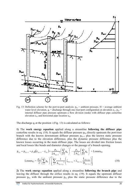
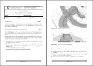
Fig. 13: Definition scheme for the port-to-port analysis: p a,i = ambient pressure, H = average ambient water level elevation, q i = discharge through one riser/port configuration at elevation z j,i . p d,i = internal diffuser pipe pressure upstream a flow division (node) with diffuser pipe centerline elevation z d,i and horizontal pipe location x d,i The discharge q i at the position i (Fig. 13) is calculated as follows: 1) The work energy equation applied along a streamline following the diffuser pipe centerline results in eq. (18). It equals the diffuser pressure p d,i directly upstream the port/riser branch with the known downstream diffuser pressure p d,i-1 plus the known static pressure difference due to the elevation difference, plus the dynamic pressure difference plus the known losses occurring in the main diffuser pipe. The losses are divided into friction losses and local losses like bends and diameter changes or the passage of a branch opening. p i−1 2 i ρe ⎛ ⎞ ρ e ⎛ d, i = p d,i− 1 + ρeg( z d,i−1 − z d,i ) + ⎜ q 2 ∑ k ⎟ − ⎜ q 2 ∑ k 2A d,i 1 ⎝ k 1 ⎠ 2A − = d,i ⎝ k= 1 Losses d,i = ρe ⎛ ⎜ 2 ⎝ i−1 ∑ k= 1 q k 2 ⎞ ⎟ ⎠ ⎡ ⎢ ⎢⎣ ⎛ ⎜ζ ⎝ n d,i −1 1 d,i−1, j ∑ − + λ 2 d,i 1, j d,i−1, j j= 1 A D d,i−1, j d,i−1, j L ⎟ ⎠ ⎞ 2 + Losses d,i 2) The work energy equation applied along a streamline following the branch pipe and leaving the diffuser through the orifice results in eq. (19). It equals the upstream diffuser pressure p d,i with the ambient pressure p a,i plus the static pressure difference due to the ⎞⎤ ⎟ ⎥ ⎠⎥⎦ (18) Institut für Hydromechanik, Universität Karlsruhe 29
elevation difference between diffuser centerline and jet centerline, plus dynamic pressure difference between the diffuser and one single jet plus the losses occurring in all pipe segments between these points. p d,i = p ( ) ( ) i 2 ρe 2 ρe ⎛ ⎞ α 2 iqi − ⎜ q 2 k ⎟ C A 2Ad,i ⎝ k= 1 ⎠ a,i + ρeg(z jet,i − zd,i ) + ∑ ρeq Losses i = 2 2 i ⎡ ⎢ ⎢ ⎣ n p,i ∑ j= 1 2 ⎛ ⎜ α ⎝ A i p,i, j c,i 2 p,i ⎞ ⎛ ⎟ ⎜ζ ⎠ ⎝ p,i, j λ p,i, jL + D p,i, j p,i, j ⎞ ⎟ + ⎠ n r ,i ∑ j= 1 ⎛ ⎜ ⎝ 1 A r,i, j + Losses i 2 ⎞ ⎛ ⎟ ⎜ζ ⎠ ⎝ r,i, j λ r,i, jL + D C c,i denotes the jet contraction coefficient either given by the user or calculated iteratively if Duckbill Valves are applied C c,i,DBV = α i q i / (V DBV,i A p,i ) with V DBV,i = duckbill jet velocity dependent on discharge. If multiple ports are applied a single jet discharge is q jet,i = α i q i with α i = 1/(number of ports at a riser at position i). Solving eq. (18) = (19) for an individual discharge q i gives i−1 2 nd ,i−1 2 ⎛ ⎞ 1 1 Ld,i− 1,j ( p − ) ( − ) ∑ ⎢ ∑ ⎜ ⎟ d,i 1 − pa,i + 2g zd,i 1 − z jet,i + ⎜ qk ⎟ + ζ − + λ 2 2 d,i 1,j d,i−1,j ⎥ ρ e ⎝ k= 1 ⎠ ⎢⎣ Ad,i− 1 j= 1 A − ⎝ D d,i 1,j d,i− j ⎠⎥ q = 1, ⎦ (20) i 2 2 2 np,i n α ⎛ ⎞ ⎛ λ ⎞ r ,i ⎛ ⎞ ⎛ λ ⎞ i ( ) ∑⎜ αi p,i,jLp,i,j r,i,j r,i,j + ⎟ ⎜ζ + ⎟ + ∑⎜ 1 L ⎟ ⎜ζ + ⎟ 2 p,i,j r,i,j C c,iAp,i j= 1 A p,i,j Dp,i, j j= 1 A r,i,j Dr,i, j ⎝ ⎠ ⎝ ⎡ For simple diffusers equation (20) reduces to equation (21) if no risers and no port configurations are applied and the diffuser is just represented by simple holes in the pipe wall. Equation (21) is the one presented in Fischer et al., 1979 which has been used for simple diffuser calculations. i−1 2 ⎡ n −1 2 ⎛ ⎞ 1 d,i 1 ⎛ L ⎞⎤ d,i− j q = ( − ) + ⎜∑ ⎟ ⎢ + ∑ ⎜ζ + λ 1, ⎟ i C c,iA p,i p d,i−1 p a,i q ⎥ (21) k 2 2 ρ ⎝ ⎠ ⎢ d,i−1, j d,i−1, j e k= 1 = ⎣A d,i−1 j 1 A d,i−1, j ⎝ D d,i−1, j ⎠⎥⎦ Fischer et al. (1979) defined a loss coefficient C c,i for sharp-edged entrances: ⎠ ⎝ ⎠ ⎝ ⎛ r,i, j ⎠ r,i, j ⎞⎤ ⎟⎥ ⎠⎥ ⎦ ⎞⎤ (19) C c,i ⎛ 0.58 ⎜⎛ = 0.63 − ⎜⎜ 2g ⎝ ⎝ i−1 ∑ k= 1 q k 2 ⎞ ⎟ ⎠ ⎡ 1 ⎢ ⎢⎣ A d,i 2 −1 ⎤⎛ ⎜ 2 ⎥ ⎥ ⎜ ⎦ ρ ⎝ e ( p − p ) d,i−1 a,i ⎛ + ⎜ ⎝ i−1 ∑ k= 1 q k 2 ⎞ ⎟ ⎠ ⎡ 1 ⎢ ⎢⎣ A d,i 2 −1 ⎤⎞ ⎥ ⎟ ⎥⎟ ⎦⎠ −1 ⎞ ⎟ ⎟ ⎠ and for bell-mouthed ports: C c,i ⎛ ⎜ = 0.975⎜1 − ⎝ 1 2g ⎛ ⎜ ⎝ i−1 ∑ k= 1 q k 2 ⎞ ⎟ ⎠ ⎡ 1 ⎢ ⎢⎣ A 2 d,i−1 ⎤⎛ ⎜ 2 ⎥ ⎥ ⎜ ⎦ ρ ⎝ e ( p − p ) d,i−1 a,i ⎛ + ⎜ ⎝ i−1 ∑ k= 1 q k 2 ⎞ ⎟ ⎠ ⎡ 1 ⎢ ⎢⎣ A 2 d,i−1 ⎤⎞ ⎥⎟ ⎥⎟ ⎦⎠ −1 ⎞ ⎟ ⎟ ⎠ 3 / 8 CorHyd furthermore allows to apply Duckbill valves also on simple diffuser systems and therefore uses the previously defined additional local loss formulations, which are additionally integrated in the calculations of the coefficient C c . Institut für Hydromechanik, Universität Karlsruhe 30
Page 1 and 2: Universität Karlsruhe Institut fü
Page 3 and 4: Acknowledgments The authors like to
Page 5 and 6: 10.1 Local loss formulations: Divis
Page 7 and 8: 1 Introduction CorHyd is a computer
Page 9 and 10: Fig. 1: Outfall configuration showi
Page 11 and 12: where j 0 denotes the buoyancy flux
Page 13 and 14: 2.4 Manifold processes Pipe hydraul
Page 15 and 16: Fig. 8: Local port/riser branch los
Page 17 and 18: Table 2: Local loss formulations Ty
Page 19 and 20: Gradual contraction (Idelchik 1986)
Page 21 and 22: Where H denotes the headloss, V duc
Page 23 and 24: Table 3: Equivalent sand roughness
Page 25 and 26: Institut für Hydromechanik, Univer
Page 27 and 28: For a constant sea water level and
Page 29 and 30: (16) solved for r in (15) and assum
Page 31: 3.1.4 Automatic implementation of l
Page 35 and 36: The iteration stops if the differen
Page 37 and 38: Table 4: CorHyd subroutines and the
Page 39 and 40: 4 Data Input Input can either be do
Page 41 and 42: (ρ 0,max > ρ 0 ). Further sensiti
Page 43 and 44: should allow for riser velocities,
Page 45 and 46: Fig. 19: First input sub-window for
Page 47 and 48: 10 7050.000 0.000 -2.500 11 7000.00
Page 49 and 50: Fig. 22: Graphical output: Energy a
Page 51 and 52: given dilution requirements and maj
Page 53 and 54: 6.3 Off design conditions It was co
Page 55 and 56: Table 5: Sensitivity of involved pa
Page 57 and 58: Fig. 24: Side view and cross sectio
Page 59 and 60: Fig. 27: Flow characteristics for d
Page 61 and 62: under different flow conditions. Th
Page 63 and 64: Fig. 32: Side view and cross sectio
Page 65 and 66: Fig. 34: Flow characteristics for:
Page 71 and 72: Table 6: Comparison of construction
Page 73 and 74: seaward end, which can be prevented
Page 75 and 76: Especially for this long diffuser a
Page 77 and 78: Jirka, G.H., Doneker, R.L. and Hint
Page 79 and 80: 10 Annex 10.1 Local loss formulatio
Page 81 and 82: Institut für Hydromechanik, Univer
Page 83 and 84:
Institut für Hydromechanik, Univer
show all

user's manual for corhyd: an internal diffuser hydraulics model - IfH

You also want an ePaper? Increase the reach of your titles

Delete template?

Save as template?