Centroids, Clusters and Crime: Anchoring the Geographic Profiles of ...

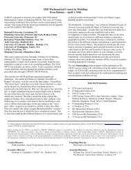
Team # 7507 Page 19
Figure 4: Heat Map showing cratering technique applied to the crime sequence of Peter Sutcliffe
7.1.4 Adjust for Temporal Trends
We would also like our prediction to account for any radial trend in time (the criminal becoming
more bold and committing a crime closer or further away from home). Some research has
suggested that an outward or inward trend in r i may suggest that the next crime will follow this
trend[8]. To accomplish this, we let ˜X = X + △r where △r = rn − r n−1 . We note that this
new random variable, ˜X, gives our intended temporal adjustment in expected value:
E[ ˜X] =E[X + △r] =E[X]+△r
7.2 Results and Analysis
To evaluate this first method, we feed it data from three serial rape sprees. Since the mechanisms
of the model were developed before these data-sets were collected and debugging was
done with different data-sets entirely, we can consider this a blind test.
In each test case, we remove the data point representing the chronologically last crime, and
produce a likelihood surface Z(x, y). As outlined above, we then identify the actual location
of the final crime and compute the standard effectiveness multiplier κ s for each case.
Our first test data-set, coded as “Offender C,” is a comparative success for the model (Figure
5). With k s = 12.19, it is a full order of magnitude better to distribute police resources
using this model instead of distributing uniformly (although it should be remembered that the
absolute size of this number is somewhat more arbitrary for our data than it would be if the
maximum search area had been defined intuitively by a cop familiar with the region).
Qualitatively, one can see the reason for the high κ s : the next crime does indeed on the
surface of our ”crater,” and falls satisfyingly near the isoline of maximum height. Nevertheless,