Slope stability along active and passive continental margins ... - E-LIB

1 Introduction
The conductivity value was then converted to permeability K (m 2 ) using the following equation:
Where μ is viscosity (0.0008Pa×s), ρ is density of water (1.02 g/cm 3 ).
k
K (1.22)
g
Permeability anisotropy r k is commonly defined as the ratio of the hydraulic conductivity parallel to the
bedding plane (i.e., horizontal flow), k h , to the hydraulic conductivity in the direction perpendicular to
the bedding plane (i.e., vertical flow), k v .
rk kh kv
(1.23)
The samples were trimmed to a height of about 7 cm and a diameter of 3.57 cm. ASTM 5084-03
standard was used as guidelines for general procedures (ASTM 2003). Different effective stress values
up to 140 kPa were applied on the samples to monitor the change of the coefficient of permeability at
different depth levels.
Through Terzaghi’s theory of one-dimensional consolidation, the coefficient of permeability (k) can
also be calculated by equation following using consolidation test results:
k cv mv
w
(1.24)
Where m v is the coefficient of volume compressibility (m 2 /MN), defined as the volume change per unit
volume per unit increase in effective stress. If, for an increase in effective stress form σ’ 0 to σ’ 1 , the
void ratio decrease from e 0 to e 1 , then
m
1
e
e
0 1
v
1 e0 '
1
'
0
(1.25)
c v is the coefficient of consolidation (m 2 /year). Since k and mv are assumed as constants, c v is constant
during consolidation. The log time method (Casagrande method) was used to determine c v (Craig
2004):
2
0.196
d
cv
(1.26)
t
Where d is half of the average thickness of the specimen for the particular pressure increment, t 50 is the
time consuming when arriving at the half point for primary consolidation (more detail see Craig 2004).
50
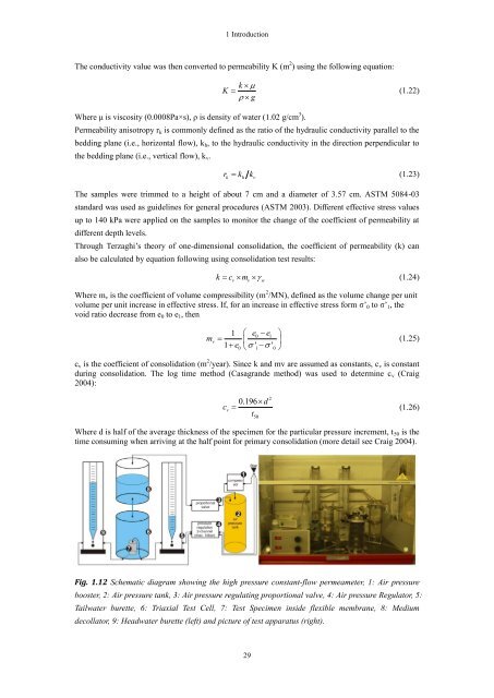
Fig. 1.12 Schematic diagram showing the high pressure constant-flow permeameter, 1: Air pressure
booster, 2: Air pressure tank, 3: Air pressure regulating proportional valve, 4: Air pressure Regulator, 5:
Tailwater burette, 6: Triaxial Test Cell, 7: Test Specimen inside flexible membrane, 8: Medium
decollator, 9: Headwater burette (left) and picture of test apparatus (right).
29