Modeling hemodynamic response for analysis of functional MRI time ...
Modeling hemodynamic response for analysis of functional MRI time ...
Modeling hemodynamic response for analysis of functional MRI time ...

Create successful ePaper yourself
Turn your PDF publications into a flip-book with our unique Google optimized e-Paper software.
HDMF <strong>of</strong> f<strong>MRI</strong> Time-Series <br />
where F( l ) T1 i0 f T (t)e ill and l 2l/T. l represents<br />
the lth harmonic <strong>of</strong> the fundamental frequency<br />
l 2/T <strong>of</strong> the <strong>time</strong>-series. The f T (t) represents the<br />
average period <strong>of</strong> the periodic function f(t) with a<br />
period T. Because the experimental design determines<br />
X( l ), the set <strong>of</strong> equations defined by Eq. (8) can be<br />
utilized to determine the optimal parameters <strong>of</strong> the<br />
HDMF, h(t). The standard approach is to attempt to<br />
find the 2 -fitting or weighted least-square estimation<br />
which minimizes the cost function 2 [Press et al., 1994]:<br />
T1<br />
2 t1<br />
(Y( l )<br />
H( l )X( l ))*(Y( l ) H( l )X( l ))/ l<br />
2<br />
(9)<br />
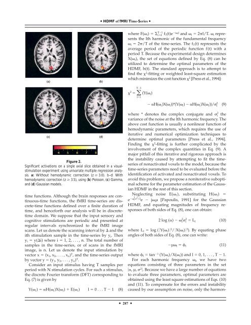
Figure 2.<br />
Significant activations on a single axial slice obtained in a visualstimulation<br />
experiment using univariate multiple regression <strong>analysis</strong>.<br />
a: Without <strong>hemodynamic</strong> correction (z 3.0). b–d: With<br />
<strong>hemodynamic</strong> correction (z 3.5), using (b) Poisson, (c) Gamma,<br />
and (d) Gaussian models.<br />
<strong>time</strong> functions. Although the brain <strong>response</strong>s are continuous-<strong>time</strong><br />
functions, the f<strong>MRI</strong> <strong>time</strong>-series are discrete-<strong>time</strong><br />
functions defined over a finite duration <strong>of</strong><br />
<strong>time</strong>, and hence<strong>for</strong>th our <strong>analysis</strong> will be in discrete<strong>time</strong><br />
domain. We suppose that the input sensory and<br />
cognitive stimulations are periodic and presented at<br />
regular intervals synchronized to the f<strong>MRI</strong> image<br />
scans. Let us denote the scanning interval by and the<br />
ith stimulation sample in the <strong>time</strong>-series by y i . Then<br />
y i y(i) where i 1,2,...,n.Thetotal number <strong>of</strong><br />
samples in the <strong>time</strong>-series, or <strong>of</strong> scans in the f<strong>MRI</strong><br />
image, is n. Let us denote the input stimulation by<br />
vector x (x 1 ,x 2 ,...,x n ) T , and the <strong>time</strong>-series output<br />
by vector y (y 1 ,y 2 ,...,y n ) T .<br />
Consider an input stimulus having T samples per<br />
period with N stimulation cycles. For such a stimulus,<br />
the discrete Fourier trans<strong>for</strong>m (DFT) corresponding to<br />
Eq. (7) is given by<br />
Y( l ) H( l )X( l ) E( l ) l0...T1 (8)<br />
where * denotes the complex conjugate and 2<br />
l the<br />
variance <strong>of</strong> the noise at the lth harmonic frequency. The<br />
above cost function is usually a nonlinear function <strong>of</strong><br />
<strong>hemodynamic</strong> parameters, which requires the use <strong>of</strong><br />
iterative and numerical optimization techniques to<br />
determine optimal parameters [Press et al., 1994].<br />
Finding the 2 -fitting is further complicated by the<br />
involvement <strong>of</strong> the complex quantities in Eq. (9). A<br />
major pitfall <strong>of</strong> this iterative and rigorous approach is<br />
the instability caused by attempting to fit the <strong>time</strong>series<br />
<strong>of</strong> nonactivated voxels to the model, because the<br />
<strong>time</strong>-series parameters need to be evaluated be<strong>for</strong>e the<br />
identification <strong>of</strong> activated and nonactivated voxels. To<br />
avoid this problem, we propose a noniterative suboptimal<br />
scheme <strong>for</strong> the parameter estimation <strong>of</strong> the Gaussian<br />
HDMF in the rest <strong>of</strong> this section.<br />
Neglecting noise E( l ), substituting H( l ) <br />
e 2<br />
l <br />
2 /2<br />
e j l µ [Papoulis, 1991] <strong>for</strong> the Gaussian<br />
HDMF, and equating magnitudes <strong>of</strong> frequency <strong>response</strong>s<br />
<strong>of</strong> both sides <strong>of</strong> Eq. (8), one can obtain:<br />
2 log () l 2 l 2 L l (10)<br />
where L l log (0Y( l )0 2 /0X( l )0 2 ). By equating phase<br />
angles <strong>of</strong> both sides <strong>of</strong> Eq. (8), one can write:<br />
µ l l (11)<br />
where l tan 1 (Y( l )/X( l )) and l 0,1,...,T1.<br />
For each harmonic frequency l , we have two<br />
equations consisting <strong>of</strong> three parameters in the set<br />
5, µ, 2 6. Because we have a large number <strong>of</strong> equations<br />
to evaluate three parameters, optimal parameters are<br />
obtained using the least square estimations <strong>of</strong> Eqs. (10)<br />
and (11). To compensate <strong>for</strong> the errors and instability<br />
caused by our assumption on noise, only the harmon-<br />
287