Modeling hemodynamic response for analysis of functional MRI time ...

Rajapakse et al.
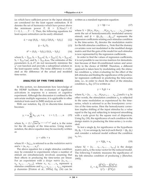
ics which have sufficient power in the input stimulus
are considered for the least square estimation. If
denotes the set of harmonics which have power above
the minimum power P, 5l;0X( l )0 2 P,
l 0,1,...,T16. Then, the following equations for
least-square estimation can be easily obtained:
ˆ exp 5(S 3 S 4 S 5 S 2 )/2(S 1 S 4 S 2 S 2 )6 (12)
µˆ S 6 /S 2 (13)
ˆ 2 (S 3 S 2 S 5 S 2 )/(S 1 S 4 S 2 S 2 ) (14)
where S 1 l ,S 2 l l 2 ,S 3 l L l 2 ,S 4 l l 4 ,
S 5 l L l l 2 , and S 6 l 1 l . The estimates of the
parameters 5ˆ,µˆ,ˆ26 do not necessarily minimize the
2 cost function and provide a suboptimal solution in
the least-squares sense. The noise difference is evaluated
as the difference of the actual and modeled
time-series.
ANALYSIS OF FMRI TIME-SERIES
In this section, we demonstrate how knowledge of
the HDMF facilitates the evaluation of significant
activations in response to a sensory or cognitive
experiment. Although the discussion is confined to the
univariate multiple regression, it is applicable to other
statistical tests used in fMRI analysis as well.
With our notation, Eq. (2) in discrete-time domain
becomes:
n
y i l1
h i(il) x l i i1,2,...,n (15)
where h ij (1/2 2 )e (ijµ)2 /2 2 and i is the noise
for the ith sample of the time-series. Using matrix
notation, the above equation may be succinctly written
as
y Hx (16)
where H 5h ij 6 nxn is referred to as the modulation matrix
and ( 1 , 2 ,..., n ) T .
The above equation for a single stimulus condition
may be extended to experiments where a number of
stimuli are simultaneously involved, assuming that
their effects in producing the time-series are linear.
For an experiment with a design matrix [x 1 ,x 2 ,...
x q , x q1 ,...,x qp ], where x 1 , x 2 ,...,x q represent q
stimulus conditions and x q1 ,x q2 ,..., x qp represent
p dummies [Friston et al., 1995a], Eq. (16) can be
written as a standard regression equation:
y X (17)
where X [H 1 x 1 ,H 2 x 2 ,...,H q x q ,x q1 ,...,x qp ] represents
the set of hemodynamically modulated sensory
stimuli, and ( 1 , 2 ,..., qp ) T represents the
regression coefficients relating each stimulus condition
to the time-series. H k denotes the modulation matrix
for the kth stimulus condition x k . Note that the dummy
covariates were not modulated in the modified design
matrix and that the gain of the model for each stimulus
is now represented by the regression coefficients.
In order to find the values of regression coefficients,
it is not possible to use inverse matrices for demodulation
because of their ill-conditioned nature and sensitivity
to the choice of HDMF. Therefore, a different
approach is taken here by modulating only the stimulus
condition x k when evaluating for the effect of the
kth stimulus and finding the significance of the particular
regression coefficient in predicting the time-series
data, i.e., in order to check the effect of the stimulus
condition x k , Eq. (17) is written as
y X k (18)
where X k [x 1 ...x k1 H k x k x k1 ...x pq ] and k q. In
other words, the stimulation condition x k is subjected
to the same modulation as experienced by the timeseries,
which is referred to as the hemodynamic correction
of the time-series. Here the hemodynamic correction
implies shifting of the input stimulus by a value
equal to the lag and subjecting to temporal smoothing
with a scale given by the square root of dispersion.
Using Eq. (18), the significance of each condition in the
design matrix in producing the time-series y is evaluated.
To test a single k for significance or the hypothesis
H 0 : k 0, we arrange k last in such that ( k , k )
and consider a reduced model without the condition
x k , i.e.,
y X* k k k (19)
where X* k [x 1 ...x k1 x k1 ...x pq ] is the design
matrix and k is the noise vector for the reduced model.
The following F-statistic measures the significance of
the kth stimulus condition of producing y [Rencher,
1995]:
(ˆ T X T k y ˆk
T X* kT y)
F k d k
(y T y ˆT X T k y)
(20)
288