arXiv:hep-th/9304011 v1 Apr 5 1993
arXiv:hep-th/9304011 v1 Apr 5 1993
arXiv:hep-th/9304011 v1 Apr 5 1993

Create successful ePaper yourself
Turn your PDF publications into a flip-book with our unique Google optimized e-Paper software.
It is extremely interesting to note <strong>th</strong>at — even for pure gravity — <strong>th</strong>e <strong>th</strong>ird quantized<br />
universe propagator is not <strong>th</strong>e naive minisuperspace Wheeler–DeWitt propagator (5.20).<br />
In particular <strong>th</strong>e ultraviolet behavior of <strong>th</strong>e propagator (in E) is completely different from<br />
<strong>th</strong>e naive propagator (5.20). For example, <strong>th</strong>e 1/E 2 behavior in <strong>th</strong>e ultraviolet becomes<br />
e −πE behavior. Our understanding of why <strong>th</strong>is is so is incomplete. (Part of <strong>th</strong>e story is<br />
explained in <strong>th</strong>e next section.)<br />
In general, we can decompose amplitudes as<br />
〈<br />
W (l1 ) · · · W (l n ) 〉 ∫ ∏<br />
=<br />
i<br />
dE i ψ Ei<br />
(l i ) A(E 1 , . . . , E n ) , (10.22)<br />
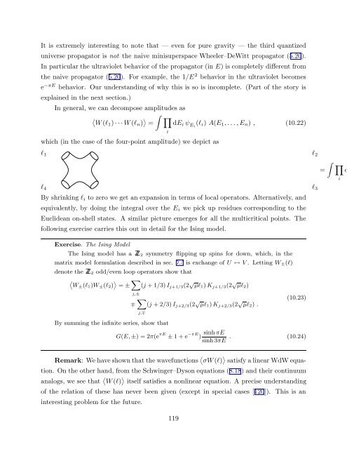
which (in <strong>th</strong>e case of <strong>th</strong>e four-point amplitude) we depict as<br />
l 1<br />
l 2<br />
∫ ∏<br />
=<br />
i<br />
l 4 l 3<br />
By shrinking l i to zero we get an expansion in terms of local operators. Alternatively, and<br />
equivalently, by doing <strong>th</strong>e integral over <strong>th</strong>e E i we pick up residues corresponding to <strong>th</strong>e<br />
Euclidean on-shell states. A similar picture emerges for all <strong>th</strong>e multicritical points. The<br />
following exercise carries <strong>th</strong>is out in detail for <strong>th</strong>e Ising model.<br />
d<br />
Exercise. The Ising Model<br />
The Ising model has a Z 2 symmetry flipping up spins for down, which, in <strong>th</strong>e<br />
matrix model formulation described in sec. 7.5 is exchange of U ↔ V . Letting W ± (l)<br />
denote <strong>th</strong>e Z 2 odd/even loop operators show <strong>th</strong>at<br />
〈<br />
W± (l 1 )W ± (l 2 ) 〉 ∑<br />
= ± (j + 1/3) I j+1/3 (2 √ µl 1 ) K j+1/3 (2 √ µl 2 )<br />
j,±<br />
∑<br />
∓ (j + 2/3) I j+2/3 (2 √ µl 1 ) K j+2/3 (2 √ µl 2 ) .<br />
j,∓<br />
(10.23)<br />
By summing <strong>th</strong>e infinite series, show <strong>th</strong>at<br />
G(E, ±) = 2π(e πE ± 1 + e −πE sinh πE<br />
)<br />
sinh 3πE . (10.24)<br />
Remark: We have shown <strong>th</strong>at <strong>th</strong>e wavefunctions 〈 σW (l) 〉 satisfy a linear WdW equation.<br />
On <strong>th</strong>e o<strong>th</strong>er hand, from <strong>th</strong>e Schwinger–Dyson equations (8.18) and <strong>th</strong>eir continuum<br />
analogs, we see <strong>th</strong>at 〈 W (l) 〉 itself satisfies a nonlinear equation. A precise understanding<br />
of <strong>th</strong>e relation of <strong>th</strong>ese has never been given (except in special cases [120]). This is an<br />
interesting problem for <strong>th</strong>e future.<br />
119