- Page 1 and 2: YCTP-P23-92 LA-UR-92-3479 hep-th/93
- Page 3 and 4: 7.1. Orthogonal polynomials . . . .
- Page 5 and 6: contexts. The aim of these lectures
- Page 7 and 8: 1) As Quantum Gravity In this guise
- Page 9 and 10: semiclassical, and quantum Liouvill
- Page 11 and 12: The Lagrangian and Hamiltonian form
- Page 13 and 14: mation, on an annulus. This is give
- Page 15 and 16: Quantum mechanically, we try to und
- Page 17 and 18: about the domain of integration. Th
- Page 19 and 20: diffeomorphism invariance, (2.11) s
- Page 21 and 22: quantum gravity [31], so it would b
- Page 23 and 24: To determine ∆, we employ the sam
- Page 25 and 26: The stress-energy tensor following
- Page 27 and 28: Note that the uniformizing map (3.1
- Page 29 and 30: In particular, passing from the pla
- Page 31 and 32: Exercise. The wall analogy Show tha
- Page 33 and 34: Here ν is a real number. An import
- Page 35 and 36: 5) As will be seen in sec. 5.4 belo
- Page 37 and 38: where ∆ i is the conformal weight
- Page 39 and 40: where j k ≡ −α k /γ. Strictly
- Page 41 and 42: where |Σ〉 is a state created by
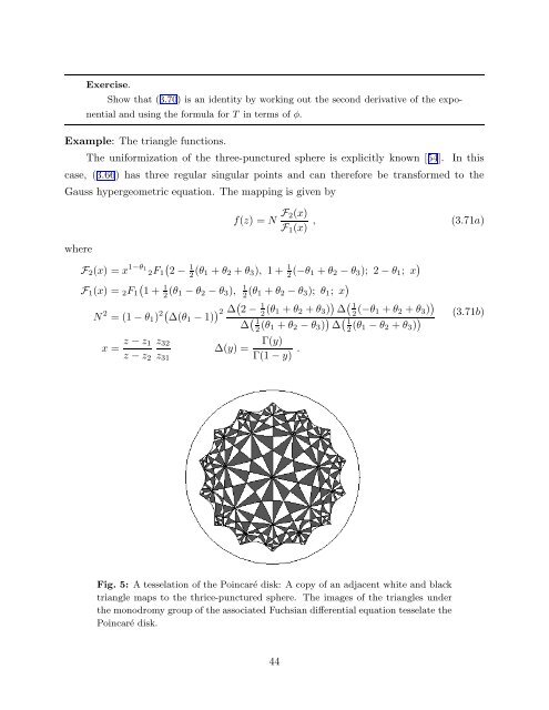
- Page 43: equation with sources, (3.42). We s
- Page 47 and 48: In view of these observations, the
- Page 49 and 50: 3.11. Surfaces with boundaries The
- Page 51 and 52: 4. 2D Euclidean Quantum Gravity II:
- Page 53 and 54: 4.3. KPZ states in 2D Quantum Gravi
- Page 55 and 56: In the KP formalism of the matrix m
- Page 57 and 58: In fact, the c = 1 model has much m
- Page 59 and 60: We may plot the quantum numbers of
- Page 61 and 62: On the RHS we have one, rather than
- Page 63 and 64: 5.1. Particles in D Dimensions: QFT
- Page 65 and 66: where H is the Wheeler-DeWitt opera
- Page 67 and 68: Euclidean signature spacetimes. The
- Page 69 and 70: 5.4. 2D String Theory: Minkowskian
- Page 71 and 72: 2) The only difference in degrees o
- Page 73 and 74: Those who look for special states i
- Page 75 and 76: Fig. 10: The case of the exploding
- Page 77 and 78: Fig. 11: A piece of a random triang
- Page 79 and 80: Since ∂ /2 eJ2 ∂J = Je J2 /2 ,
- Page 81 and 82: (6.8). As familiar from field theor
- Page 83 and 84: continuum, as reviewed in preceding
- Page 85 and 86: 7. Matrix Model Technology I: Metho
- Page 87 and 88: with r n a scalar coefficient indep
- Page 89 and 90: gravity. It is natural that pure gr
- Page 91 and 92: with α = 1 10 . The solution to (7
- Page 93 and 94: parameters to result in a (2l−1)
- Page 95 and 96:
and the recursion relations for thi
- Page 97 and 98:
The formal expansion of Q l−1/2 =
- Page 99 and 100:
If we consider the higher operators
- Page 101 and 102:
of the symmetry factor for the Feyn
- Page 103 and 104:
1) The expansions in V and ζ −1
- Page 105 and 106:
V′ ( ) + + + . . . ∂ ∂L L =
- Page 107 and 108:
and the main observation is 〈∏
- Page 109 and 110:
2 λ Fig. 17: The Wigner semicircle
- Page 111 and 112:
Example. The Gaussian potential We
- Page 113 and 114:
Exercise. Using the asymptotics of
- Page 115 and 116:
The formulae (10.1) and (10.2), whi
- Page 117 and 118:
10.2. Loops to Local Operators By s
- Page 119 and 120:
This suggests that instead of the l
- Page 121 and 122:
Fig. 20: Two loops on a continuum s
- Page 123 and 124:
Using Feynman diagrams to obtain th
- Page 125 and 126:
continuous and particle states are
- Page 127 and 128:
Here λ 1,2 are the two turning poi
- Page 129 and 130:
As we have seen from the tree-level
- Page 131 and 132:
Laplace transform the eigenvalue de
- Page 133 and 134:
The perturbative expansion of the H
- Page 135 and 136:
11.5. Wavefunctions and Wheeler-DeW
- Page 137 and 138:
x Fig. 24: The function x 2 K 0 (x)
- Page 139 and 140:
Remarks: 1) The definition (11.59)
- Page 141 and 142:
p λ Fig. 25: A generic initial con
- Page 143 and 144:
anches can very well evolve into on
- Page 145 and 146:
It follows that if we define a nonl
- Page 147 and 148:
12.5. The w ∞ Symmetry of the Har
- Page 149 and 150:
The w ∞ symmetry of the inverted
- Page 151 and 152:
coadjoint orbit quantization for a
- Page 153 and 154:
egarded as space, the time coordina
- Page 155 and 156:
The equivalence of the collective f
- Page 157 and 158:
Kondo effect, the Callan-Rubakov ef
- Page 159 and 160:
13.4. Tree-Level Collective Field T
- Page 161 and 162:
presence of a wall. The function R
- Page 163 and 164:
ω q R(µ + ω ; V ) R q q > 0 −
- Page 165 and 166:
Property (i) follows from the integ
- Page 167 and 168:
The key observation is that the com
- Page 169 and 170:
(13.44) is given by F = F 0 + 1 µ
- Page 171 and 172:
and in (13.51) we only keep terms t
- Page 173 and 174:
e) The c = 1 model is equivalent to
- Page 175 and 176:
The expansion is only convergent fo
- Page 177 and 178:
Example. Let us consider the most g
- Page 179 and 180:
free-field techniques. But this cal
- Page 181 and 182:
Quite generally, the operator produ
- Page 183 and 184:
x p−1 ∼ y q−1 ∼ 1 (where C(
- Page 185 and 186:
spin j even at the self-dual radius
- Page 187 and 188:
15.2. Disappointments From the quan
- Page 189 and 190:
We thank especially N. Seiberg for
- Page 191 and 192:
References [1] M. B. Green and J. S
- Page 193 and 194:
[36] G. Moore, N. Seiberg, and M. S
- Page 195 and 196:
[76] S.R. Das and A. Jevicki, “St
- Page 197 and 198:
Phys. B368 (1992) 671; S. Jain and
- Page 199 and 200:
[145] E. Martinec and S. Shatashvil