arXiv:hep-th/9304011 v1 Apr 5 1993

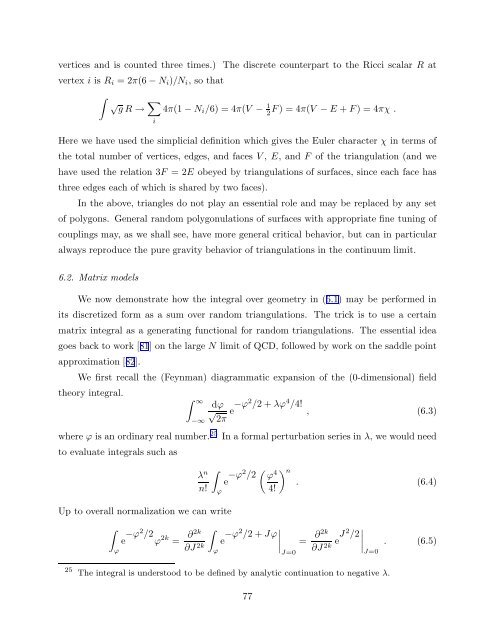
vertices and is counted three times.) The discrete counterpart to the Ricci scalar R at
vertex i is R i = 2π(6 − N i )/N i , so that
∫ √g R →
∑
i
4π(1 − N i /6) = 4π(V − 1 F ) = 4π(V − E + F ) = 4πχ .
2
Here we have used the simplicial definition which gives the Euler character χ in terms of
the total number of vertices, edges, and faces V , E, and F of the triangulation (and we
have used the relation 3F = 2E obeyed by triangulations of surfaces, since each face has
three edges each of which is shared by two faces).
In the above, triangles do not play an essential role and may be replaced by any set
of polygons. General random polygonulations of surfaces with appropriate fine tuning of
couplings may, as we shall see, have more general critical behavior, but can in particular
always reproduce the pure gravity behavior of triangulations in the continuum limit.
6.2. Matrix models
We now demonstrate how the integral over geometry in (6.1) may be performed in
its discretized form as a sum over random triangulations. The trick is to use a certain
matrix integral as a generating functional for random triangulations. The essential idea
goes back to work [81] on the large N limit of QCD, followed by work on the saddle point
approximation [82].
We first recall the (Feynman) diagrammatic expansion of the (0-dimensional) field
theory integral.
∫ ∞
−∞
dϕ
√
2π
e −ϕ2 /2 + λϕ 4 /4! , (6.3)
where ϕ is an ordinary real number. 25 In a formal perturbation series in λ, we would need
to evaluate integrals such as
λ n
n!
Up to overall normalization we can write
∫
ϕ
e −ϕ2 /2 ϕ 2k =
∂2k
∫
∂J 2k ∫ϕ
ϕ
e −ϕ2 /2 ( ϕ 4 ) n
. (6.4)
4!
e −ϕ2 /2 + Jϕ ∣ ∣ ∣∣
J=0
= ∂2k
∂J 2k eJ 2 /2 ∣ ∣
∣∣J=0 . (6.5)
25 The integral is understood to be defined by analytic continuation to negative λ.
77