SPEX User's Manual - SRON
SPEX User's Manual - SRON
SPEX User's Manual - SRON

You also want an ePaper? Increase the reach of your titles
YUMPU automatically turns print PDFs into web optimized ePapers that Google loves.
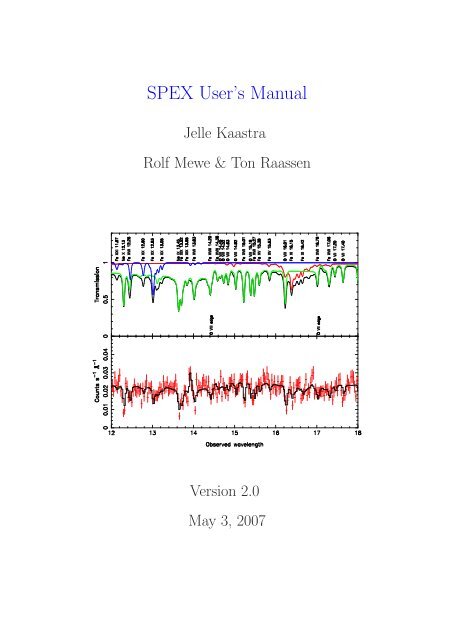
<strong>SPEX</strong> User’s <strong>Manual</strong><br />
Jelle Kaastra<br />
Rolf Mewe & Ton Raassen<br />
Version 2.0<br />
May 3, 2007
Contents<br />
1 Introduction 7<br />
1.1 Preface . . . . . . . . . . . . . . . . . . . . . . . . . . . . . . . . . . . . . . . . . 7<br />
1.2 Sectors and regions . . . . . . . . . . . . . . . . . . . . . . . . . . . . . . . . . . . 7<br />
1.2.1 Introduction . . . . . . . . . . . . . . . . . . . . . . . . . . . . . . . . . . 7<br />
1.2.2 Sky sectors . . . . . . . . . . . . . . . . . . . . . . . . . . . . . . . . . . . 8<br />
1.2.3 Detector regions . . . . . . . . . . . . . . . . . . . . . . . . . . . . . . . . 8<br />
1.3 Different types of spectral components . . . . . . . . . . . . . . . . . . . . . . . . 8<br />
2 Syntax overview 11<br />
2.1 Abundance: standard abundances . . . . . . . . . . . . . . . . . . . . . . . . . . 11<br />
2.2 Ascdump: ascii output of plasma properties . . . . . . . . . . . . . . . . . . . . . 13<br />
2.3 Bin: rebin the spectrum . . . . . . . . . . . . . . . . . . . . . . . . . . . . . . . . 15<br />
2.4 Calculate: evaluate the spectrum . . . . . . . . . . . . . . . . . . . . . . . . . . . 15<br />
2.5 Comp: create, delete and relate spectral components . . . . . . . . . . . . . . . . 16<br />
2.6 Data: read response file and spectrum . . . . . . . . . . . . . . . . . . . . . . . . 17<br />
2.7 DEM: differential emission measure analysis . . . . . . . . . . . . . . . . . . . . 18<br />
2.8 Distance: set the source distance . . . . . . . . . . . . . . . . . . . . . . . . . . . 20<br />
2.9 Egrid: define model energy grids . . . . . . . . . . . . . . . . . . . . . . . . . . . 22<br />
2.10 Elim: set flux energy limits . . . . . . . . . . . . . . . . . . . . . . . . . . . . . . 23<br />
2.11 Error: Calculate the errors of the fitted parameters . . . . . . . . . . . . . . . . . 24<br />
2.12 Fit: spectral fitting . . . . . . . . . . . . . . . . . . . . . . . . . . . . . . . . . . . 25<br />
2.13 Ibal: set type of ionisation balance . . . . . . . . . . . . . . . . . . . . . . . . . . 26<br />
2.14 Ignore: ignoring part of the spectrum . . . . . . . . . . . . . . . . . . . . . . . . 27<br />
2.15 Ion: select ions for the plasma models . . . . . . . . . . . . . . . . . . . . . . . . 27<br />
2.16 Log: Making and using command files . . . . . . . . . . . . . . . . . . . . . . . . 28<br />
2.17 Menu: Menu settings . . . . . . . . . . . . . . . . . . . . . . . . . . . . . . . . . . 29<br />
2.18 Model: show the current spectral model . . . . . . . . . . . . . . . . . . . . . . . 30<br />
2.19 Multiply: scaling of the response matrix . . . . . . . . . . . . . . . . . . . . . . . 30<br />
2.20 Obin: optimal rebinning of the data . . . . . . . . . . . . . . . . . . . . . . . . . 31<br />
2.21 Par: Input and output of model parameters . . . . . . . . . . . . . . . . . . . . . 31<br />
2.22 Plot: Plotting data and models . . . . . . . . . . . . . . . . . . . . . . . . . . . . 34<br />
2.23 Quit: finish the program . . . . . . . . . . . . . . . . . . . . . . . . . . . . . . . . 38<br />
2.24 Sector: creating, copying and deleting of a sector . . . . . . . . . . . . . . . . . . 38<br />
2.25 Shiftplot: shift the plotted spectrum for display purposes . . . . . . . . . . . . . 39<br />
2.26 Simulate: Simulation of data . . . . . . . . . . . . . . . . . . . . . . . . . . . . . 40<br />
2.27 Step: Grid search for spectral fits . . . . . . . . . . . . . . . . . . . . . . . . . . . 41<br />
2.28 Syserr: systematic errors . . . . . . . . . . . . . . . . . . . . . . . . . . . . . . . . 42
4 CONTENTS<br />
2.29 System . . . . . . . . . . . . . . . . . . . . . . . . . . . . . . . . . . . . . . . . . . 43<br />
2.30 Use: reuse part of the spectrum . . . . . . . . . . . . . . . . . . . . . . . . . . . . 43<br />
2.31 Var: various settings for the plasma models . . . . . . . . . . . . . . . . . . . . . 44<br />
2.31.1 Overview . . . . . . . . . . . . . . . . . . . . . . . . . . . . . . . . . . . . 44<br />
2.31.2 Syntax . . . . . . . . . . . . . . . . . . . . . . . . . . . . . . . . . . . . . . 45<br />
2.31.3 Examples . . . . . . . . . . . . . . . . . . . . . . . . . . . . . . . . . . . . 45<br />
2.32 Vbin: variable rebinning of the data . . . . . . . . . . . . . . . . . . . . . . . . . 45<br />
2.33 Watch . . . . . . . . . . . . . . . . . . . . . . . . . . . . . . . . . . . . . . . . . . 46<br />
3 Spectral Models 49<br />
3.1 Overview of spectral components . . . . . . . . . . . . . . . . . . . . . . . . . . . 49<br />
3.2 Absm: Morrison & McCammon absorption model . . . . . . . . . . . . . . . . . . 49<br />
3.3 Bb: Blackbody model . . . . . . . . . . . . . . . . . . . . . . . . . . . . . . . . . 49<br />
3.4 Cf: isobaric cooling flow differential emission measure model . . . . . . . . . . . . 51<br />
3.5 Cie: collisional ionisation equilibrium model . . . . . . . . . . . . . . . . . . . . . 51<br />
3.5.1 Temperatures . . . . . . . . . . . . . . . . . . . . . . . . . . . . . . . . . . 51<br />
3.5.2 Line broadening . . . . . . . . . . . . . . . . . . . . . . . . . . . . . . . . 52<br />
3.5.3 Density effects . . . . . . . . . . . . . . . . . . . . . . . . . . . . . . . . . 52<br />
3.5.4 Non-thermal electron distributions . . . . . . . . . . . . . . . . . . . . . . 52<br />
3.5.5 Abundances . . . . . . . . . . . . . . . . . . . . . . . . . . . . . . . . . . . 52<br />
3.5.6 Parameter description . . . . . . . . . . . . . . . . . . . . . . . . . . . . . 53<br />
3.6 Dbb: Disk blackbody model . . . . . . . . . . . . . . . . . . . . . . . . . . . . . . 53<br />
3.7 Delt: delta line model . . . . . . . . . . . . . . . . . . . . . . . . . . . . . . . . . 54<br />
3.8 Dem: Differential Emission Measure model . . . . . . . . . . . . . . . . . . . . . 55<br />
3.9 Dust: dust scattering model . . . . . . . . . . . . . . . . . . . . . . . . . . . . . . 55<br />
3.10 Etau: simple transmission model . . . . . . . . . . . . . . . . . . . . . . . . . . . 56<br />
3.11 Euve: EUVE absorption model . . . . . . . . . . . . . . . . . . . . . . . . . . . . 56<br />
3.12 File: model read from a file . . . . . . . . . . . . . . . . . . . . . . . . . . . . . . 57<br />
3.13 Gaus: Gaussian line model . . . . . . . . . . . . . . . . . . . . . . . . . . . . . . 57<br />
3.14 Hot: collisional ionisation equilibrium absorption model . . . . . . . . . . . . . . 58<br />
3.15 Knak: segmented power law transmission model . . . . . . . . . . . . . . . . . . 58<br />
3.16 Laor: Relativistic line broadening model . . . . . . . . . . . . . . . . . . . . . . . 59<br />
3.17 Lpro: Spatial broadening model . . . . . . . . . . . . . . . . . . . . . . . . . . . . 59<br />
3.18 Mbb: Modified blackbody model . . . . . . . . . . . . . . . . . . . . . . . . . . . 60<br />
3.19 Neij: Non-Equilibrium Ionisation Jump model . . . . . . . . . . . . . . . . . . . . 61<br />
3.20 Pdem: DEM models . . . . . . . . . . . . . . . . . . . . . . . . . . . . . . . . . . 61<br />
3.20.1 Short description . . . . . . . . . . . . . . . . . . . . . . . . . . . . . . . . 61<br />
3.21 Pow: Power law model . . . . . . . . . . . . . . . . . . . . . . . . . . . . . . . . . 62<br />
3.22 Reds: redshift model . . . . . . . . . . . . . . . . . . . . . . . . . . . . . . . . . . 63<br />
3.23 Refl: Reflection model . . . . . . . . . . . . . . . . . . . . . . . . . . . . . . . . . 64<br />
3.24 Rrc: Radiative Recombination Continuum model . . . . . . . . . . . . . . . . . . 64<br />
3.25 Spln: spline continuum model . . . . . . . . . . . . . . . . . . . . . . . . . . . . . 65<br />
3.26 Vblo: Rectangular velocity broadening model . . . . . . . . . . . . . . . . . . . . 66<br />
3.27 Vgau: Gaussian velocity broadening model . . . . . . . . . . . . . . . . . . . . . 67<br />
3.28 Vpro: Velocity profile broadening model . . . . . . . . . . . . . . . . . . . . . . . 67<br />
3.29 Wdem: power law differential emission measure model . . . . . . . . . . . . . . . 68
CONTENTS 5<br />
4 More about plotting 69<br />
4.1 Plot devices . . . . . . . . . . . . . . . . . . . . . . . . . . . . . . . . . . . . . . . 69<br />
4.2 Plot types . . . . . . . . . . . . . . . . . . . . . . . . . . . . . . . . . . . . . . . . 69<br />
4.3 Plot colours . . . . . . . . . . . . . . . . . . . . . . . . . . . . . . . . . . . . . . . 70<br />
4.4 Plot line types . . . . . . . . . . . . . . . . . . . . . . . . . . . . . . . . . . . . . 72<br />
4.5 Plot text . . . . . . . . . . . . . . . . . . . . . . . . . . . . . . . . . . . . . . . . . 73<br />
4.5.1 Font types (font) . . . . . . . . . . . . . . . . . . . . . . . . . . . . . . . . 73<br />
4.5.2 Font heights (fh) . . . . . . . . . . . . . . . . . . . . . . . . . . . . . . . . 74<br />
4.5.3 Special characters . . . . . . . . . . . . . . . . . . . . . . . . . . . . . . . 74<br />
4.6 Plot captions . . . . . . . . . . . . . . . . . . . . . . . . . . . . . . . . . . . . . . 76<br />
4.7 Plot symbols . . . . . . . . . . . . . . . . . . . . . . . . . . . . . . . . . . . . . . 77<br />
4.8 Plot axis units and scales . . . . . . . . . . . . . . . . . . . . . . . . . . . . . . . 78<br />
4.8.1 Plot axis units . . . . . . . . . . . . . . . . . . . . . . . . . . . . . . . . . 78<br />
4.8.2 Plot axis scales . . . . . . . . . . . . . . . . . . . . . . . . . . . . . . . . . 78<br />
5 Response matrices 83<br />
5.1 Respons matrices . . . . . . . . . . . . . . . . . . . . . . . . . . . . . . . . . . . . 83<br />
5.2 Introduction . . . . . . . . . . . . . . . . . . . . . . . . . . . . . . . . . . . . . . . 83<br />
5.3 Data binning . . . . . . . . . . . . . . . . . . . . . . . . . . . . . . . . . . . . . . 84<br />
5.3.1 Introduction . . . . . . . . . . . . . . . . . . . . . . . . . . . . . . . . . . 84<br />
5.3.2 The Shannon theorem . . . . . . . . . . . . . . . . . . . . . . . . . . . . . 84<br />
5.3.3 Integration of Shannon’s theorem . . . . . . . . . . . . . . . . . . . . . . . 85<br />
5.3.4 The χ 2 test . . . . . . . . . . . . . . . . . . . . . . . . . . . . . . . . . . . 86<br />
5.3.5 Extension to complex spectra . . . . . . . . . . . . . . . . . . . . . . . . . 88<br />
5.3.6 Difficulties with the χ 2 test . . . . . . . . . . . . . . . . . . . . . . . . . . 89<br />
5.3.7 The Kolmogorov-Smirnov test . . . . . . . . . . . . . . . . . . . . . . . . 90<br />
5.3.8 Examples . . . . . . . . . . . . . . . . . . . . . . . . . . . . . . . . . . . . 92<br />
5.3.9 Final remarks . . . . . . . . . . . . . . . . . . . . . . . . . . . . . . . . . . 94<br />
5.4 Model binning . . . . . . . . . . . . . . . . . . . . . . . . . . . . . . . . . . . . . 95<br />
5.4.1 Model energy grid . . . . . . . . . . . . . . . . . . . . . . . . . . . . . . . 95<br />
5.4.2 Evaluation of the model spectrum . . . . . . . . . . . . . . . . . . . . . . 96<br />
5.4.3 Binning the model spectrum . . . . . . . . . . . . . . . . . . . . . . . . . 97<br />
5.4.4 Which approximation to choose? . . . . . . . . . . . . . . . . . . . . . . . 99<br />
5.4.5 The effective area . . . . . . . . . . . . . . . . . . . . . . . . . . . . . . . . 100<br />
5.4.6 Final remarks . . . . . . . . . . . . . . . . . . . . . . . . . . . . . . . . . . 101<br />
5.5 The proposed response matrix . . . . . . . . . . . . . . . . . . . . . . . . . . . . . 101<br />
5.5.1 Dividing the response into components . . . . . . . . . . . . . . . . . . . . 101<br />
5.5.2 More complex situations . . . . . . . . . . . . . . . . . . . . . . . . . . . . 102<br />
5.5.3 A response component . . . . . . . . . . . . . . . . . . . . . . . . . . . . . 103<br />
5.6 Determining the grids in practice . . . . . . . . . . . . . . . . . . . . . . . . . . . 105<br />
5.6.1 Creating the data bins . . . . . . . . . . . . . . . . . . . . . . . . . . . . . 105<br />
5.6.2 creating the model bins . . . . . . . . . . . . . . . . . . . . . . . . . . . . 106<br />
5.7 Proposed file formats . . . . . . . . . . . . . . . . . . . . . . . . . . . . . . . . . . 107<br />
5.7.1 Proposed response format . . . . . . . . . . . . . . . . . . . . . . . . . . . 107<br />
5.7.2 Proposed spectral file format . . . . . . . . . . . . . . . . . . . . . . . . . 109<br />
5.8 examples . . . . . . . . . . . . . . . . . . . . . . . . . . . . . . . . . . . . . . . . 111<br />
5.8.1 Introduction . . . . . . . . . . . . . . . . . . . . . . . . . . . . . . . . . . 111<br />
5.8.2 Rosat PSPC . . . . . . . . . . . . . . . . . . . . . . . . . . . . . . . . . . 112
6 CONTENTS<br />
5.8.3 ASCA SIS0 . . . . . . . . . . . . . . . . . . . . . . . . . . . . . . . . . . . 112<br />
5.8.4 XMM RGS data . . . . . . . . . . . . . . . . . . . . . . . . . . . . . . . . 115<br />
5.9 References . . . . . . . . . . . . . . . . . . . . . . . . . . . . . . . . . . . . . . . . 116<br />
6 Installation and testing 119<br />
6.1 Testing the software . . . . . . . . . . . . . . . . . . . . . . . . . . . . . . . . . . 119<br />
7 Acknowledgements 121<br />
7.1 Acknowledgements . . . . . . . . . . . . . . . . . . . . . . . . . . . . . . . . . . . 121
Chapter 1<br />
Introduction<br />
1.1 Preface<br />
At the time of releasing version 2.0 of the code, the full documentation is not yet available,<br />
although major parts have been completed (you are reading that part now). This manual will<br />
be extended during the coming months. Check the version you have (see the front page for<br />
the date it was created). In the mean time, there are several useful hints and documentation<br />
available at the web site of Alex Blustin (MSSL), who I thank for his help in this. That web<br />
site can be found at:<br />
http://www.mssl.ucl.ac.uk/ ajb/spex/spex.html<br />
The official <strong>SPEX</strong> website is:<br />
http://www.sron.nl/divisions/hea/spex/index.html<br />
We apologize for the temporary inconvenience.<br />
1.2 Sectors and regions<br />
1.2.1 Introduction<br />
In many cases an observer analysis the observed spectrum of a single X-ray source. There are<br />
however situations with more complex geometries.<br />
Example 1: An extended source, where the spectrum may be extracted from different regions<br />
of the detector, but where these spectra need to be analysed simultaneously due to the overlap<br />
in point-spread function from one region to the other. This situation is e.g. encountered in the<br />
analysis of cluster data with ASCA or BeppoSAX.<br />
Example 2: For the RGS detector of XMM-Newton, the actual data-space in the dispersion<br />
direction is actually two-dimensional: the position z where a photon lands on the detector and<br />
its energy or pulse height E as measured with the CCD detector. X-ray sources that are extended<br />
in the direction of the dispersion axis φ are characterised by spectra that are a function of both<br />
the energy E and off-axis angle φ. The sky photon distribution as a function of (φ,E) is then<br />
mapped onto the (z,E)-plane. By defining appropriate regions in both planes and evaluating<br />
the correct (overlapping) responses, one may analyse extended sources.<br />
Example 3: One may also fit simultaneously several time-dependent spectra using the same<br />
response, e.g. data obtained during a stellar flare.<br />
It is relatively easy to model all these situations (provided that the instrument is understood<br />
sufficiently, of course), as we show below.
8 Introduction<br />
1.2.2 Sky sectors<br />
First, the relevant part of the sky is subdivided into sectors, each sector corresponding to a<br />
particular region of the source, for example a circular annulus centered around the core of a<br />
cluster, or an arbitrarily shaped piece of a supernova remnant, etc.<br />
A sector may also be a point-like region on the sky. For example if there is a bright point source<br />
superimposed upon the diffuse emission of the cluster, we can define two sectors: an extended<br />
sector for the cluster emission, and a point-like sector for the point source. Both sectors might<br />
even overlap, as this example shows!<br />
Another example: the two nearby components of the close binary α Centauri observed with<br />
the XMM -Newton instruments, with overlapping point-spread-functions of both components.<br />
In that case we would have two point-like sky sectors, each sector corresponding to one of the<br />
double star’s components.<br />
The model spectrum for each sky sector may and will be different in general. For example, in<br />
the case of an AGN superimposed upon a cluster of galaxies, one might model the spectrum of<br />
the point-like AGN sector using a power law, and the spectrum from the surrounding cluster<br />
emission using a thermal plasma model.<br />
1.2.3 Detector regions<br />
The observed count rate spectra are extracted in practice in different regions of the detector.<br />
It is necessary here to distinguish clearly the (sky) sectors and (detector) regions. A detector<br />
region for the XMM EPIC camera would be for example a rectangular box, spanning a certain<br />
number of pixels in the x- and y-directions. It may also be a circular or annular extraction region<br />
centered around a particular pixel of the detector, or whatever spatial filter is desired. For the<br />
XMM RGS it could be a specific ”banana” part of the detector-coordinate CCD pulse-height<br />
plane (z,E).<br />
Note that the detector regions need not to coincide with the sky sectors, neither should their<br />
number to be equal! A good example of this is again the example of an AGN superimposed<br />
upon a cluster of galaxies. The sky sector corresponding to the AGN is simply a point, while,<br />
for a finite instrumental psf, its extraction region at the detector is for example a circular region<br />
centered around the pixel corresponding to the sky position of the source.<br />
Also, one could observe the same source with a number of different instruments and analyse the<br />
data simultaneously. In this case one would have only one sky sector but more detector regions,<br />
namely one for each participating instrument.<br />
1.3 Different types of spectral components<br />
In a spectral model <strong>SPEX</strong> uses two different types of components, called additive and multiplicative<br />
components respectively. Additive components have a normalisation that determines the<br />
flux level. Multiplicative components operate on additive components. A delta line or a power<br />
law are typical examples of additive components. Interstellar absorption is a typical example of<br />
multiplicative components.<br />
The redshift component is treated as a multiplicative component, since it operates on additive<br />
components.<br />
Additive components can be divided into two classes: simple components (like power law, blackbody<br />
etc.) and plasma components, that use our atomic code. For the plasma components it is<br />
possible to plot or list specific properties, while for the simple models this is not applicable.
1.3 Different types of spectral components 9<br />
Multiplicative components can be divided into 3 classes. First, there are the absorption-type<br />
components, like interstellar absorption. These components simply are an energy-dependent<br />
multiplication of the original source spectrum. <strong>SPEX</strong> has both simple absorption components<br />
as well as absorption components based upon our plasma code. The second class consists of<br />
shifts: redshift (either due to Doppler shifts or due to cosmology) is the prototype of this. The<br />
third class consists of convolution-type operators. An example is Gaussian velocity broadening.<br />
For more information about the currently defined spectral components in <strong>SPEX</strong>, see chapter 3.
10 Introduction
Chapter 2<br />
Syntax overview<br />
2.1 Abundance: standard abundances<br />
Overview<br />
For the plasm models, a default set of abundances is used. All abundances are calculated relative<br />
to those standard values. The current default abundance set is Anders & Grevesse ([1989]).<br />
However, it is recommended to use the more recent compilation by Lodders ([2003]). In particular<br />
we recommend to use the proto-solar (= solar system) abundances for most applications,<br />
as the solar photospheric abundance has been affected by nucleosynthesis (burning of H to He)<br />
and settlement in the Sun during its lifetime. The following abundances (Table 2.1) can be used<br />
in <strong>SPEX</strong>:<br />
Table 2.1: Standard abundance sets<br />
Abbrevation Reference<br />
reset default (=Anders & Grevesse)<br />
ag Anders & Grevesse ([1989])<br />
allen Allen ([1973])<br />
ra Ross & Aller ([1976])<br />
grevesse Grevesse et al. ([1992])<br />
gs Grevesse & Sauval ([1998])<br />
lodders Lodders proto-solar ([2003])<br />
solar Lodders solar photospheric ([2003])<br />
For the case of Grevesse & Sauval (1998) we adopted their meteoritic values (in general more<br />
accurate than the photospheric values, but in most cases consistent), except for He (slightly<br />
enhanced in the solar photosphere due to element migration at the bottom of the convection<br />
zone), C, N and O (largely escaped from meteorites) Ne and Ar (noble gases).<br />
In Table 2.2 we show the values of the standard abundances. They are expressed in logarithmic<br />
units, with hydrogen by definition 12.0. For Allen ([1973]) the value for boron is just an upper<br />
limit.<br />
Warning: For Allen ([1973]) the value for boron is just an upper limit.<br />
Syntax<br />
The following syntax rules apply:
12 Syntax overview<br />
Table 2.2: Abundances for the standard sets<br />
Z elem AG Allen RA Grevesse GS Lodders solar<br />
1 H 12.00 12.00 12.00 12.00 12.00 12.00 12.00<br />
2 He 10.99 10.93 10.80 10.97 10.99 10.98 10.90<br />
3 Li 1.16 0.70 1.00 1.16 3.31 3.35 3.28<br />
4 Be 1.15 1.10 1.15 1.15 1.42 1.48 1.41<br />
5 B 2.6 ¡3.0 2.11 2.6 2.79 2.85 2.78<br />
6 C 8.56 8.52 8.62 8.55 8.52 8.46 8.39<br />
7 N 8.05 7.96 7.94 7.97 7.92 7.90 7.83<br />
8 O 8.93 8.82 8.84 8.87 8.83 8.76 8.69<br />
9 F 4.56 4.60 4.56 4.56 4.48 4.53 4.46<br />
10 Ne 8.09 7.92 7.47 8.08 8.08 7.95 7.87<br />
11 Na 6.33 6.25 6.28 6.33 6.32 6.37 6.30<br />
12 Mg 7.58 7.42 7.59 7.58 7.58 7.62 7.55<br />
13 Al 6.47 6.39 6.52 6.47 6.49 6.54 6.46<br />
14 Si 7.55 7.52 7.65 7.55 7.56 7.61 7.54<br />
15 P 5.45 5.52 5.50 5.45 5.56 5.54 5.46<br />
16 S 7.21 7.20 7.20 7.21 7.20 7.26 7.19<br />
17 Cl 5.5 5.60 5.50 5.5 5.28 5.33 5.26<br />
18 Ar 6.56 6.90 6.01 6.52 6.40 6.62 6.55<br />
19 K 5.12 4.95 5.16 5.12 5.13 5.18 5.11<br />
20 Ca 6.36 6.30 6.35 6.36 6.35 6.41 6.34<br />
21 Sc 1.10 1.22 1.04 3.20 3.10 3.15 3.07<br />
22 Ti 4.99 5.13 5.05 5.02 4.94 5.00 4.92<br />
23 V 4.00 4.40 4.02 4.00 4.02 4.07 4.00<br />
24 Cr 5.67 5.85 5.71 5.67 5.69 5.72 5.65<br />
25 Mn 5.39 5.40 5.42 5.39 5.53 5.58 5.50<br />
26 Fe 7.67 7.60 7.50 7.51 7.50 7.54 7.47<br />
27 Co 4.92 5.10 4.90 4.92 4.91 4.98 4.91<br />
28 Ni 6.25 6.30 6.28 6.25 6.25 6.29 6.22<br />
29 Cu 4.21 4.50 4.06 4.21 4.29 4.34 4.26<br />
30 Zn 4.60 4.20 4.45 4.60 4.67 4.70 4.63<br />
abundance #a - Set the standard abundances to the values of reference #a in the table above.<br />
Examples<br />
abundance gs - change the standard abundances to the set of Grevesse & Sauval ([1998])<br />
abundance reset - reset the abundances to the standard set
2.2 Ascdump: ascii output of plasma properties 13<br />
2.2 Ascdump: ascii output of plasma properties<br />
Overview<br />
One of the drivers in developing <strong>SPEX</strong> is the desire to be able to get insight into the astrophysics<br />
of X-ray sources, beyond merely deriving a set of best-fit parameters like temperature or<br />
abundances. The general user might be interested to know ionic concentrations, recombination<br />
rates etc. In order to facilitate this <strong>SPEX</strong> contains options for ascii-output.<br />
Ascii-output of plasma properties can be obtained for any spectral component that uses the<br />
basic plasma code of <strong>SPEX</strong>; for all other components (like power law spectra, gaussian lines,<br />
etc.) this sophistication is not needed and therefore not included. There is a choice of properties<br />
that can be displayed, and the user can either display these properties on the screen or write it<br />
to file.<br />
The possible output types are listed below. Depending on the specific spectral model, not all<br />
types are allowed for each spectral component. The keyword in front of each item is the one<br />
that should be used for the appropriate syntax.<br />
plas: basic plasma properties like temperature, electron density etc.<br />
abun: elemental abundances and average charge per element.<br />
icon: ion concentrations, both with respect to Hydrogen and the relevant elemental abundance.<br />
rate: total ionization, recombination and charge-transfer rates specified per ion.<br />
rion: ionization rates per atomic subshell, specified according to the different contributing processes.<br />
pop: the occupation numbers as well as upwards/downwards loss and gain rates to all quantum<br />
levels included.<br />
elex: the collisional excitation and de-excitation rates for each level, due to collisions with<br />
electrons.<br />
prex: the collisional excitation and de-excitation rates for each level, due to collisions with<br />
protons.<br />
rad: the radiative transition rates from each level.<br />
two: the two-photon emission transition rates from each level.<br />
grid: the energy and wavelength grid used in the last evaluation of the spectrum.<br />
clin: the continuum, line and total spectrum for each energy bin for the last plasma layer of<br />
the model.<br />
line: the line energy and wavelength, as well as the total line emission (photons/s) for each line<br />
contributing to the spectrum, for the last plasma layer of the model.<br />
con: list of the ions that contribute to the free-free, free-bound and two-photon continuum<br />
emission, followed by the free-free, free-bound, two-photon and total continuum spectrum,<br />
for the last plasma layer of the model.
14 Syntax overview<br />
tcl: the continuum, line and total spectrum for each energy bin added for all plasma layers of<br />
the model.<br />
tlin: the line energy and wavelength, as well as the total line emission (photons/s) for each line<br />
contributing to the spectrum, added for all plasma layers of the model.<br />
tcon: list of the ions that contribute to the free-free, free-bound and two-photon continuum<br />
emission, followed by the free-free, free-bound, two-photon and total continuum spectrum,<br />
added for all plasma layers of the model.<br />
cnts: the number of counts produced by each line. Needs an instrument to be defined before.<br />
snr: hydrodynamical and other properties of the supernova remnant (only for supernova remnant<br />
models such as Sedov, Chevalier etc.).<br />
heat: plasma heating rates (only for photoionized plasmas).<br />
ebal: the energy balance contributions of each layer (only for photoionized plasmas).<br />
dem: the emission measure distribution (for the pdem model)<br />
col: the ionic column densities for the hot, pion, slab, xabs and warm models<br />
tran: the transmission and equivalent width of absorption lines and absorption edges for the<br />
hot, pion, slab, xabs and warm models<br />
warm: the column densities, effective ionization parameters and temperatures of the warm<br />
model<br />
Syntax<br />
The following syntax rules apply for ascii output:<br />
ascdump terminal #i1 #i2 #a - Dump the output for sky sector #i1 and component #i2 to<br />
the terminal screen; the type of output is described by the parameter #a which is listed in the<br />
table above.<br />
ascdump file #a1 #i1 #i2 #a2 - As above, but output written to a file with its name given by<br />
the parameter #a1. The suffix ”.asc” will be appended automatically to this filename.<br />
Warning: Any existing files with the same name will be overwritten.<br />
Examples<br />
ascdump terminal 3 2 icon - dumps the ion concentrations of component 2 of sky sector 3 to<br />
the terminal screen.<br />
ascdump file mydump 3 2 icon - dumps the ion concentrations of component 2 of sky sector<br />
3 to a file named mydump.asc.
2.3 Bin: rebin the spectrum 15<br />
2.3 Bin: rebin the spectrum<br />
Overview<br />
This command rebins the data (thus both the spectrum file and the response file) in a manner<br />
as described in Sect. 2.6. The range to be rebinned can be specified either as a channel range<br />
(no units required) or in eiter any of the following units: keV, eV, Rydberg, Joule, Hertz, Å,<br />
nanometer, with the following abbrevations: kev, ev, ryd, j, hz, ang, nm.<br />
Syntax<br />
The following syntax rules apply:<br />
bin #r #i - This is the simplest syntax allowed. One needs to give the range, #r, over at least<br />
the input data channels one wants to rebin. If one wants to rebin the whole input file the range<br />
must be at least the whole range over data channels (but a greater number is also allowed). #i<br />
is then the factor by which the data will be rebinned.<br />
bin [instrument #i1] [region #i2] #r #i - Here one can also specify the instrument and region<br />
to be used in the binning. This syntax is necessary if multiple instruments or regions are used<br />
in the data input.<br />
bin [instrument #i1] [region #i2] #r #i [unit #a] - In addition to the above here one can also<br />
specify the units in which the binning range is given. The units can be eV, Å, or any of the<br />
other units specified above.<br />
Examples<br />
bin 1:10000 10 - Rebins the input data channel 1:10000 by a factor of 10.<br />
bin instrument 1 1:10000 10 - Rebins the data from the first instrument as above.<br />
bin 1:40 10 unit a - Rebins the input data between 1 and 40 Å by a factor of 10.<br />
2.4 Calculate: evaluate the spectrum<br />
Overview<br />
This command evaluates the current model spectrum. When one or more instruments are<br />
present, it also calculates the model folded through the instrument. Whenever the user has<br />
modified the model or its parameters manually, and wants to plot the spectrum or display<br />
model parameters like the flux in a given energy band, this command should be executed first<br />
(otherwise the spectrum is not updated). On the other hand, if a spectral fit is done (by typing<br />
the ”fit” command) the spectrum will be updated automatically and the calculate command<br />
needs not to be given.<br />
Syntax<br />
The following syntax rules apply:<br />
calc - Evaluates the spectral model.
16 Syntax overview<br />
Examples<br />
calc - Evaluates the spectral model.<br />
2.5 Comp: create, delete and relate spectral components<br />
Overview<br />
In fitting or evaluating a spectrum, one needs to build up a model made out of at least 1<br />
component. This set of commands can create a new component in the model, as well as delete<br />
any component. Usually we distinguish two types of spectral components in <strong>SPEX</strong>.<br />
The additive components correspond to emission components, such as a power law, a Gaussian<br />
emission line, a collisional ionization equilibrium (CIE) component, etc.<br />
The second class (dubbed here multiplicative components for ease) consists of operations to be<br />
applied to the additive components. Examples are truly multiplicative operations, such as the<br />
Galactic absorption, where the model spectrum of any additive component should be multiplied<br />
by the transmission of the absorbing interstellar medium, warm absorbers etc. Other operations<br />
contained in this class are redshifts, convolutions with certain velocity profiles, etc.<br />
The user needs to define in <strong>SPEX</strong> which multiplicative component should be applied to which<br />
additive components, and in which order. The order is important as operations are not always<br />
communative. This setting is also done with this component command.<br />
If multiple sectors are present in the spectral model or response matrix (see Sect. 1.2) then<br />
one has to specify the spectral components and their relation for each sector. The possible<br />
components to the model are listed and described in Sect. 3.<br />
Note that the order that you define the components is not important. However, for each sector,<br />
the components are numbered starting from 1, and these numbers should be used when relating<br />
the multiplicative components to the additive components.<br />
If you want to see the model components and the way they are related, type ”model show”.<br />
Warning: If in any of the commands as listed above you omit the sector number or sector<br />
number range, the operation will be done for all sectors that are present. For example, having<br />
3 sectors, the ”comp pow” command will define a power law component for each of the three<br />
sectors. If you only want to define/delete/relate the component for one sector, you should specify<br />
the sector number(s). In the very common case that you have only one sector you can always<br />
omit the sector numbers.<br />
Warning: After deleting a component, all components are re-numbered! So if you have components<br />
1,2,3 for example as pow, cie, gaus, and you type ”comp del 2”, you are left with 1=pow,<br />
2=gaus.<br />
Syntax<br />
The following syntax rules apply:<br />
comp [#i:] #a - Creates a component #a as part of the model for the (optional) sector range<br />
#i:<br />
comp delete [#i1:] #i2: - Deletes the components with number from range #i2: for sector range<br />
(optional) #i1. See also the warning above<br />
comp relation [#i1:] #i2: #i3,...,#in - Apply multiplicative components #i3, ..., #in (numbers)<br />
in this order, to the additive components given in the range #i2: of sectors in the range
2.6 Data: read response file and spectrum 17<br />
#i1 (optional). Note that the multiplicative components must be separated by a ”,”<br />
Examples<br />
comp pow - Creates a power-law component for modeling the spectrum for all sectors that are<br />
present.<br />
comp 2 pow - Same as above, but now the component is created for sector 2.<br />
comp 4:6 pow - Create the power law for sectors 4, 5 and 6<br />
com abs - Creates a Morrison & McCammon absorption component.<br />
comp delete 2 - Deletes the second created component. For example, if you have 1 = pow, 2<br />
= cie and 3 = gaus, this command delets the cie component and renumbers 1 = pow, 2 = gaus<br />
comp del 1:2 - In the example above, this will delete the pow and cie components and renumbers<br />
now 1 = gaus<br />
comp del 4:6 2 - If the above three component model (pow, cie, gaus) would be defined for 8<br />
sectors (numbered 1–8), then this command deletes the cie component (nr. 2) for sectors 4–6<br />
only.<br />
comp rel 1 2 - Apply component 2 to component 1. For example, if you have defined before<br />
with ”comp pow” and ”comp ”abs” a power law and galactic absorption, the this command tells<br />
you to apply component 2 (abs) to component 1 (pow).<br />
comp rel 1 5,3,4 - Taking component 1 a power law (pow), component 3 a redshift operation<br />
(reds), component 4 galactic absorption (abs) and component 5 a warm absorber (warm), this<br />
command has the effect that the power law spectrum is multiplied first by the transmission of<br />
the warm absorber (5=warm), then redshifted (3=reds) and finally multiplied by the transmission<br />
of our galaxy (4=abs). Note that the order is always from the source to the observer!<br />
comp rel 1:2 5,3,4 - Taking component 1 a power law (pow), component 2 a gaussian line<br />
(gaus), and 3–5 as above, this model applies multiplicative components 5, 3 and 4 (in that orer)<br />
to the emission spectra of both component 1 (pow) and 2 (cie).<br />
comp rel 7:8 1:2 5,3,4 - As above, but only for sectors 7 and 8 (if those are defined)<br />
2.6 Data: read response file and spectrum<br />
Overview<br />
In order to fit an observed spectrum, <strong>SPEX</strong> needs a spectral data file and a response matrix.<br />
These data are stored in FITS format, tailored for <strong>SPEX</strong> (see section 5.7). The data files need<br />
not necessarily be located in the same directory, one can also give a pathname plus filename in<br />
this command.<br />
Syntax<br />
The following syntax rules apply: data #a1 #a2 - Read response matrix #a1 and spectrum<br />
#a2<br />
data delete instrument #i - Remove instrument #i from the data set<br />
data merge sum #i: - Merge instruments in range #i: to a single spectrum and response matrix,<br />
by adding the data and matrices<br />
data merge aver #i: - Merge instruments in range #i: to a single spectrum and response matrix,
18 Syntax overview<br />
by averaging the data and matrices<br />
data save #i #a [overwrite] - Save data #a from instrument #i with the option to overwrite the<br />
existent file. <strong>SPEX</strong> automatically tags the .spo extension to the given file name. No response<br />
file is saved.<br />
data show - Shows the data input given, as well as the count (rates) for source and background,<br />
the energy range for which there is data the response groups and data channels. Also the integration<br />
time and the standard plotting options are given.<br />
Examples<br />
data mosresp mosspec - read a spectral response file named mosresp.res and the corresponding<br />
spectral file mosspec.spo. Hint, although 2 different names are used here for ease of understanding,<br />
it is eased if the spectrum and response file have the same name, with the appropriate<br />
extension.<br />
data delete instrument 1 - delete the first instrument<br />
data merge aver 3:5 - merge instruments 3–5 into a single new instrument 3 (replacing the<br />
old instrument 3), by averaging the spectra. Spectra 3–5 could be spectra taken with the same<br />
instrument at different epochs.<br />
data merge sum 1:2 - add spectra of instruments 1–2 into a single new instrument 1 (replacing<br />
the old instrument 1), by adding the spectra. Useful for example in combining XMM-Newton<br />
MOS1 and MOS2 spectra.<br />
data save 1 mydata - Saves the data from instrument 1 in the working directory under the<br />
filename of mydata.spo<br />
data /mydir/data/mosresp /mydir/data/mosspec - read the spectrum and response from the<br />
directory /mydir/data/<br />
2.7 DEM: differential emission measure analysis<br />
Overview<br />
<strong>SPEX</strong> offers the opportunity to do a differential emission measure analysis. This is an effective<br />
way to model multi-temperature plasmas in the case of continuous temperature distributions or<br />
a large number of discrete temperature components.<br />
The spectral model can only have one additive component: the DEM component that corresponds<br />
to a multi-temperature structure. There are no restrictions to the number of multiplicative<br />
components. For a description of the DEM analysis method see document <strong>SRON</strong>/<strong>SPEX</strong>/TRPB05<br />
(in the documentation for version 1.0 of <strong>SPEX</strong>) Mewe et al. (1994) and Kaastra et al. (1996).<br />
<strong>SPEX</strong> has 5 different dem analysis methods implemented, as listed shortly below. We refer to<br />
the above papers for more details.<br />
1. reg – Regularization method (minimizes second order derivative of the DEM; advantage:<br />
produces error bars; disadvantage: needs fine-tuning with a regularization parameter and<br />
can produce negative emission measures.<br />
2. clean – Clean method: uses the clean method that is widely used in radio astronomy.<br />
Useful for ”spiky emission measure distributions.
2.7 DEM: differential emission measure analysis 19<br />
3. poly – Polynomial method: approximates the DEM by a polynomial in the log T − − log Y<br />
plane, where Y is the emission measure. Works well if the DEM is smooth.<br />
4. mult – Multi-temperature method: tries to fit the DEM to the sum of Gaussian components<br />
as a function of log T. Good for discrete and slightly broadened components, but may not<br />
always converge.<br />
5. gene – Genetic algorithm: using a genetic algorithm try to find the best solution. Advantage:<br />
rather robust for avoiding local subminima.Disadvantage: may require a lot of cpu<br />
time, and each run produces slightly different results (due to randomization).<br />
In practice to use the DEM methods the user should do the following steps:<br />
1. Read and prepare the spectral data that should be analysed<br />
2. Define the dem model with the ”comp dem” command<br />
3. Define any multiplicative models (absorption, redshifts, etc.) that should be applied to<br />
the additive model<br />
4. Define the parameters of the dem model: number of temperature bins, temperature range,<br />
abundances etc.<br />
5. give the ”dem lib” command to create a library of isothermal spectra.<br />
6. do the dem method of choice (each one of the five methods outlined above)<br />
7. For different abundances or parameters of any of the spectral components, first the ”dem<br />
lib” command must be re-issued!<br />
Syntax<br />
The following syntax rules apply:<br />
dem lib - Create the basic DEM library of isothermal spectra<br />
dem reg auto - Do DEM analysis using the regularization method, using an automatic search<br />
of the optimum regularization parameter. It determines the regularisation parameter R in such<br />
a way that χ 2 (R) = χ 2 (0)[1 + s √ 2/(n − n T ] where the scaling factor s = 1, n is the number<br />
of spectral bins in the data set and n T is the number of temperature components in the DEM<br />
library.<br />
dem reg auto #r - As above, but for the scaling factor s set to #r.<br />
dem reg #r - Do DEM analysis using the regularization method, using a fixed regularization<br />
parameter R =#r.<br />
dem chireg #r1 #r2 #i - Do a grid search over the regularization parameter R, with #i steps<br />
and R distributed logarithmically between #r1 and #r2. Useful to scan the χ 2 (R) curve whenever<br />
it is complicated and to see how much ”penalty’ (negative DEM values) there are for each<br />
value of R.<br />
dem clean - Do DEM analysis using the clean method<br />
dem poly #i - Do DEM analysis using the polynomial method, where #i is the degree of the<br />
polynomial<br />
dem mult #i - Do DEM analysis using the multi-temperature method, where #i is the number<br />
of broad components
20 Syntax overview<br />
dem gene #i1 #i2 - Do DEM analysis using the genetic algorithm, using a population size given<br />
by #i1 (maximum value 1024) and #i2 is the number of generations (no limit, in practice after<br />
∼100 generations not much change in the solution. Experiment with these numbers for your<br />
practical case.<br />
dem read #a - Read a DEM distribution from a file named #a which automatically gets the<br />
extension ”.dem”. It is an ascii file with at least two columns, the first column is the temperature<br />
in keV and the second column the differential emission measure, in units of 10 64 m −3 keV −1 .<br />
The maximum number of data points in this file is 8192. Temperature should be in increasing<br />
order. The data will be interpolated to match the temperature grid defined in the dem model<br />
(which is set by the user).<br />
dem save #a - Save the DEM to a file #a with extension ”.dem”. The same format as above is<br />
used for the file. A third column has the corresponding error bars on the DEM as determined<br />
by the DEM method used (not always relevant or well defined, exept for the regularization<br />
method).<br />
dem smooth #r - Smoothes a DEM previously determined by any DEM method using a block<br />
filter/ Here #r is the full width of the filter expressed in 10 log T. Note that this smoothing will<br />
in principle worsen the χ 2 of the solution, but it is sometimes useful to ”wash out” some residual<br />
noise in the DEM distribution, preserving total emission measure.<br />
Examples<br />
dem lib - create the DEM library<br />
dem reg auto - use the automatic regularization method<br />
dem reg 10. - use a regularization parameter of R = 10 in the regularization method<br />
dem chireg 1.e-5 1.e5 11 - do a grid search using 11 regularisation parameters R given by<br />
10 −5 , 10 −4 , 0.001, 0.01, 0.1, 1, 10, 100, 1000, 10 4 , 10 5 .<br />
dem clean - use the clean method<br />
dem poly 7 - use a 7th degree polynomial method<br />
dem gene 512 128 - use the genetic algorithm with a population of 512 and 128 generations<br />
dem save mydem - save the current dem on a file named mydem.dem<br />
dem read modeldem - read the dem from a file named modeldem.dem<br />
dem smooth 0.3 - smooth the DEM to a temperature width of 0.3 in 10 log T (approximately a<br />
factor of 2 in temperature range).<br />
2.8 Distance: set the source distance<br />
Overview<br />
One of the main principles of <strong>SPEX</strong> is that spectral models are in principle calculated at the<br />
location of the X-ray source. Once the spectrum has been evaluated, the flux received at Earth<br />
can be calculated. In order to do that, the distance of the source must be set.<br />
<strong>SPEX</strong> allows for the simultaneous analysis of multiple sky sectors. In each sector, a different<br />
spectral model might be set up, including a different distance. For example, a foreground object<br />
that coincides partially with the primary X-ray source has a different distance value.<br />
The user can specify the distance in a number of different units. Allowed distance units are<br />
shown in the table below.
2.8 Distance: set the source distance 21<br />
Abbrevation<br />
spex<br />
m<br />
au<br />
ly<br />
pc<br />
kpc<br />
mpc<br />
z<br />
cz<br />
Table 2.3: <strong>SPEX</strong> distance units<br />
Unit<br />
internal <strong>SPEX</strong> units of 10 22 m (this is the default)<br />
meter<br />
Astronomical Unit, 1.49597892 10 11 m<br />
lightyear, 9.46073047 10 15 m<br />
parsec, 3.085678 10 16 m<br />
kpc, kiloparsec, 3.085678 10 19 m<br />
Mpc, Megaparsec, 3.085678 10 22 m<br />
redshift units for the given cosmological parameters<br />
recession velocity in km/s for the given cosmological parameters<br />
The default unit of 10 22 m is internally used in all calculations in <strong>SPEX</strong>. The reason is that with<br />
this scaling all calculations ranging from solar flares to clusters of galaxies can be done with<br />
single precision arithmetic, without causing underflow or overflow. For the last two units (z and<br />
cz), it is necessary to specify a cosmological model. Currently this model is simply described by<br />
H 0 , Ω m (matter density), Ω Λ (cosmological constant related density), and Ω r (radiation density).<br />
At startup, the values are:<br />
H 0 : 70 km/s/Mpc ,<br />
Ω m : 0.3 ,<br />
Ω Λ : 0.7 ,<br />
Ω r : 0.0<br />
i.e. a flat model with cosmological constant. However, the user can specify other values of the<br />
cosmological parameters. Note that the distance is in this case the luminosity distance.<br />
Note that the previous defaults for <strong>SPEX</strong> (H 0 = 50, q 0 = 0.5) can be obtained by putting<br />
H 0 = 50, Ω m = 1, Ω Λ = 0 and Ω r = 0.<br />
Warning: when H 0 or any of the Ω is changed, the luminosity distance will not change, but the<br />
equivalent redshift of the source is adjusted. For example, setting the distance first to z=1 with<br />
the default H 0 =70 km/s/Mpc results into a distance of 2.03910 26 m. When H 0 is then changed<br />
to 100 km/s/Mpc, the distance is still 2.16810 26 m, but the redshift is adjusted to 1.3342.<br />
Warning: In the output also the light travel time is given. This should not be confused with<br />
the (luminosity) distance in light years, which is simply calculated from the luminosity distance<br />
in m!<br />
Syntax<br />
The following syntax rules apply to setting the distance:<br />
distance [sector #i:] #r [#a] - set the distance to the value #r in the unit #a. This optional<br />
distance unit may be omittted. In that case it is assumed that the distance unit is the default<br />
<strong>SPEX</strong> unit of 10 22 m. The distance is set for the sky sector range #i:. When the optional sector<br />
range is omitted, the distance is set for all sectors.<br />
distance show - displays the distance in various units for all sectors.<br />
distance h0 #r - sets the Hubble constant H 0 to the value #r.
22 Syntax overview<br />
distance om #r - sets the Ω m parameter to the value #r.<br />
distance ol #r - sets the Ω Λ parameter to the value #r.<br />
distance or #r - sets the Ω r parameter to the value #r.<br />
Examples<br />
distance 2 - sets the distance to 2 default units, i.e. to 2E22 m.<br />
distance 12.0 pc - sets the distance for all sectors to 12 pc.<br />
distance sector 3 0.03 z - sets the distance for sector 3 to a redshift of 0.03.<br />
distance sector 2 : 4 50 ly - sets the distance for sectors 2-4 to 50 lightyear.<br />
distance h0 50. - sets the Hubble constant to 50 km/s/Mpc.<br />
distance om 0.27 - sets the matter density parameter Ω m to 0.27<br />
distance show - displays the distances for all sectors, see the example below for the output<br />
format.<br />
<strong>SPEX</strong>> di 100 mpc<br />
Distances assuming H0 = 70.0 km/s/Mpc, Omega_m = 0.300 Omega_Lambda = 0.700 Omega_r = 0.000<br />
Sector m A.U. ly pc kpc Mpc redshift cz age(yr)<br />
----------------------------------------------------------------------------------------------<br />
1 3.086E+24 2.063E+13 3.262E+08 1.000E+08 1.000E+05 100.0000 0.0229 6878.7 3.152E+08<br />
----------------------------------------------------------------------------------------------<br />
2.9 Egrid: define model energy grids<br />
Overview<br />
<strong>SPEX</strong> operates essentially in two modes: with an observational data set (read using the data commands),<br />
or without data, i.e. theoretical model spectra. In the first case, the energy grid neede to evaluate the<br />
spectra is taken directly from the data set. In the second case, the user can choose his own energy grid.<br />
The energy grid can be a linear grid, a logarithmic grid or an arbitrary grid read from an ascii-file. It<br />
is also possible to save the current energy grid, whatever that may be. In case of a linear or logarithmic<br />
grid, the lower and upper limit, as well as the number of bins or the step size must be given.<br />
The following units can be used for the energy or wavelength: keV (the default), eV, Ryd, J, Hz, Å, nm.<br />
When the energy grid is read or written from an ascii-file, the file must have the extension ”.egr”, and<br />
contains the bin boundaries in keV, starting from the lower limit of the first bin and ending with the<br />
upper limit for the last bin. Thus, the file has 1 entry more than the number of bins! In general, the<br />
energy grid must be increasing in energy and it is not allowed that two neighbouring boundaries have<br />
the same value.<br />
Finally, the default energy grid at startup of <strong>SPEX</strong> is a logarithmic grid between 0.001 and 100 keV,<br />
with 8192 energy bins.<br />
Syntax<br />
The following syntax rules apply:<br />
egrid lin #r1 #r2 #i [#a] - Create a linear energy grid between #r1 and #r2, in units given by #a (as<br />
listed above). If no unit is given, it is assumed that the limits are in keV. The number of energy bins is<br />
given by #i<br />
egrid lin #r1 #r2 step #r3 [#a] - as above, but do not prescribe the number of bins, but the bin width<br />
#r3. In case the difference between upper and lower energy is not a multiple of the bin width, the upper<br />
boundary of the last bin will be taken as close as possible to the upper boundary (but cannot be equal
2.10 Elim: set flux energy limits 23<br />
to it).<br />
egrid log #r1 #r2 #i [#a] - Create a logarithmic energy grid between #r1 and #r2, in units given by<br />
#a (as listed above). If no unit is given, it is assumed that the limits are in keV. The number of energy<br />
bins is given by #i<br />
egrid log #r1 #r2 step #r3 [#a] - as above, but do not prescribe the number of bins, but the bin width<br />
(in log E) #r3.<br />
egrid read #a - Read the energy grid from file #a.egr<br />
egrid save #a - Save the current energy grid to file #a.egr<br />
Warning: The lower limit of the energy grid must be positive, and the upper limit must always be larger<br />
than the lower limit.<br />
Examples<br />
egrid lin 5 38 step 0.02 a - create a linear energy grid between 5 −38 Å, with a step size of 0.02 Å.<br />
egrid log 2 10 1000 - create a logarithmic energy grid with 1000 bins between 2 − 10 keV.<br />
egrid log 2 10 1000 ev - create a logarithmic energy grid with 1000 bins between 0.002 − 0.010 keV.<br />
egrid read mygrid - read the energy grid from the file mygrid.egr.<br />
egrid save mygrid - save the current energy grid to file mygrid.egr.<br />
2.10 Elim: set flux energy limits<br />
Overview<br />
<strong>SPEX</strong> offers the opportunity to calculate the model flux in a given energy interval for the current spectral<br />
model. This information can be viewed when the model parameters are shown (see section 2.21).<br />
For each additive component of the model, the following quantities are listed:<br />
the observed photon number flux (photonsm −2 s −1 ) at earth, including any effects of galactic absorption<br />
etc.<br />
the observed energy flux (Wm −2 ) at earth, including any effects of galactic absorption etc.<br />
the intrinsic number of photons emitted at the source, not diluted by any absorption etc., in photons s −1 .<br />
the intrinsic luminosity emitted at the source, not diluted by any absorption etc., in W.<br />
The following units can be used to designate the energy or wavelength range: keV (the default), eV, Ryd,<br />
J, Hz, Å, nm.<br />
Syntax<br />
The following syntax rules apply:<br />
elim #r1 #r2 [#a] - Determine the flux between #r1 #r2, in units given by #a, and as listed above.<br />
The default at startup is 2 − 10 keV. If no unit is given, it is assumed that the limits are in keV.<br />
Warning: When new units or limits are chosen, the spectrum must be re-evaluated (e.g. by giving the<br />
”calc” comand) in order to determine the new fluxes.<br />
Warning: The lower limit must be positive, and the upper limit must always be larger than the lower<br />
limit.
24 Syntax overview<br />
Examples<br />
elim 0.5 4.5 - give fluxes between 0.5 and 4.5 keV<br />
elim 500 4500 ev - give fluxes between 500 and 4500 eV (same result as above)<br />
elim 5 38 a - give fluxes in the 5 to 38 Å wavelength band<br />
2.11 Error: Calculate the errors of the fitted parameters<br />
Overview<br />
This command calculates the error on a certain parameter or parameter range, if that parameter is thawn.<br />
Standard the 1σ rms error is calculated. (this is not equivalent to 68 %, as the relevant distributions are<br />
χ 2 and not normal!). So ∆χ 2 is 2, for a single parameter error. The ∆χ 2 value can be set, such that for<br />
instance 90 % errors are determined.<br />
<strong>SPEX</strong> determines the error bounds by iteratively modifying the parameter of interest and calculating χ 2<br />
as a function of the parameter. During this process the other free parameters of the model may vary.<br />
The iteration stops when χ 2 = χ 2 min + ∆χ2 , where ∆χ 2 is a parameter that can be set separately. The<br />
standard errors of <strong>SPEX</strong> (rms errors are for ∆χ 2 = 2. The iteration steps are displayed. It is advised<br />
to check them, because sometimes the fit at a trial parameter converges to a different solution branch,<br />
therefore creating a discontinuous jump in χ 2 . In those situations it is better to find the error bounds by<br />
varying the search parameter by hand.<br />
Finally note that <strong>SPEX</strong> remembers the parameter range for which you did your lat error search. This<br />
saves you often typing in sector numbers or component numbers if you keep the same spectral component<br />
for your next error search.<br />
Warning: A parameter must have the status ”thawn” in order to be able to determine its errors.<br />
Syntax<br />
The following syntax rules apply:<br />
error [[[#i1:] #i2:] #a:] - Determine the error bars for the parameters specified by the sector range #i1:<br />
(optional), component range #i2 (optional) and parameter range #a: (optional). If not specified, the<br />
range for the last call will be used. On startup, this is the first parameter of the first component of the<br />
first sector.<br />
error dchi #r - This command changes the ∆χ 2 , to the value #r. Default at startup and recommende<br />
value to use is 2, for other confidence levels see Table 2.4.<br />
error start #r - This command gives an initial guess of the error bar, from where to start searching the<br />
relevant error. This can be helpful for determining the errors on normalization parameters, as otherwise<br />
<strong>SPEX</strong> may from a rather small value. To return to the initial situation, put #r=0 (automatic error<br />
search).<br />
Examples<br />
error norm - Find the error for the normalization of the current component<br />
error 2:3 norm:gamm - determines the error on all free parameters between ”norm” and ”gamm” for<br />
components 2:3<br />
error start 0.01 - Start calculating the error beginning with an initial guess of 0.01<br />
error dchi 2.71 - Calculate from now onwards the 90% error, for 1 degree of freedom. (Not recommended,<br />
use r.m.s. errors instead!)
2.12 Fit: spectral fitting 25<br />
Table 2.4: ∆χ 2 as a function of confidence level, P, and degrees of freedom, ν.<br />
ν<br />
P 1 2 3 4 5 6<br />
68.3% 1.00 2.30 3.53 4.72 5.89 7.04<br />
90% 2.71 4.61 6.25 7.78 9.24 10.6<br />
95.4% 4.00 6.17 8.02 9.70 11.3 12.8<br />
99% 6.63 9.21 11.3 13.3 15.1 16.8<br />
99.99% 15.1 18.4 21.1 13.5 25.7 27.8<br />
2.12 Fit: spectral fitting<br />
Overview<br />
With this command one fits the spectral model to the data. Only parameters that are thawn are changed<br />
during the fitting process. Options allow you to do a weighted fit (according to the model or the data),<br />
have the fit parameters and plot printed and updated during the fit, and limit the number of iterations<br />
done.<br />
Here we make a few remarks about proper data weighting. χ 2 is usually calculated as the sum over all<br />
data bins i of (N i − s i ) 2 /σi 2, i.e. n∑<br />
χ 2 (N i − s i ) 2<br />
= , (2.1)<br />
i=1<br />
where N i is the observed number of source plus background counts, s i the expected number of source<br />
plus background counts of the fitted model, and for Poissonian statistics usually one takes σ 2 i = N i .<br />
Take care that the spectral bins contain sufficient counts (either source or background), recommended<br />
is e.g. to use at least ∼10 counts per bin. If this is not the case, first rebin the data set whenever you<br />
have a ”continuum” spectrum. For line spectra you cannot do this of course without loosing important<br />
information! Note however that this method has inaccuracies if N i is less than ∼100.<br />
Wheaton et al. ([1995]) have shown that the classical χ 2 method becomes inaccurate for spectra with<br />
less than ∼ 100 counts per bin. This is not due to the approximation of the Poisson statistic by a normal<br />
distribution, but due to using the observed number of counts N i as weights in the calculation of χ 2 .<br />
Wheaton et al. showed that the problem can be resolved by using instead σ 2 i = s i , i.e. the expected<br />
number of counts from the best fit model.<br />
The option ”fit weight model” allows to use these modified weights. By selecting it, the expected number<br />
of counts (both source plus background) of the current spectral model is used onwards in calculating the<br />
fit statistic. Wheaton et al. suggest to do the following 3-step process, which we also recommend to the<br />
user of <strong>SPEX</strong>:<br />
1. first fit the spectrum using the data errors as weights (the default of <strong>SPEX</strong>).<br />
2. After completing this fit, select the ”fit weight model” option and do again a fit<br />
3. then repeat this step once more by again selecting ”fit weight model” in order to replace s i of the<br />
first step by s i of the second step in the weights. The result should now have been converged (under<br />
the assumption that the fitted model gives a reasonable description of the data, if your spectral<br />
model is way off you are in trouble anyway!).<br />
There is yet another option to try for spectral fitting with low count rate statistics and that is maximum<br />
likelyhood fitting. It can be shown that a good alternative to χ 2 in that limit is<br />
C = 2<br />
σ 2 i<br />
n∑<br />
s i − N i + N i ln(N i /s i ). (2.2)<br />
i=1
26 Syntax overview<br />
This is strictly valid in the limit of Poissonian statistics. If you have a background subtracted, take care<br />
that the subtracted number of background counts is properly stored in the spectral data file, so that raw<br />
number of counts can be reconstructed.<br />
Syntax<br />
The following syntax rules apply:<br />
fit - Execute a spectral fit to the data.<br />
fit print #i - Printing the intermediate results during the fitting to the screen for every n-th step, with<br />
n=#i (most useful for n = 1). Default value: 0 which implies no printing of intermediate steps.<br />
fit iter #i - Stop the fitting process after #i iterations, regardless convergence or not. This is useful to<br />
get a first impression for very cpu-intensive models. To return to the default stop criterion, type fit iter<br />
0.<br />
fit weight model - Use the current spectral model as a basis for the statistical weight in all subsequent<br />
spectral fitting.<br />
fit weight data - Use the errors in the spectral data file as a basis for the statistical weight in all subsequent<br />
spectral fitting. This is the default at the start of <strong>SPEX</strong>.<br />
fit method classical - Use the classical Levenberg-Marquardt minimisation of χ 2 as the fitting method.<br />
This is the default at start-up.<br />
fit method cstat - Use the C-statistics instead of χ 2 for the minimisation.<br />
Examples<br />
fit - Performs a spectral fit. At the end the list of best fit parameters is printed, and if there is a plot<br />
this will be updated.<br />
fit print 1 - If followed by the above fit command, the intermediate fit results are printed to the screen,<br />
and the plot of spectrum, model or residuals is updated (provided a plot is selected).<br />
fit iter 10 - Stop the after 10 iterations or earlier if convergence is reached before ten iterations are<br />
completed.<br />
fit iter 0 - Stop fitting only after full convergence (default).<br />
fit weight model - Instead of using the data for the statistical weights in the fit, use the current model.<br />
fit weight data - Use the data instead for the statistical weights in the fit.<br />
fit method cstat - Switch from χ 2 to C-statistics.<br />
fit method clas - Switch back to χ 2 statistics.<br />
2.13 Ibal: set type of ionisation balance<br />
Overview<br />
For the plasma models, different ionisation balance calculations are possible.<br />
Currently, the default set is Arnaud & Rothenflug ([1985]) for H, He, C, N, O, Ne, Na, Mg, Al, Si, S, Ar,<br />
Ca and Ni, with Arnaud & Raymond ([1992]) for Fe. Table 2.5 lists the possible options.<br />
Table 2.5: Ionisation balance modes<br />
Abbrevation Reference<br />
reset default (=ar92)<br />
ar85 Arnaud & Rothenflug ([1985])<br />
ar92 Arnaud & Raymond ([1992]) for Fe,<br />
Arnaud & Rothenflug ([1985]) for the other elements
2.14 Ignore: ignoring part of the spectrum 27<br />
Syntax<br />
The following syntax rules apply:<br />
ibal #a - Set the ionisation balance to set #a with #a in the table above.<br />
Examples<br />
ibal reset - Take the standard ionisation balance<br />
ibal ar85 - Take the Arnaud & Rothenflug ionisation balance<br />
2.14 Ignore: ignoring part of the spectrum<br />
Overview<br />
If one wants to ignore part of a data set in fitting the input model, as well as in plotting this command<br />
should be used. The spectral range one wants to ignore can be specified as a range in data channels or a<br />
range in wavelength or energy. Note that the first number in the range must always be smaller or equal<br />
to the second number given. If multiple instruments are used, one must specify the instrument as well.<br />
If the data set contains multiple regions, one must specify the region as well. So per instrument/region<br />
one needs to specify which range to ignore. The standard unit chosen for the range of data to ignore is<br />
data channels. To undo ignore, see the use command (see section 2.30).<br />
The range to be ignored can be specified either as a channel range (no units required) or in eiter any of<br />
the following units: keV, eV, Rydberg, Joule, Hertz, Å, nanometer, with the following abbrevations: kev,<br />
ev, ryd, j, hz, ang, nm.<br />
Syntax<br />
The following syntax rules apply:<br />
ignore [instrument #i1] [region #i2] #r - Ignore a certain range #r given in data channels of instrument<br />
#i1 and region #i2. The instrument and region need to be specified if there are more than 1 data sets<br />
in one instrument data set or if there are more than 1 data set from different instruments.<br />
ignore [instrument #i1] [region #i2] #r unit #a - Same as the above, but now one also specifies the unites<br />
#a in which the range #r of data points to be ignored are given. The units can be either Å(ang) or (k)eV.<br />
Examples<br />
ignore 1000:1500 - Ignores data channels 1000 till 1500.<br />
ignore region 1 1000:1500 - Ignore data channels 1000 till 1500 for region 1.<br />
ignore instrument 1 region 1 1000:1500 - Ignores the data channels 1000 till 1500 of region 1 from<br />
the first instrument.<br />
ignore instrument 1 region 1 1:8 unit ang - Same as the above example, but now the range is<br />
specified in units of Å instead of in data channels.<br />
ignore 1:8 unit ang - Ignores the data from 1 to 8 Å, only works if there is only one instrument and<br />
one region included in the data sets.<br />
2.15 Ion: select ions for the plasma models<br />
Overview<br />
For the plasma models, it is possible to include or exclude specific groups of ions from the line calulations.<br />
This is helpful if a better physical understanding of the (atomic) physics behind the spectrum is requested.
28 Syntax overview<br />
Currently these settings only affect the line emission; in the calculation of the ionisation balance as well<br />
as the continuum always all ions are taken into account (unless of course the abundance is put to zero).<br />
Syntax<br />
The following syntax rules apply:<br />
ions show - Display the list of ions currently taken into account<br />
ions use all - Use all possible ions in the line spectrum<br />
ions use iso #i: - Use ions of the isoelectronic sequences indicated by #i: in the line spectrum<br />
ions use z #i: - Use ions with the atomic numbers indicated by #i: in the line spectrum<br />
ions use ion #i1 #i2: - Use ions with the atomic number indicated by #i1 and ionisation stage indicated<br />
by #i2: in the line spectrum<br />
ions ignore all - Ignore all possible ions in the line spectrum<br />
ions ignore iso #i: - Ignore ions of the isoelectronic sequences indicated by #i: in the line spectrum<br />
ions ignore z #i: - Ignore ions with the atomic numbers indicated by #i: in the line spectrum<br />
ions ignore ion #i1 #i2: - Ignore ions with the atomic number indicated by #i1 and ionisation stage<br />
indicated by #i2: in the line spectrum<br />
Examples<br />
ions ignore all - Do not take any line calculation into account<br />
ions use iso 3 - Use ions from the Z = 3 (Li) isoelectronic sequence<br />
ions use iso 1:2 - Use ions from the H-like and He-like isoelectronic sequences<br />
ions ignore z 26 - Ignore all iron (Z = 26) ions<br />
ions use 6 5:6 - Use C V to C VI<br />
ions show - Display the list of ions that are used<br />
2.16 Log: Making and using command files<br />
Overview<br />
In many circumstances a user of <strong>SPEX</strong> wants to repeat his analysis for a different set of parameters. For<br />
example, after having analysed the spectrum of source A, a similar spectral model and analysis could be<br />
tried on source B. In order to facilitate such analysis, <strong>SPEX</strong> offers the opportunity to save the commands<br />
that were used in a session to an ascii-file. This ascii-file in turn can then be read by <strong>SPEX</strong> to execute<br />
the same list of commands again, or the file may be edited by hand.<br />
The command files can be nested. Thus, at any line of the command file the user can invoke the execution<br />
of another command file, which is executed completely before execution with the current command file<br />
is resumed. Using nested command files may help to keep complex analyses manageable, and allow the<br />
user easy modification of the commands.<br />
For example, the user may have a command file named run which does his entire analysis. This command<br />
file might start with the line ”log exe mydata” that will run the command file mydata that contains all<br />
information regarding to the data sets read, further data selection or binning etc. This could be followed<br />
by a second line in run like ”log exe mymodel” that runs the command file mymodel which could contain<br />
the set-up for the spectral model and/or parameters. Also, often used plot settings (e.g. stacking of<br />
different plot types) could easily placed in separate command files.<br />
In order to facilitate the readability of the command files, the user can put comment lines in the command<br />
files. Comment lines are recognized by the first character, that must be #. Also blank lines are allowed<br />
in the command file, in order to enhance (human) readability.<br />
In general, all commands entered by the user are stored on the command file. Exceptions are the<br />
commands read from a nested command file (it is not necessary to save these commands, since they are
2.17 Menu: Menu settings 29<br />
already in the nested command file). Also, help calls and the command to open the file (”log save #a”)<br />
are not stored.<br />
Before saving, all commands are expanded to the full keywords, in those cases where abbrevated commands<br />
were used. However, for execution this is not important, since the interpreter can read both<br />
abbrevated and full keywords.<br />
When a command file is read and the end of file is reached, the text ”Normal end of command file<br />
encountered” is printed on the screen, and execution of the calling command file is resumed, or if the<br />
command file was opened from the terminal, control is passed over to the terminal again.<br />
Finally, it is also possible to store all the output that is printed on the screen to a file. This is usefull for<br />
long sessions or for computer systems with a limited screen buffer. The output saved this way could be<br />
inspected later by (other programs of) the user. It is also usefull if <strong>SPEX</strong> is run in a kind of batch-mode.<br />
Syntax<br />
The following syntax rules apply for command files:<br />
log exe #a - Execute the commands from the file #a. The suffix ”.com” will be automatically appended<br />
to this filename.<br />
log save #a [overwrite] [append] - Store all subsequent commands on the file #a. The suffix ”.com” will<br />
be automatically appended to this filename. The optional argument ”overwrite” will allow to overwrite<br />
an already existing file with the same name. The argument ”append” indicates that if the file already<br />
exists, the new commands will be appended at the end of this file.<br />
log close save - Close the current command file where commands are stored. No further commands will<br />
be written to this file.<br />
log out #a [overwrite] [append] - Store all subsequent screen output on the file #a. The suffix ”.out” will<br />
be automatically appended to this filename. The optional argument ”overwrite” will allow to overwrite<br />
an already existing file with the same name. The argument ”append” indicates that if the file already<br />
exists, the new output will be appended at the end of this file.<br />
log close output - Close the current ascii file where screen output is stored. No further output will be<br />
written to this file.<br />
Examples<br />
log save myrun - writes all subsequent commands to a new file named ”myrun.com”. However, in case<br />
the file already exists, nothing is written but the user gets a warning instead.<br />
log save myrun append - as above, but appends it to an existing file<br />
log save myrun overwrite - as above, but now overwrites without warning any already existing file<br />
with the same name.<br />
log close save - close the file where commands are stored.<br />
log exe myrun - executes the commands in file myrun.com.<br />
log output myrun - writes all subsequent output to file myrun.out.<br />
log close output - closes the file above.<br />
2.17 Menu: Menu settings<br />
Overview<br />
When command lines are typed, it frequently happens that often the first keywords are identical for<br />
several subsequent lines. This may happen for example when a plot is edited. <strong>SPEX</strong> offers a shortcut to<br />
this by using the menu command.
30 Syntax overview<br />
Syntax<br />
The following syntax rules apply:<br />
menu none - Quit the current menu text settings (i.e., return to the default spex prompt.<br />
menu text #a - For all following commands, the text string #a will be appended automatically before<br />
the following commands<br />
Examples<br />
menu text plot - All following commants will get the ”plot” keyword put in front of them. So if the<br />
next commant would be ”plot dev xs” it is sufficient to type ”dev xs” instead.<br />
menu none - Return to the normal <strong>SPEX</strong> prompt.<br />
menu text "par 1 2" - All following commands wil get the ”par 1 2” keywords put in front of them.<br />
The next command could be ”t val 4.”, which will be expanded to the full ”par 1 2 t val 4.” to set the<br />
temperature of sector 1, component 2 to 4 keV. Note that here the text has three keywords (par, 1, 2)<br />
and hence it has to be put between ””, to indicate that it is a single text string. If there is only one<br />
keyword, these ”” are not necessary.<br />
2.18 Model: show the current spectral model<br />
Overview<br />
This commands prints the current spectral model, for each sector, to the screen. The model is the set of<br />
spectral components that is used, including all additive and multiplicative components. For all additive<br />
components, it shows in which order the multiplicative components are applied to the additive (emitted)<br />
components. See Sect. 2.5 for more details.<br />
Syntax<br />
The following syntax rules apply:<br />
model show - Prints the model for all sectors to the screen.<br />
model show #i - Prints the model for sector #i to the screen.<br />
Examples<br />
model show 2 - Prints the model for the second sector<br />
2.19 Multiply: scaling of the response matrix<br />
Overview<br />
This command multiplies (a component of) the response matrix by a constant.<br />
Warning: If this command is repeated for the same component then the original response matrix is<br />
changed by the multiplication of the constants. For example, after multiplying the response matrix by a<br />
factor of 2, the original matrix is recovered by multiplying the intermediate result by 0.5.<br />
Warning: The instrument number must be given in this command even if you use only a single instrument.
2.20 Obin: optimal rebinning of the data 31<br />
Syntax<br />
The following syntax rules apply:<br />
multiply #i1 [component #i2] #r - Multiplies the response matrix of component #i2 of instrument #i1<br />
by a constant #r.<br />
Examples<br />
multiply 1 3.5 - Multiplies the response matrix from instrument 1 by a factor of 3.5.<br />
multiply 1 component 2 3.5 - Multiplies the second component of instrument 1 by the constant 3.5.<br />
2.20 Obin: optimal rebinning of the data<br />
Overview<br />
This command rebins (a part of) the data (thus both the spectrum and the response) to the optimal<br />
bin size given the statistics of the source as well as the instrumental resolution. This is recommended<br />
to do in all cases, in order to avoid oversampling of the data. The theory and algorithms used for this<br />
rebinning ared escribed in detail in Sect. ??. A simple cartoon of this is: binning to 1/3 of the FWHM,<br />
but the factor of 1/3 depends weakly upon the local count rate at the given energy and the number of<br />
resolution elements. The better the statistics, the smaller the bin size.<br />
Syntax<br />
The following syntax rules apply:<br />
obin #i1: - Simplest command allowed. #i1: is the range in data channels over which the binning needs<br />
to take place.<br />
obin #r1: #i: unit #a - The same command as above, except that now the ranges over which the data<br />
is to be binned (#r1:) are specified in units (#a) different from data channels. These units can be eV,<br />
keV, Å, as well as in units of Rydberg (ryd), Joules (j), Hertz (hz) and nanometers (nm).<br />
obin [instrument #i1:] [region #i2:] #i3: - Here #i3: is the same as #i1: in the first command.<br />
However, here one can specify the instrument range #i1: and the region range #i2: as well, so that the<br />
binning is done only for one given data set.<br />
obin [instrument #i1:] [region #i2:] #r1: [unit #a] - This command is the same as the above, except that<br />
here one can specify the range over which the binning should occur in the units specified by #a. These<br />
units can be eV, Å, keV, as well as in units of Rydberg (ryd), Joules (j), Hertz (hz) and nanometers (nm).<br />
Examples<br />
obin 1:10000 - Optimally bins the data channels 1:10000.<br />
obin 1:4000 unit ev - Does the same as the above, but now the data range to be binned is given in<br />
eV, from 1−4000 eV, instead of in data channels.<br />
obin instrument 1 region 1 1:19 unit a - Bins the data from instrument 1 and region 1 between 1<br />
and 19 Å.<br />
2.21 Par: Input and output of model parameters<br />
Overview<br />
This command is used as an interface to set or display the parameters of the spectral model. Each model<br />
parameter (like temperature T, abundance, normalization etc.) has a set of attributes, namely its value,
32 Syntax overview<br />
status, range and coupling. This is illustrated by the following example. Assume we have a spectral<br />
model consisting of a thermal plasma. Consider the silicon abundance (acronym in the model: 14). It<br />
can have a value (for example 2.0, meaning twice the solar abundance). Its status is a logical variable,<br />
true (thawn) if the parameter can be adjusted during the spectral fitting proces or false (frozen) if it<br />
should be kept fixed during the spectral fit. The range is the allowed range that the parameter can<br />
have during the spectral fit, for example 0–1000 (minimum – maximum values). This is useful to set<br />
to constrain a spectral search to a priori ”reasonable” values (e.g. abundances should be non-negative)<br />
or ”safe” values (<strong>SPEX</strong> could crash for negative temperatures for example). Finally the coupling allows<br />
you to couple parameters, for example if the Si abundance is coupled to the Fe abundance, a change in<br />
the Fe abundance (either defined by the user or in a spectral fitting process) will result automatically<br />
in an adjustment of the Si abundance. This is a useful property in practical cases where for example a<br />
spectrum has strong Fe lines and weaker lines from other species, but definitely non-solar abundances.<br />
In this case, one may fit the Fe abundance, but the statistics for the other elements may not be sufficient<br />
to determine their abundance accurately; however a priori insight might lead you to think that it is the<br />
global metallicity that is enhanced, and therefore you would expect the Si abundance to be enhanced in<br />
the same way as Fe.<br />
With the par command, you can set for each parameter individually or for a range of parameters in the<br />
same command, their attributes (value, status, range and coupling). Also, you can display the parameters<br />
on the screen or write them on a <strong>SPEX</strong> command file, which allows you to start another run with the<br />
current set of parameters.<br />
When setting parameters, you can also specify the sector (range) and component (range). For your first<br />
call, it is assumed that you refer to sector 1, component 1, first parameter. In all subsequent calls of<br />
the parameter command, it is assumed that you refer to the same sector(s) and component(s) as your<br />
last call, unless specified differently. This is illustrated by the following example. Suppose you have the<br />
following model: power law (component 1), blackbody (component 2) and RGS line broadening (lpro,<br />
component 3). If you type in the commands in that order, this is what happens:<br />
• par val 2 – sets the norm (= first parameter) of the power law to value 2<br />
• par gam val 3 – sets the photon index of the power law to value 3<br />
• par 2 t val 2.5 – sets the temperature of the blackbody to 2.5 keV<br />
• par norm val 10 – sets the norm of the blackbody to 10<br />
• par 1:2 norm v 5 – sets the norm of both the PL and BB to 5<br />
• par val 4.2 – sets the norm of both the PL and BB to 4.2<br />
• par 3 file myprofile.dat – sets for the LPRO component the file name with the broadening kernal<br />
to myprofile.dat<br />
Syntax<br />
The following syntax rules apply:<br />
par [#i1:] [#i2:] [#a1:] avalue #a2 - Assign the value #a2 to the parameters specified by the (range<br />
of) name(s) #a1 of component range #i2: of sectors #i1:. The sector (range), component (range) and<br />
parameter name (range) are optional. If #a2 should be an empty text string, specify the value ”none”<br />
(without quotes, and all four characters in lowercase). If thei are not specified, the sector(s), component(s)<br />
and parameter(s) of the last call are used. This command holds for input of text strings. For real<br />
numbers, use the following command (with ”avalue” replaced by ”value” and #a2<br />
par [#i1:] [#i2:] [#a:] value #r - Assign the value #r to the parameters specified by the (range of)<br />
name(s) #a of component range #i2: of sectors #i1:. The sector (range), component (range) and parameter<br />
name (range) are optional. If not specified, the sector(s), component(s) and parameter(s) of the<br />
last call are used.<br />
par [#i1:] [#i2:] [#a:] status #l - As above but for the status of a (range of) parameters; #l = T (true,<br />
thawn) means a parameter that can be adjusted during a spectral fit, #l = F (false, froze, fixed) means<br />
a parameter that will remain fixed during the spectral fitting.
2.21 Par: Input and output of model parameters 33<br />
par [#i1:] [#i2:] [#a:] range #r1 #r2 - As above but fore the allowed range of the parameter. #r1<br />
denotes the lower limit and #r2 denotes the upper limit. Both should be specified.<br />
par [#i1:] [#i2:] [#a1:] couple [#i3:] [#i4:] #a2: - Here #i1:, #i2:, #a1: are the sector(s), component(s)<br />
and parameter(s) that are to be coupled. The parameter (s) to which they are coupled are specified by<br />
#a2: and the optional #i3:, #i4:. If ranges are used, take care that the number of sectors, components<br />
and parameters on the right and left match.<br />
par [#i1:] [#i2:] [#a1:] couple [#i3:] [#i4:] #a2: factor #r - As above, but couple using a scaling factor<br />
#r.<br />
par [#i1:] [#i2:] #a: decouple - Decouples the parameter(s) #a: of (optional) components #i2: of of<br />
(optional) sector(s) #i1:. Inverse operation of the couple command.<br />
par show [free] - Shows on the display screen all parameters of all components. If the optional keyword<br />
free is given, shows only parameters with fit status ”T” (true, thawn), i.e., the free parameters in a<br />
spectral fit.<br />
par write #a [overwrite] - Writes all parameters to a <strong>SPEX</strong> command file #a. #a should be specified<br />
without extension, <strong>SPEX</strong> automatically adds the .com extension. If the optional overwrite command is<br />
given, then the file #a will be overwritten with the new values.<br />
Examples<br />
par val 10 - Sets the value of the current parameter to 10.<br />
par t val 4 - Sets the parameter named ”t” to 4.<br />
par 06:28 value 0.3 - Sets the parameters named 06:28 (for example the abundances of C (Z = 6), N<br />
(Z = 7), . . . Ni (Z = 28)) to the value 0.3.<br />
par 2 nh val 0.01 - Sets the parameter named ”nh” of component 2 to the value 0.01<br />
par 1 1 norm value 1E8 - Sets parameter named ”norm” of component 1 of sector 1 to the value 10 8 .<br />
par file avalue myfile.with.data - sets the ascii-type parameter named ”file” to the value ”myfile.with.data”<br />
(without quotes).<br />
par file avalue none - sets the ascii-type parameter named ”file” to the value ”” (i.e. an empty string)<br />
par status frozen - Sets the fit status of the current parameter to ”frozen” (fixed).<br />
par 1 3 t stat thawn - Specifies that parameter ”t” of the third component of the model for sector 1<br />
should be left free (thawn) during spectral fitting.<br />
par 2 3 gamm range 1.6 1.9 - Limit parameter ”gamm” of component 3 of sector 2 to the range 1.6 –<br />
1.9.<br />
par norm range -1E8 1E8 - Set the range for the parameter ”norm” between −10 8 and +10 8 . This<br />
command is necessary if for example the model is a delta line used to mimick an absorption line, which<br />
normally has a default minimum value of 0. (for an emission line).<br />
par 1 1 norm couple 2 1 norm - Couples the norm of the first component for the first sector to the<br />
norm of the first component of the model for the second sector.<br />
par 1 1 norm couple 2 1 norm factor 3 - The same command as the above, but now the norm of<br />
the first component in the model for sector 1 is 3 times the norm of the first component of the model for<br />
sector 2. For example, if the norm of the 1st component of sector 2 gets the value 40, then the norm of<br />
the 1st component of sector 2 will automatically be updated to a value of 3 × 40 = 120.<br />
par 3:5 02:30 couple 1 02:30 - Couples the abundances of He–Zn of components 3, 4 and 5 to the<br />
He–Zn abundances of component 1.<br />
par norm decouple - Decouples the norm of the current component from whatever it was coupled to.<br />
par show - Shows all the parameters of the current model for all sectors and how they are coupled (if<br />
applicable). For each parameter it shows the value, status, range and coupling information, as well as<br />
info on its units etc. It also shows the fluxes and restframe luminosities of the additive components,<br />
photon flux (phot/m**2/s) and energy flux (W/m**2) are the values observed at Earth (including any<br />
transmission effects like Galactic absorption or intrinsic absoprtion that have been taken into account),<br />
and the nr. of photons (photons/s) and luminosity (W) are all as emitted by the source, without any<br />
attenuation.<br />
par show free - As above, but only displays the parameters that have the status thawn.
34 Syntax overview<br />
par write mypar overwrite - <strong>SPEX</strong> writes all parameters for the model to a file named mypar.com.<br />
Any previously existing file mypar.com is overwritten.<br />
par write mypar - Same command as above, but now a new file is created. If there already exists a file<br />
with the same filename <strong>SPEX</strong> will give an error message.<br />
2.22 Plot: Plotting data and models<br />
Overview<br />
The plot command cause the plot to be (re)drawn on the graphics device. Multiple graphics devices can<br />
be defined in one <strong>SPEX</strong> session. For example, a plot can be sent to both a postscript and a xs device.<br />
A user can also set the number of plot frames in the currently active device(s), e.g. the data and model<br />
can be displayed in one frame while the residuals can be displayed in a frame below. The user has to<br />
specify what is to be plotted in in each frame.<br />
In each plot frame, there can be different sets that can be specified by the ”set” keyword in the plot<br />
command. For example, for the plot type data, each set corresponds to the spectrum of an instrument<br />
or region; with this option it is therefore possible to give different instruments different colours or plot<br />
symbols, etc., or just to omit one of the instruments from the plot.<br />
The plot command is also used to select the axis plot units and scales as well as character commands like<br />
font style, line weights, plot colours, etc. Finally, the plot command can also be used to dump the data<br />
to an ascii file.<br />
Warning: To make a plot, always start with a ”plot device” command to open any plot device you wish.<br />
Next select a plot type using ”plot type”. After this you can give any plot commands to modify or display<br />
the plot.<br />
Syntax<br />
The following syntax rules apply for plot:<br />
plot - (Re)draws the plot on the graphics device. Take care to open at least one device first (with a ”plot<br />
dev” command)<br />
plot frame new - Creates a new additional plot frame, where an other plot type can be displayed (or the<br />
same plot type but with different units). Take care to position the viewport of the new and old frames<br />
to the desired locations.<br />
plot frame #i - Sets frame number #i to be the currently active frame. After this command has been<br />
issued, all plot commands will only affect the currently active frame.<br />
plot frame delete #i - Deletes frame number #i.<br />
plot type #a - Specifies what is to be plotted in the selected frame. #a can be any of the plot types<br />
specified in Sect. 4.2.<br />
plot device #a1 [#a2] - Selects a graphics device #a1 and optional file name #a2 (in the case of a<br />
postscript or gif device). File extensions (for example .ps) should be specified. For valid devices, see<br />
Sect. 4.1.<br />
plot close #i - Close graphics device number #i. Note, always close a postscript device before quiting<br />
/spex, otherwise the contents may be corrupted.<br />
plot hlan - Make a hardcopy in landscape orientation and send it to the standard printer. Use is made<br />
of the unix command ”lp -c filename”.<br />
plot hpor - As above, but for portrait orientation<br />
plot x lin - Plot the x-axis on a linear scale<br />
plot x log - Plot the x-axis on a log scale<br />
plot y lin - Plot the y-axis on a linear scale<br />
plot y log - Plot the y-axis on a log scale<br />
plot y mix #r1 #r2 - Plot the y-axis on a mixed linear/logarithmic scale; for y-values below #r1 the<br />
data will be plotted linear, and for y-values above #r1 the data will be plotted logarithmically; the linear<br />
part occupies the fraction of the total frame height given by #r2. See also Sect. 4.8.2.
2.22 Plot: Plotting data and models 35<br />
plot z lin - Plot the z-axis on a linear scale. The z-axis is defined for two-dimensional plots like contour<br />
plots.<br />
plot z log - As above, but using a log scale.<br />
plot ux #a - Set the plot units on the x-axis, #a can be Å, keV, eV or whatever unit that is allowed.<br />
The allowed values depend upon the plot type. See Sect. 4.8.1 for allowed units for each plot type.<br />
plot uy #a - Same as above, but for the y-axis<br />
plot uz #a - Same as above, but for the z-axis<br />
plot rx #r1 #r2 - set the plot range on the x-axis from #r1 to #r2<br />
plot ry #r1 #r2 - Same as above, but for the y-axis<br />
plot rz #r1 #r2 - Same as above, but for the z-axis<br />
plot view default #l - For #l is true, the default viewport is used. For #l is false, the default viewport is<br />
overruled and you can specify your own viewport limits with the ”set view x” and ”set view y” commands.<br />
Useful for stacking different plot frames.<br />
plot view x #r1 #r2 - Set the x viewport range from #r1 to #r2, where #r1 and #r2 must be in the<br />
range 0–1.<br />
plot view y #r1 #r2 - Same as above, but for the y-range.<br />
plot view x1 #r - Set the lower x viewport limit to #r<br />
plot view x2 #r - Set the upper x viewport limit to #r<br />
plot view y1 #r - Set the lower y viewport limit to #r<br />
plot view y2 #r - Set the upper y viewport limit to #r<br />
plot view back #i - Set the viewport background colour to value #i. See Sect. 4.3 for the allowed plot<br />
colours.<br />
plot view transp #l - If true, set the viewport background to to transparent, the plot frame will be shown<br />
with the background colour selected by the ”plot view back” command. Default is false.<br />
plot box disp #l - Display a box around the viewport, true/false<br />
plot box edge #a #l - If true (default), display the edges of the plot box, #a should be one of the<br />
following keywords: top, bottom, left, right. Note that whether you see the edges or not also depends on<br />
the settings defined by the ”plot box disp” command.<br />
plot box axis x #l - Plots an x-axis with tickmarks at the line y = 0. You only see this of course if your<br />
y-range includes the value 0.<br />
plot box axis y #l - As above, but for the y-axis<br />
plot box grid x #l - Plot a grid for the x-axis<br />
plot box grid y #l - Plot a grid for the y-axis<br />
plot box ymix #l - Not implemented yet<br />
plot box numlab bottom #l - Show the tick number labels at the bottom of the plot, true/false<br />
plot box numlab top #l - Same as above, but for the top<br />
plot box numlab left #l - Same as above, but for the left<br />
plot box numlab right #l - Same as above, but for the right<br />
plot box numlab vert #l - Plot the tick number labels on the y-axis vertically or horizontally, set #l to<br />
true for vertical tnumbers and false for horizontal numbers.<br />
plot box numlab xscal #i - Way to denote the numerical numbers along the x-axis. Three values are<br />
allowed: 0=automatic, 1=forced decimal labeling, 2=forced exponential labeling. Default is 0.<br />
plot box numlab yscal #i - As above, but for the y-axis<br />
plot box tick invert x #l - Draw the tick marks on the x-axis on the inside or outside the box, set #l to<br />
true for outside and false for inside (default).<br />
plot box tick invert y #l - Same as above, but for the y-axis.<br />
plot box tick minor x #l - Draw minor tick marks on the x-axis, true/false<br />
plot box tick minor y #l - Same as above, but for the y-axis<br />
plot box tick major x #l - Draw major tick marks on the x-axis, true/false<br />
plot box tick major y #l - Same as above, but for the y-axis<br />
plot box tick distance x #r - Set the distance between the major/labelled tick marks on the x-axis to #r<br />
plot box tick distance y #r - Same as above, but for the y-axis<br />
plot box tick subdiv x #i - Draw #i minor tick marks between each major tick mark on the x-axis<br />
plot box tick subdiv y #i - Same as above, but for the y-axis
36 Syntax overview<br />
plot box col #i - Set the box colour to colour number #i. See Sect. 4.3 for the allowed plot colours.<br />
plot box lt #i - Set the box line type to #i. See Sect. 4.4 for allowed line types.<br />
plot box lw #i - Set the box line weight to number #i. See Sect. 4.4 for more about line weights.<br />
plot box fh #r - Set the box font height to number #i.<br />
plot box font #i - Set the box font to number #i. See Sect. 4.5 for more details about text fonts.<br />
plot cap #a disp #l - If #l is true, display the caption (default). For more about captions see Sect. 4.6.<br />
Here and below, #a can be x, y, z, id, lt or ut.<br />
plot cap #a col #i - Plot caption #a in colour number #i. See Sect. 4.3 for valid colour indices.<br />
plot cap #a back #i - Set the background colour for caption #a to #i.<br />
plot cap #a lw #i - Set the font line weight for caption #a to #i.<br />
plot cap #a fh #r - Set the font height for caption #a to value #r.<br />
plot cap #a font #i - Set the font type for caption #a to #i.<br />
plot cap #a1 text #a - Set the text for caption #a1 to #a2. Note that the caption text should be put<br />
between quotion marks, like ”best fit results” if you want to see the text: best fit results.<br />
plot cap #a1 side #a2 - Plot caption #a1 at the side of the frame specified by #a2, which may stand for<br />
t (top), b (bottom), lh (left, horizontal), rh (right, horizontal), lv (left, vertical) and rv (right, vertical).<br />
plot cap #a off #r - Offset caption #a by #r from the edge of the viewport, where #r is in units of the<br />
character height. Enter negative values to write inside the viewport.<br />
plot cap #a coord #r - Plot caption #a along the specified edge of the viewport, in units of the viewport<br />
length, where 0.0 ≤ #r ≤ 1.0.<br />
plot cap #a fjust #r - Controls justification of the caption #a parallel to the specified edge of the viewport.<br />
If #r = 0.0, the left hand of #a will be placed at the position specified by ”coord” above; if #r =<br />
0.5, the center of the string will be placed at ”coord”, if #r = 1.0 the right hand of #a will be placed at<br />
”coord”. Other values can be used but are less useful.<br />
plot string new #r1 #r2 #a - Plot a new string with text as specified in #a at x=#r1 and y = #r2.<br />
See Sect. 4.5 for more deatils about text strings. Also do not forget to put #a between ”” if it consists<br />
of more than one word (i.e., if it contains spaces).<br />
plot string del #i: - Delete string numbers specified by the range #i from the plot.<br />
plot string #i: disp #l - If true (default), display the strings specified by the range #i:.<br />
plot string #i: text #a - Change the text of strings #i: to #a<br />
plot string #i1: col #i2 - Set the colours of strings #i1: to #i2<br />
plot string #i1: back #i2 - Set the background colour for the strings #i1: to the value #i2.<br />
plot string #i1: lw #i2 - Set the line weight of strings #i1: to #i2.<br />
plot string #i: fh #r - Set the font height of strings #i to #r.<br />
plot string #i1: font #i2 - Set the font style of strings #i1 to #i2.<br />
plot string #i: x #r - Set the x position of strings #i: to #r.<br />
plot string #i: y #r - Set the y position of string #i: to #r.<br />
plot string #i: angle #r - Set the angle of strings #i: to #r.<br />
plot string #i: fjust #r - Controls justification of the strings #i: parallel to the specified edge of the<br />
viewport. If #r = 0.0, the left hand of the strings will be placed at the position specified by ”x y” above;<br />
if #r = 0.5, the center of the strings will be placed at ”x y”, if #r = 1.0 the right hand of #i: will be<br />
placed at ”x y”. Other values can be used but are less useful.<br />
plot string #i: box #l - If #l is true, plot a box around the text strings #i:. The default value is false<br />
(no box).<br />
plot string #i1: box lt #i2 - Set the line style of the box around the strings #i1: to the value #i2.<br />
plot string #i1: box lw #i2 - As above, but for the line weight specified by #i2.<br />
plot string #i1: box col #i2 - As above, but for the colour index for the box specified by #i2.<br />
plot set #i: - Selects data set numbers as specified by #i:. Afterwards most plot commands will only<br />
affect data sets #i:<br />
plot set all - Selects all data sets that are present. All subsequent plot commands will be executed for all<br />
data sets.<br />
plot line disp #l - If #l is true, plots a connecting line through the data points, (default is false).<br />
plot line col #i - Set the colour of the connecting line to #i.<br />
plot line lt #i - Set the line style of the connecting line to #i.
2.22 Plot: Plotting data and models 37<br />
plot line lw #i - Set the line weight of the connecting line to #i.<br />
plot line his #l - If #l is true, plot the connecting line in histogram format (default is false).<br />
plot elin disp #l - If #l is true, plots a connecting line through the end points of the error bars, (default<br />
depends upon the plot type).<br />
plot elin col #i - Set the colour of the connecting line through the end points of the error bars to #i.<br />
plot elin lt #i - Set the line style of the connecting line through the end points of the error bars to #i.<br />
plot elin lw #i - Set the line weight of the connecting line through the end points of the error bars to #i.<br />
plot elin his #l - If #l is true, plot the connecting line through the end points of the error bars in histogram<br />
format (default is false).<br />
plot model disp #l - If #l is true, plot the current model corresponding to the relevant data set (default<br />
is true).<br />
plot model col #i - Set the colour of the model to number #i.<br />
plot model lt #i - Set the line style of the model to number #i.<br />
plot model lw #i - Set the line weight of the model to number #i.<br />
plot model his #l - If #l is true, plot the model in histogram format (default is true).<br />
plot back disp #l - If #l is true, plot the subtracted background (default is true).<br />
plot back col #i - Set the colour of the subtracted background to number #i.<br />
plot back lt #i - Set the line style of the subtracted background to number #i.<br />
plot back lw #i - Set the line weight of the subtracted background to number #i.<br />
plot back his #l - If true, plot the subtracted background in histogram format (default is true).<br />
plot fill disp #l - If #l is true, fill the curve below the model with the colour specified by the next<br />
command or the default colour.<br />
plot fill col #i - Change the filling colour to #i.<br />
plot fill lt #i - Change the line type of the filling lines to #i.<br />
plot fill lw #i - Change the line weight of the filling lines to #i.<br />
plot fill style #i - Change the style of the filling lines to the value #i. Here #i has values between 1–4,<br />
with the following meaning: 1 = solid filling (default), 2 = outline, 3 = hatched, 4 = cross-hatched.<br />
plot fill angle #r - Set the angle for the filling lines for hatched filling. Default is 45 degrees.<br />
plot fill sep #r - Set the distance between the filling lines for hatched filling. The unit spacing is 1 % of<br />
the smaller of the height or width of the viewing surface. This should not be zero.<br />
plot fill phase #r - The phase between the hatch lines that fill the area.<br />
plot data disp #l - If #l is true, display the data.<br />
plot data errx #l - If #l is true, display the error bars in the x-direction.<br />
plot data erry #l - If #l is true, display the error bars in the y-direction.<br />
plot data col #i - Give the data colour index #i.<br />
plot data lt #i - Give the data line style #i.<br />
plot data lw #i - Give the data line weight #i.<br />
plot data fh #r - Give the symbols for the data font height #r.<br />
plot data symbol #i - Plot the data with symbol number #i. For symbol numbers, see Sect. 4.7.<br />
plot adum #a [overwrite] [append] - Dump the data and model in the plot in an ascii file with filename<br />
#a. The extension ”.qdp” will automatically be appended. Note that the data will be written as they<br />
are, i.e. if you have a logarithmic x-axis or y-axis, the logs of the plotted quantities will be written. If<br />
you want to replot your data later with for example the qdp package, take care that you plot the data in<br />
<strong>SPEX</strong> on a lin-lin frame before you execute the ”plot adum” command. Also note that the data will be<br />
written in the units that were specified in the plot (energy, wavelength or whatever is applicable. If the<br />
optional ”append” keyword is present, the data will be appended to any existing file with the name #a;<br />
if the optional ”overwrite” keyword is present, any pre-existing file with the name #a will be overwritten<br />
by the new data.<br />
Examples<br />
plot device xs - Open the graphic device xs (xserver)<br />
plot device ps myplot.ps - Select a postscript device connected to the file name myplot.ps
38 Syntax overview<br />
plot type data - Plot the data on the selected graphics device(s)<br />
plot ux angstrom - Set the x-axis plot units to Å<br />
plot uy angstrom - Set the y-axis plot units to Counts/s/Å<br />
plot frame new - Open a new frame in the selected graphics device(s)<br />
plot frame 2 - Go to the 2nd frame, all plot commands will now only affect frame 2<br />
plot type chi - Plot the residuals in frame 2<br />
plot uy rel - Set the y-axis plot units in frame 2 to (Obsereve - Model)/Model<br />
plot view default f - Set the default viewport keyword to false so that new user viewport values can<br />
be specified for frame 2<br />
plot view y2 0.2 - Set the upper y viewport limit of frame 2 to 0.2 of the full device window<br />
plot cap id disp f - Do not display the id caption of frame 2<br />
plot cap ut disp f - Do not display the upper top caption of frame 2<br />
plot cap lt disp f - Do not display the lower top caption of frame 2<br />
plot ux a - Set the x-axis plot units of frame 2 to Å<br />
plot ry -1 1 - Set the y-axis plot range of frame 2 to between a lower limit of -1 and an upper limit of<br />
1<br />
plot frame 1 - Go to frame 1<br />
plot view default f - Set the default viewport keyword to false so that new user viewport values can<br />
be specified for frame 1<br />
plot view y1 0.25 - Set the lower y viewport limit of frame 1 to 0.25 of the full device window<br />
plot de cps filename.ps - Open a colour postscript graphics device and write the output file to filename.ps<br />
plot - Redraw the plot on all frames and devices<br />
plot close 2 - Close device number 2, which is the postscript device in this case<br />
2.23 Quit: finish the program<br />
The quit option exits the execution of <strong>SPEX</strong>, closes the open plot-devices and scratch files (if any) and,<br />
if requested outputs the cpu-time statistics.<br />
Syntax<br />
The following syntax rule applies:<br />
quit - quit the program as described above.<br />
2.24 Sector: creating, copying and deleting of a sector<br />
Overview<br />
This allows one to create, delete, copy and show the number of sectors, used for the analysis of the data.<br />
A sector is a region on the sky with its own spectral model, or a part of the lightcurve of a variable source<br />
with its time dependent spectrum, etc. See for more details about sectors and regions section 1.2. For<br />
doing spectral fitting of data sets, the sectors need to be specified in the response matrix of the data: the<br />
response file should tell which sector number corresponds to a given part of the matrix.<br />
Syntax<br />
The following syntax rules apply:<br />
sector new - Creates a new sector, which can have its own model.<br />
sector show - Gives the number of sectors that are currently used.<br />
sector copy #i - Copies the model for sector #i to a new sector.
2.25 Shiftplot: shift the plotted spectrum for display purposes 39<br />
sector delete #i - Deletes sector #i.<br />
Examples<br />
sector new - Creates a new sector.<br />
sector copy 2 - Creates a new sector, with the same spectral model as used in sector 2. This can be<br />
useful if the spectra of the different sectors are very similar in composition.<br />
sector delete 3 - Deletes sector number 3.<br />
2.25 Shiftplot: shift the plotted spectrum for display purposes<br />
Overview<br />
This command shifts the observed spectrum as well as the model spectrum by adding a constant or by<br />
multiplying a constant, as far as plots are concerned. The true data files do not change, so the shift is<br />
only for representational purposes.<br />
There are basically two options, indicated by the mode variable plotshift: For plotshift=1, a constant<br />
shift is added to the plotted spectrum of a given part of the data, for plotshift=2 the plotted spectrum is<br />
multiplied by the constant shift.<br />
The multiplicative constant shift (plotshift=2) is generally preferred for log-log plots, while for linear<br />
plots a constant additive shift (plotshift=1) is preferred.<br />
Warning: In the case of addition (plotshift=1), the addition constant is given in counts/s. This thus<br />
leads to a different (energy-dependent) constant being added to the plotted spectrum if the units are not<br />
in counts/s. For the multiplicative case this is of course not the case.<br />
Syntax<br />
The following syntax rules apply:<br />
shiftplot #i #r - #i indicates whether a constant should be added (#i=1) or multiplied (#i=2) to the<br />
spectrum and model. #r is then the constant to be added or multiplied by.<br />
shiftplot [instrument #i1:] [region #i2:] #i3 #r - Shift the plot using a factor #r. Here #i3 (= plotshift)<br />
determines whether the constant is added (plotshift=1) or multiplied (plotshift=2). The optional<br />
instrument range #i1: can be used to select a single instrument or range of instruments for which the<br />
shift needs to be applied, and the optional region range #i2: the region for these instruments.<br />
Examples<br />
shiftplot 1 2.0 - Adds 2 counts/s to the plotted spectrum. Since no instrument or region is specified,<br />
this applies for all spectra.<br />
shiftplot 2 10.0 - Multiplies the plotted spectrum by a factor of 10.0<br />
shiftplot instrument 1 region 2 1 2 - Adds 2 counts/s to the plotted spectrum for the data from<br />
instrument 1 and region 2.<br />
shiftplot region 2:3 1 2 - Adds 2 counts/s to the plotted spectrum for the data for all instruments<br />
and regions 2−3.
40 Syntax overview<br />
2.26 Simulate: Simulation of data<br />
Overview<br />
This command is used for spectral simulations. The user should start with a spectral model and a spectral<br />
data set (both matrix and spectrum). After giving the ”simulate” command, the observed spectrum will<br />
be replaced by the simulated spectrum in <strong>SPEX</strong>. Note that the original spectrum file (with the .spo<br />
extension) is not overwritten by this command, so no fear to destroy your input data! Different options<br />
exist and several parameters can be set:<br />
• Instrument, region: the instrument(s) and region(s) for which the simulation should be done (i.e.,<br />
if you have more instruments you can do the simulation only for one or a few instruments)<br />
• time: set the exposure time t (s) of the source spectrum as well as the background error scale factor<br />
f b . This last option allows you to see what happens if for example the background would have a<br />
ten times higher accuracy (for f b = 0.1).<br />
• syserr: add a systematic error to both the source and background spectrum. An alternative way<br />
to introduce systematic errors is of course to use the syserr command (Sect. 2.28). Take care not<br />
to set the systematic errors twice, and remember that rebinning your spectrum later will reduce<br />
the systematic errors, as these will be added in quadrature to the statistical errors. So first rebin<br />
and then add systematics!<br />
• noise: either randomize your data or just calculate the expected values<br />
• back: do the background subtraction or keep it in the data<br />
Warning: A response matrix and spectrum of the region and the instrument you want to simulate<br />
are necessary, as <strong>SPEX</strong> needs the response matrix as well as the background to be subtracted for the<br />
simulations.<br />
Warning: If your background is taken from the same observation as your source, and you multiply the<br />
original exposure time with a factor of S, you should put f b to S −0.5 , reflecting the fact that with increasing<br />
source statistics the background statistics also improves. This is the case for an imaging observation where<br />
a part of the image is used to determine the background. If instead you use a deep field to subtract the<br />
background, then the exposure time of your background will probably not change and you can safely put<br />
f b = 1 for any exposure time t.<br />
Warning: If your subtracted background (one of the columns in the .spo file) is derived from a low statistics<br />
Poissonian variable (for example a measured count rate with few counts per channel), then scaling<br />
the background is slightly inaccurate as it takes the observed instead of expected number of background<br />
counts as the starting point for the simulation.<br />
Syntax<br />
The following syntax rules apply:<br />
simulate [instrument #i1:] [region #i2:] [time #r1 #r2] [syserr #r3 #r4] [noise #l1] [back #l2] - #i1:<br />
and #i2: specify the instrument and region (range) to be used in the simulation. #r1 is the exposure<br />
time t, #r2 the background error scale factor f b . If omitted, t will be taken as the exposure time of the<br />
current data set, and f b = 1. #r2 must always be specified if t is specified. In case of doubt, put f b = 1.<br />
#r3 and #r4 are the systematic errors as a fraction of the source and background spectrum, respectively;<br />
again both should be specified or omitted together. Default values are 0. If #l1 is true, Poissonian noise<br />
will be added (this is the default). If #l2 is true, the background will be subtracted (this is the default).
2.27 Step: Grid search for spectral fits 41<br />
Examples<br />
simulate - This simulates a new spectrum/dataset with Poissonian noise and background subtraction<br />
with the same exposure time and background as the original data set.<br />
simulate noise f - As above, but without Poissonian noise. The nominal error bars are still plotted.<br />
simulate back f - As first example, but now no background is subtracted.<br />
simulate time 10000 1. - Simulate for 10 4 s exposure time and the same background as the template<br />
spectrum.<br />
simulate time 10000 0.2 - Simulate for 10 4 s exposure time but with a 5 times more accurate subtracted<br />
background (the background errors are 5 times smaller).<br />
simulate syserr 0.1 0.2 - As before but with a systematic error of 10 % of the source spectrum and<br />
20 % of the subtracted background spectrum added in quadrature.<br />
simulate instrument 2:4 region 3 time 5000 1 syserr 0.05 0.01 noise f back f - Simulate a<br />
spectrum for region 3 of instruments 2–4, with 5000 s exposure time t, the nominal background error<br />
scaleng f b = 1, a systematic error of 5 % of the source and 1 % of the background, no Poissonian noise<br />
and no background subtraction.<br />
2.27 Step: Grid search for spectral fits<br />
Overview<br />
A grid search can be performed of χ 2 versus 1, 2, 3 or 4 parameters. The minimum, maximum and<br />
number of steps for each parameter may be adjusted. Steps may be linear or logarithmic. For each set of<br />
parameters, a spectral fit is made, using the last spectral fit executed before this command as the starting<br />
point. For each step, the parameters and χ 2 are displayed. This option is useful in case of doubt about<br />
the position of the best fit in the parameter space, or in cases where the usual error search is complicated.<br />
Further it can be useful incases of complicated correlations between parameters.<br />
Warning: Take care to do a spectral fit first!<br />
Warning: Beware of the cpu-time if you have a fine grid or many dimensions!<br />
Syntax<br />
The following syntax rules apply:<br />
step dimension #i - Define the number of axes for the search (between 1–4).<br />
step axis #i1 parameter [[#i2] #i3] #a range #r1 #r2 n #i4 - Set for axis #i1, optional sector #i2,<br />
optional component #i3 and parameter with name #a the range to the number specified by #r1 and<br />
#r2, with a number of steps n given by #i4. If n > 0, a linear mesh between #r1 and #r2 will be taken,<br />
for n < 0, a logarithmic grid will be taken.<br />
step - Do the step search. Take care to do first the ”step dimension” command, followed by as many<br />
”step axis” commands as you entered the number of dimensions.<br />
Examples<br />
Below we give a worked out example for a CIE model where we took as free parameters the normalization<br />
”norm”, temperature ”t”, Si abundance ”14” and Fe abundance ”26”. To do a 3-dimensional grid search<br />
on the temperature (logarithmic between 0.1 and 10 keV with 21 steps), Fe abundace (linear between 0.0<br />
and 1.0 with 11 steps) and Si abundance (linear between 0.0 and 2.0 with 5 steps, i.e. values 0.0, 0.4,<br />
0.8, 1.2, 1.6 and 2.0) the following commands should be issued:<br />
fit - Do not forget to do first a fit<br />
step dimension 3 - We will do a three-dimensional grid search<br />
step axis 1 parameter 1 1 t range 0.1 10.0 n -21 - The logarithmic grid for the first axis, temperature;<br />
note the − before the 21!
42 Syntax overview<br />
step axis 2 par 26 range 0 1 n 11 - The grid for axis 2, Fe abundance<br />
step axis 3 par 14 range 0 2 n 5 - Idem for the 3rd axis, Silicon<br />
step - Now do the grid search. Output is in the form of ascii data on your screen (and/or output file if<br />
you opened one).<br />
2.28 Syserr: systematic errors<br />
Overview<br />
This command calculates a new error, adding the systematic error of the source and the background to<br />
the Poissonian error in quadrature. One must specify both the systematic error as a fraction of the source<br />
spectrum as well as of the subtracted background spectrum. The total of these fractions can either be<br />
less or greater than 1.<br />
Warning: This command mixes two fundamentally different types of errors: statistical (random fluctuations)<br />
and systematic (offset). The resulting uncertainties are unjustly treated as being statistical, which<br />
can lead to wrong results when the systematic offsets are substantial. Syserr should therefore be used with<br />
extreme caution.<br />
Warning: One should first rebin the data, before running syserr. Run syserr however before fitting the<br />
data or finding errors on the fit.<br />
Warning: Running syserr multiple times will increase the error every time. If the input to syserr is<br />
wrong one should restart <strong>SPEX</strong> and rerun syserr with the correct values to calculate the total error correctly.<br />
Syntax<br />
The following syntax rules apply:<br />
syserr #i: #r1 #r2 - The shortest version of this command. #i: is the range in data channels for which<br />
the systematic error is to be calculated and added (in quadrature) to the Poissonian error. #r1 is then<br />
the the relative systematic error due to the source and #r2 the relative systematic error due to the<br />
background.<br />
syserr [instrument #i1:] [region #i2:] #i3: #r1 #r2 - In this syntax one can also specify the instrument<br />
and the region one wants to calculate the combined error for. Both can be ranges as well. #i3: has the<br />
same role as #i: in the above command, and #r1 and #r2 are the same as above.<br />
syserr [instrument #i1:] [region #i2:] #i3: #r1 #r2 [unit #a] - Exact same command as above, except<br />
that now the data range (#i3:) for which the errors are to be calculated are given in units different than<br />
data channels. These units can be Å (ang), eV (ev), keV (kev), Rydbergs (ryd), Joules (j), Hertz (hz)<br />
and nanometers (nm). This is the most general command.<br />
Examples<br />
syserr 1:100000 0.3 0.5 - Calculates the combined Poissonian and systematic error for data channels<br />
1:100000, where the fraction of the systematic error of the source is 0.3 and the background is 0.5.<br />
syserr 0:2000 0.3 0.5 unit ev - The same as the above command, expect that now the error calculation<br />
is performed between 0 and 2000 eV instead of data channels.<br />
syserr instrument 2 region 1 0:2000 0.3 0.5 unit ev - The same as the above command, but<br />
now the error calculation is only performed for the data set from the second instrument and the first<br />
region thereof.
2.29 System 43<br />
2.29 System<br />
Overview<br />
Sometimes it can be handy if <strong>SPEX</strong> interacts with the computer system, for example if you run it in<br />
command mode. You might want to check the existence of certain file, or run other programs to produce<br />
output for you, and depending on that output you want to continue <strong>SPEX</strong>.<br />
Therefore there is an option to execute any shell type commands on your machine, using the fortran ”call<br />
system” subroutine.<br />
Another useful goody is the possibility to stop <strong>SPEX</strong> automatically if you find some condition to occur;<br />
this might be useful for example if you have a program running that calls <strong>SPEX</strong>, and depending on the<br />
outcome of <strong>SPEX</strong> you might want to terminate the execution. This is achieved in <strong>SPEX</strong> by testing for<br />
the existence of a file with a given filename; if the file exists, <strong>SPEX</strong> stops immediately execution and<br />
terminates; if the file does not exist, <strong>SPEX</strong> continues normally.<br />
Syntax<br />
The following syntax rules apply:<br />
system exe #a - execute the command #a on your UNIX/linux shell<br />
system stop #a - stop <strong>SPEX</strong> if the file #a exists<br />
Examples<br />
system exe "ls -l" - give a listing of all file names with length in the current directory<br />
system exe "myfortranprogram" - execute the fortran program with name ”myfortranprogram”<br />
system stop testfile - stop <strong>SPEX</strong> if the file with name testfile exists; if this file does not exist, continue<br />
with <strong>SPEX</strong><br />
2.30 Use: reuse part of the spectrum<br />
Overview<br />
This command can only be used after the ignore command was used to block out part of the data set in<br />
the fitting. The command re-includes thus (part of) the data set for fitting. As it undoes what the ignore<br />
command did (see section 2.14) the syntax and use of both are very similar. Again one can/must specify<br />
the instrument and region for one wants the data to be re-included. Further can one specify the units<br />
chosen to give the range of data points to be included. The standard unit is that of data channels and<br />
does not need to be specified. The data points re-included with use will automatically also be plotted<br />
again.<br />
The range to be reused can be specified either as a channel range (no units required) or in eiter any of<br />
the following units: keV, eV, Rydberg, Joule, Hertz, Å, nanometer, with the following abbrevations: kev,<br />
ev, ryd, j, hz, ang, nm.<br />
Syntax<br />
The following syntax rules apply:<br />
use [instrument #i1] [region #i2] #r - Use the range #r in fitting the data. The instrument #i1 and the<br />
region #i2 must be specified if either there are more than 1 instrument or more than 1 region used in<br />
the data sets.<br />
use [instrument #i1] [region #i2] #r unit #a - Same as the above, but now the units #a in which the<br />
range #r of data points to be used is specified in any of the units mentioned above.
44 Syntax overview<br />
Examples<br />
use 1000:1500 - Re-include the data channels 1000:1500 for fitting the data.<br />
use instrument 1 region 1 1000:1500 - Re-include the data channels 1000:1500 of the first instrument<br />
and the first region in the data set for fitting the data and plotting.<br />
use instrument 1 region 1 1:1.5 unit kev - Same as the above, but now the unites are specified as<br />
keV instead of in data channels.<br />
use 1000:1500 unit ev - Re-iclude the data points between 1000 and 1500 eV for fitting and plotting.<br />
Note that in this case the input data should come from only one instrument and should contain no regions.<br />
2.31 Var: various settings for the plasma models<br />
2.31.1 Overview<br />
For the plasma models, there are several quantities that have useful default values but can be adjusted<br />
manually for specific purposes. We list them below.<br />
Free-bound emission<br />
Usually the freebound emission takes most of the computing time for the plasma models. This is because<br />
it needs to be evaluated for all energies, ions and atomic sublevels that are relevant. In rder to reduce the<br />
computational burden, there is a parameter gfbacc in <strong>SPEX</strong> that is approximately the accuracy level for<br />
the free-bound calculation. The default value is 10 −3 . If this quantity is higher, less shells are taken into<br />
account and the computation proceeds faster (but less accurate). The users are advised not to change<br />
this parameter unless they are knowing what they do!<br />
Line emission contributions<br />
By default, all possible line emission processes are taken into account in the plasma models. For testing<br />
purposes, it is possible to include or exclude specific contributions. These are listed below in Table 2.6.<br />
Table 2.6: Possible line emission processes<br />
Abbrevation Process<br />
ex electron excitation<br />
rr radiative recombination<br />
dr dielectronic recombination<br />
ds dielectronic recombination satellites<br />
ii inner shell ionisation<br />
Doppler broadening<br />
By default, thermal Doppler broadening is taken into account. However, the user can put this off for<br />
testing purposes.<br />
Atomic data<br />
The user can choose between the ”old” Mekal code (the current default) and updated calculations for<br />
the ions for which this is possible.
2.32 Vbin: variable rebinning of the data 45<br />
Mekal code<br />
We have made several minor improvements to the original Mekal plasma model. These improvements<br />
are included by default. However, it is possible to discard some of these improvements by going back to<br />
the old code. The improvements are classified as follows (with the appropriate syntax word added here).<br />
Wav: wavelength corrections according to the work of Phillips et al. 1999, based upon Solar flare spectra;<br />
in addition, the 1s-np wavelengths of Ni XXVII and Ni XXVIII have been improved.<br />
Fe17: The strongest Fe XVII lines are corrected in order to agree with the rates as calculated by Doron<br />
& Behar (2002).<br />
Update: several minor corrections: the Si IX C7 line has been deleted; the Si VIII N6 line now only<br />
has the 319.83 Å line strength instead of the total triplet strength; the Ni XVIII and Fe XVI Na1A and<br />
NA1B lines plus their satellites have been deleted.<br />
2.31.2 Syntax<br />
The following syntax rules apply:<br />
var gacc #r - Set the accuracy gfbacc for free-bound emission. Default is 10 −3 , maximum value 1 and<br />
minimum value 0. Do not change if you do not know what it does.<br />
var gacc reset - Reset gfbacc to its default value.<br />
var line #a #l - For process #a (where #a is one of the abbreviations in Table 2.6) the process is allowed<br />
(if #l is true) or disabled (if #l is false). By default, all processes are allowed.<br />
var line reset - Enable all line emission processes<br />
var line show - Show the status of the line emission processses<br />
var doppler #l - Include Doppler broadeing (the default) if #l is true, or exclude it if #l is false.<br />
var calc old - Use the old Mekal code<br />
var calc new - Use the new updated atomic data<br />
var newmekal wav #l - if true (the default), use the updated wavelengths for the Mekal code<br />
var newmekal fe17 #l - if true (the default), use the updated Fe XVII calculations for the Mekal code<br />
var newmekal update #l - if true (the default), use the updates for some lines for the Mekal code<br />
synvar newmekal all #lif true (default), use all the above three corrections for the Mekal code<br />
2.31.3 Examples<br />
var gacc 0.01 - Set the accuracy gfbacc for free-bound emission.to 0.01<br />
var gacc reset - Reset the accuracy gfbacc for free-bound emission.to its default value of 0.001<br />
var line ex f - Exclude electron excitation<br />
var line ds t - Include dielectronic satellites<br />
var line reset - Include all line emission processes<br />
var line show - Show status of all line emission proceses<br />
var doppler f - Do not use thermal Doppler bvroadening<br />
var calc new - Use the new atomic data<br />
var newmekal wav f - Use the original Mekal wavelengths instead<br />
var newmekal fe17 t - Use the updated Fe XVII calculations<br />
var newmekal all f - Go back to the full old Mekal code<br />
var newmekal all t - Take the full updated Mekal code<br />
2.32 Vbin: variable rebinning of the data<br />
Overview<br />
This command rebins (a part of) the data (thus both the spectrum and the response) such that the signal<br />
to noise ratio in that part of the spectrum is at least a given constant. Thus instead of taking a fixed<br />
number of data channels for binning, the number of data channels binned is here variable as is the bin
46 Syntax overview<br />
width. On top of specifying the S/N ratio, you also specify the minimal bin width. This is useful for<br />
rebinning low count data, which have no strong or sharp features or lines in it.<br />
Warning: For high resolution spectra with sharp and strong lines, this binning can lead to very wrong<br />
results. In this case either the emission lines or the continuum (in case of absorption lines) have a much<br />
higher signal to noise ratio than the other component. As a result this function will try to bin the line<br />
and continuum together, resulting in a smoothing out of the lines.<br />
Warning: It is not always guaranteed that the minimum signal-to-noise ratio is obtained in all channels.<br />
This is an effect of the applied algorithm. Channels with the highest S/N ratio and neighboring bins are<br />
merged until sufficient S/N ratio is obtained. This process is continued for the remaining number of bins.<br />
At the end of the process a few bins with a low S/N ratio will remain. These are merged with their<br />
neighbors, resulting in a possibly lower S/N ratio for that bin.<br />
Syntax<br />
The following syntax rules apply:<br />
vbin #i1: #i2 #r - Simplest command allowed. #i1: is the range in data channels over which the binning<br />
needs to take place. #i2 in the minimum amount of data channels that need to be binned, and #r is the<br />
minimal S/N ratio one wants the complete data set to have.<br />
vbin #r1: #i #r2 unit #a - The same command as above, except that now the ranges over which the<br />
data is to be binned (#r1:) are specified in units (#a) different from data channels. These units can be<br />
eV, keV, Å, as well as in units of Rydberg (ryd), Joules (j), Hertz (hz) and nanometers (nm).<br />
vbin [instrument #i1:] [region #i2:] #i3: #i4 #r - Here #i3: and #i4 are the same as #i1: and #i2<br />
in the first command, also #r is the minimal S/N ratio required. However, here one can specify the<br />
instrument range #i1: and the region range #i2: as well, so that the binning only is performed for a<br />
certain data set.<br />
vbin [instrument #i1:] [region #i2:] #r1: #i2 #r2 [unit #a] - This command is the same as the above,<br />
except that here one can specify the range over which the binning should occur in the units specified<br />
by #a. These units can be eV, Å, keV, as well as in units of Rydberg (ryd), Joules (j), Hertz (hz) and<br />
nanometers (nm).<br />
Examples<br />
vbin 1:10000 3 10 - Bins the data channels 1:10000 with a minimal bin width of 3 data channels, and<br />
a minimum S/N ratio of 10.<br />
vbin 1:4000 3 10 unit ev - Does the same as the above, but now the data range to be binned is given<br />
in eV, from 1−4000 eV, instead of in data channels.<br />
vbin instrument 1 region 1 1:19 3 10 unit a - Bins the data from instrument 1 and region 1 between<br />
1 and 19 Å with the same minimum bin width and S/N as above.<br />
2.33 Watch<br />
Overview<br />
If you have any problems with the execution of <strong>SPEX</strong>, you may set the watch-options. For example, if<br />
the computation time needed for your model is very large, it could be wise to check which parts of the<br />
program consume most of the cpu-time. You might then hope to improve the performance by assuming<br />
other parameters or by re-structuring a part of the code. In this case, you set the ”time” flag to true<br />
(see below), and at the end of the program you will see how much time was spent in the most important<br />
subroutines.<br />
Another case occurs in the unlikely case that <strong>SPEX</strong> crashes. In that case it is recommended to re-execute<br />
the program, saving all commands onto a log-file and use the ”sub” flag to report the entering and exiting<br />
of all major subroutines. This makes it more easy to find the source of the error.
2.33 Watch 47<br />
Timing is done by the use of the stopwatch package by William F. Mitchell of the NIST, which is free<br />
available at the web. If the time flag is set to true, on exit <strong>SPEX</strong> will report for each subroutine the<br />
following execution times (in s):<br />
• The user time, i.e. the cpu-time spent in this subroutine<br />
• The system time, i.e. the overhead system time for this subroutine<br />
• The wall time, i.e. the total time spent while executing this subroutine.<br />
Also the totals for <strong>SPEX</strong> as a whole are given (this may be more then the sum of the subroutine<br />
components, since not all subroutines are listed separately; the wall tiem for <strong>SPEX</strong> as a whole also<br />
includes the time that the program was idle, waiting for input from the user).<br />
Syntax<br />
The following syntax rules apply:<br />
watch time #l - set the ”time” flag to true or false.<br />
watch sub #l - set the flag that <strong>SPEX</strong> causes to report each major subroutine it enters or exits<br />
Examples<br />
watch time t - set the ”time” flag to true<br />
watch sub f - set the subroutine report flag to false
48 Syntax overview
Chapter 3<br />
Spectral Models<br />
3.1 Overview of spectral components<br />
For more information on the definition of spectral components and the different types, see Sect. 1.3.<br />
Currently the following models are implemented in <strong>SPEX</strong>, see Table 3.1.<br />
3.2 Absm: Morrison & McCammon absorption model<br />
This model calculates the transmission of neutral gas with cosmic abundances as published first by<br />
Morrison & McCammon ([1983]). It is a widely used model. The following is useful to know when this<br />
model is applied:<br />
1. The location of the absorption edges is not always fully correct; this can be seen with high resdolution<br />
grating spectra<br />
2. The model fails in the optical/UV band (i.e., it does not become transparent in the optical)<br />
3. No absorption lines are taken into account<br />
4. The abundances cannot be adjusted<br />
If all the above is of no concern (as is the case in many situations), then the Morrison & McCammon<br />
model is very useful. In case higher precision or more detail is needed, the user is advised to use the<br />
”hot” model with low temperature in <strong>SPEX</strong>, which gives the transmission of a slab in collisional ionisation<br />
equilibrium.<br />
The parameters of the model are:<br />
nh - Hydrogen column density in 10 28 m −2 . Default value: 10 −4 (corresponding to 10 24 m −2 , a typical<br />
value at low Galactic latitudes).<br />
f - The covering factor of the absorber. Default value: 1 (full covering)<br />
3.3 Bb: Blackbody model<br />
The surface energy flux of a blackbody emitter is given by<br />
F ν = πB ν = 2πhν3 /c 2<br />
e hν/kT − 1<br />
(cf. Rybicky & Lightman [1979], chapter 1). We transform this into a spectrum with energy units<br />
(conversion from Hz to keV) and obtain for the total photon flux:<br />
(3.1)<br />
S(E)dE = 2πc[10 3 e/hc] 3 E 2<br />
dE (3.2)<br />
e E/T − 1
50 Spectral Models<br />
acronym<br />
pow<br />
delt<br />
gaus<br />
bb<br />
mbb<br />
dbb<br />
cie<br />
neij<br />
sed<br />
chev<br />
soli<br />
band<br />
pdem<br />
cf<br />
wdem<br />
dem<br />
refl<br />
file<br />
reds<br />
vgau<br />
vblo<br />
vpro<br />
lpro<br />
laor<br />
absm<br />
euve<br />
hot<br />
slab<br />
xabs<br />
warm<br />
knak<br />
Table 3.1: Available spectral components<br />
description<br />
additive components:<br />
Power law<br />
Delta line<br />
Gaussian line<br />
Blackbody<br />
Modified blackbody<br />
Accretion disk blackbody<br />
Collisional ionisation equilibrium spectrum<br />
Non-equilibrium ionisation spectrum<br />
Sedov adiabatic SNR model<br />
Chevalier adiabatic SNR model with reverse shock<br />
Solinger isothermal SNR model<br />
Band isothermal SNR model with reverse shock<br />
Differential emission measure model, polynomials<br />
Isobaric cooling flow model<br />
Power law differential emission measure with high T cut-off<br />
Differential emission measure model, for DEM analysis<br />
Reflection model of Zycki<br />
Table model from file<br />
multiplicative components, shifts:<br />
Redshift model<br />
multiplicative components, convolutions:<br />
Gaussian velocity profile<br />
Square velocity profile<br />
Arbitrary velocity profile (needs input file)<br />
Spatial profile modeling for RGS (needs input file)<br />
Laor relativistic line profile<br />
multiplicative components, absorption/transmission:<br />
Morrison & McCammon ISM absorption<br />
EUVE absorption model Rumph et al. (H+He)<br />
<strong>SPEX</strong> absorption by plasma in CIE<br />
absorption by a slab with adjustable ionic columns<br />
absorption by a slab in photoionization equilibrium<br />
absorption by a slab with continuous distribution in ionization<br />
transmission piecewise power law<br />
where now E is the photon energy in keV, T the temperature in keV and e is the elementary charge in<br />
Coulomb. Inserting numerical values and multiplying by the emitting area A, we get<br />
N(E) = 9.883280 × 10 7 E 2 A/(e E/T − 1) (3.3)<br />
where N(E) is the photon spectrum in units of 10 44 photons/s/keV and A the emitting area in 10 16 m 2 .<br />
The parameters of the model are:<br />
norm - Normalisation A (the emitting area, in units of 10 16 m 2 . Default value: 1.<br />
t - The temperature T in keV. Default value: 1 keV.
3.4 Cf: isobaric cooling flow differential emission measure model 51<br />
3.4 Cf: isobaric cooling flow differential emission measure model<br />
This model calculates the spectrum of a standard isobaric cooling flow. The differential emission measure<br />
distribution dY (T)/dT for the isobaric cooling flow model can be written as<br />
D(T) ≡ dY (T)/dT =<br />
5Ṁk<br />
2µm H Λ(T),<br />
(3.4)<br />
where Ṁ is the mass deposition rate, k is Boltzmann’s constant, µ the mean molecular weight (0.618<br />
for a plasma with 0.5 times solar abundances), m H is the mass of a hydrogen atom, and Λ(T) is the<br />
cooling function. We have calculated the cooling function Λ using our own <strong>SPEX</strong> code for a grid of<br />
temperatures and for 0.5 times solar abundances. The spectrum is evaluated by integrating the above<br />
differential emission measure distribution between a lower temperature boundary T 1 and a high temperature<br />
boundary T n . We do this by creating a temperature grid with n bins and calculating the spectrum<br />
for each temperature.<br />
Warning: Take care that n is not too small in case the relevant temperature is large; on the other hand<br />
if n is large, the computational time increases. Usually a spacing with temperature differences between<br />
adjacent bins of 0.1 (in log) is sufficient and optimal.<br />
Warning: The physical relevance of this model is a matter of debate<br />
The parameters of the model are:<br />
norm - The mass deposition rate Ṁ in M ⊙ yr −1<br />
t1 - Lower temperature cut-off temperature T 1 . Default: 0.1 keV.<br />
tn - Upper temperature cut-off temperature T n . Default: 1 keV.<br />
nr - Number of temperature bins n used in the integration. Default value: 16<br />
p - Slope p = 1/α. Default: 0.25 (α = 4).<br />
cut - Lower temperature cut-off, in units of T max . Default value: 0.1.<br />
The following parameters are the same as for the cie-model:<br />
ed - Electron density in 10 20 m −3<br />
it - Ion temperature in keV<br />
vmic - Micro turbulent velocity in km/s<br />
ref - Reference element<br />
01. . .30 - Abundances of H to Zn<br />
file - Filename for the nonthermal electron distribution<br />
3.5 Cie: collisional ionisation equilibrium model<br />
This model calculates the spectrum of a plasma in collisional ionisation equilibrium (CIE). It consists<br />
essentially of two steps, first a calculation of the ionisation balance and then the calculation of the X-ray<br />
spectrum. The basis for this model is formed by the mekal model, but several updates have been included.<br />
3.5.1 Temperatures<br />
Some remarks should be made about the temperatures. <strong>SPEX</strong> knows three temperatures that are used<br />
for this model.<br />
First there is the electron temperature T e . This is usually referrred to as ”the” temperature of the plasma.<br />
It determines the continuum shape and line emissivities and the resulting spectrum is most sensitive to<br />
this.<br />
Secondly, there is the ion temperature T i . This is only important for determining the line broadening,<br />
since this depends upon the thermal velocity of the ions (which is determined both by T i and the atomic<br />
mass of the ion). Only in high resolution spectra the effects of the ion temperature can be seen.
52 Spectral Models<br />
Finally, we have introduced here the ionization balance temperature T b that is used in the determination<br />
of the ionization equilibrium. It is the temperature that goes into the calculation of ionization and recombination<br />
coefficients. In equilibrium plasmas, the ratio R b ≡ T b /T e is 1 by definition. It is unphysical<br />
to have R b not equal to 1. Nevertheless we allow for the possibility of different values of R b , in order to<br />
mimick out of equilibrium plasmas. For R b < 1, we have an ionizing plasma, for R b > 1 a recombining<br />
plasma. Note that for ionizing plasmas <strong>SPEX</strong> has also the nei model, which takes into account explicitly<br />
the effects of transient (time dependent) ionization.<br />
It is also possible to mimick the effects of non-isothermality in a simple way. <strong>SPEX</strong> allows for a Gaussian<br />
emission measure distribution<br />
Y (x) = Y 0<br />
√ 2πσT<br />
e −(x − x0)2 /2σ 2 T (3.5)<br />
where Y 0 is the total, integrated emission measure, x ≡ log T and x 0 ≡ log T 0 with T 0 the average<br />
temperature of the plasma (this is entered at the ”T” value in <strong>SPEX</strong>). Usually (default) σ T = 0 and in<br />
that case the normal isothermal spectrum is chosen. Note that for larger values of σ T the cpu time may<br />
become larger due to the fact that the code has to evaluate many isothermal spectra.<br />
3.5.2 Line broadening<br />
Apart from line broadening due to the thermal velocity of the ions (caused by T i > 0) it is also possible<br />
to get line broadening due to (micro)turbulence. In this case the line broadening is determined by v micro ,<br />
which is given by v micro ≡ √ 2σ v with σ v the Gaussian velocity dispersion in the line of sight. Thus,<br />
without thermal broadening the FWHM of the line would be 1.6651 times v micro .<br />
3.5.3 Density effects<br />
It is also possible to vary the electron density n e of the plasma. This does not affect the overall shape<br />
of the spectrum (i.e., by changing n e only <strong>SPEX</strong> still uses the previous value of the emission measure<br />
Y ≡ n H n e V ), but spectral lines that are sensitive to the electron density will get different intensities.<br />
Usually this occurs for higher densities, for example under typical ISM conditions (n e = 1 cm −3 ) this is<br />
not an important effect.<br />
3.5.4 Non-thermal electron distributions<br />
The effects of non-thermal electron distribution on the spectrum can be included. See Sect. ?? for more<br />
details.<br />
3.5.5 Abundances<br />
The abundances are given in Solar units. Which set of solar units is being used can be set using the<br />
”var abun” command (see Sect. 2.31). For spectral fitting purposes it is important to distinguish two<br />
situations.<br />
In the first case there is a strong thermal continuum. Since in most circumstances the continuum is<br />
determined mainly by hydrogen and helium, and the X-ray lines are due to the other elements, the line to<br />
continuum ratio is a direct measurement of the metal abundances compared to H/He. In this situation, it<br />
is most natural to have the hydrogen abundance fixed and allow only for fitting of the other abundances<br />
(as well as the emission measure).<br />
In the other case the thermal continuum is weak, but there are strong spectral lines. Measuring for<br />
example the Fe abundance will give large formal error bars, not because the iron lines are weak but<br />
because the continuum is weak. Therefore, all abundances will get rather large error bars, and despite<br />
the fact of strong O and Fe lines, the formal error bars on the O/Fe ratio becomes large. This can be<br />
avoided by choosing another reference element, preferentially the one with the strongest lines (for example<br />
Fe). Then the O/Fe ratio will be well constrained, and it is now only the H abundance relative to Fe<br />
that is poorly constrained. In this case it is important to keep the nominal abundance of the reference<br />
element to unity. Also keep in mind that in general we write for the normalisation n e n X V in this case;
3.6 Dbb: Disk blackbody model 53<br />
when the reference element is H, you mays substitute X=H; however when it is another element, like O,<br />
the normalisation is still the product of n e n X V where X stands for the fictitious hydrogen density derived<br />
from the solar O/H ratio.<br />
Example: suppose the Solar O abundance is 1E-3 (i.e. there is 0.001 oxygen atom per hydrogen atom<br />
in the Sun). Take the reference atom oxygen (Z = 8). Fix the oxygen abundance to 1. Fit your<br />
spectrum with a free hydrogen abundance. Suppose the outcome of this fit is a hydrogen abundance<br />
of 0.2 and an emission measure 3 (in <strong>SPEX</strong> units). This means n e n X V = 3 × 10 64 m −3 . Then the<br />
”true” emission measure n e n H V = 0.2 × 3 × 10 64 m −3 . The nominal oxygen emission measure is n e n O V<br />
= 0.001 × 3 × 10 64 m −3 , and nominally oxygen would have 5 times overabundance as compared to<br />
hydrogen, in terms of solar ratios.<br />
3.5.6 Parameter description<br />
Warning: When you make the temperature too low such that the plasma becomes completely neutral, the<br />
model will crash. This is because in that case the electron density becomes zero, and the emission measure<br />
is undefined. The nominal temperature limits that are implemented in <strong>SPEX</strong> usually avoid that condition,<br />
but the results may depend somewhat upon the metallicity because of the charge exchange processes in the<br />
ionisation balance.<br />
Warning: In high resolution spectra, do not forget to couple the ion temperature to the electron temperature,<br />
as otherwise the ion temperature might keep its default value of 1 keV during spectral fitting and<br />
the line widths may be wrong.<br />
Warning: Some people use instead of the emission measure Y ≡ n H n e V , the quantity Y ′ = n 2 eV as<br />
normalisation. This use should be avoided as the emission is proportional to the product of electron<br />
and ion densities, and therefore use of Y ′ makes the spectrum to depend nonlinear on the elemental<br />
abundances (since an increase in abundances also affects the n e /n H ratio).<br />
The parameters of the model are:<br />
norm - the normalisation, which is the emission measure Y ≡ n H n e V in units of 10 64 m −3 , where n e and<br />
n H are the electron and Hydrogen densities and V the volume of the source. Default value: 1.<br />
t - the electron temperature T e in keV. Default value: 1.<br />
sig - the width σ T in logarithmic units. Default value: 0. (no temperature distribution i.e. isothermal)<br />
ed - the electron density n e in units of 10 20 m −3 (or 10 14 cm −3 ). Default value: 10 −14 , i.e. typical ISM<br />
conditions, or the low density limit.<br />
it - the ion temperature T i in keV. Default value: 1<br />
rt - the ratio of ionization balance to electron temperature, R b = T b /T e in keV. Default value: 1.<br />
vmic - the (micro)turbulent velocity v micro , in km/s. Default value 0.<br />
ref - reference element. Default value 1 (hydrogen). See above for more details. The value corresponds<br />
to the atomic number of the reference element.<br />
01 - Abundance of hydrogen (H, Z=1)<br />
in solar units. Default 1. 02 - Abundance of helium (He, Z=2)<br />
in solar units. Default 1.<br />
. . .<br />
30 - Abundance of zinc (Zn, Z=30)<br />
in solar units. Default 1. file - Filename for the nonthermal electron distribution. If not present,<br />
nonthermal effects are not taken into account (default).<br />
3.6 Dbb: Disk blackbody model<br />
We take the model for a standard Shakura-Sunyaev accretion disk. The radiative losses from such a disk<br />
are given by<br />
Q = 3GMṀ(1 − √ r i /r)<br />
8πr 3 , (3.6)
54 Spectral Models<br />
where Q is the loss term in Wm −2 at radius r, M the mass of the central object, ˙ M the accretion rate<br />
through the disk and r i the inner radius. If this energy loss is radiated as a blackbody, we have<br />
Q = σT 4 (3.7)<br />
with σ the constant of Stefan-Boltzmann and T(r) the local temperature of the blackbody. The total<br />
spectrum of such a disk is then obtained by integration over all radii. We do this integration numerically.<br />
Note that for large r, T ∼ r −3/4 .<br />
Warning: A popular disk model (diskbb in XSPEC) assumes this temperature dependence over the full<br />
disk. However, we correct it using the factor (1 − √ r i /r) in Q which corresponds to the torque-free<br />
condition at the inner boundary of the disk.<br />
The photon spectrum of the disk is now given by<br />
N(E) = 8π2 E 2 r 2 i cosi<br />
h 3 c 2 f d (E/kT i , r o /r i ), (3.8)<br />
where i is the inclination of the disk (0 degrees for face-on disk, 90 degrees for an edge-on disk), E the<br />
photon energy, r o the outer edge of the disk, and T i is defined by<br />
and further the function f d (y, r) is defined by<br />
T 4<br />
i = 3GMṀ/8πr3 i σ (3.9)<br />
f d (y, r) =<br />
∫ r<br />
1<br />
xdx<br />
e y/τ − 1<br />
(3.10)<br />
where τ(x) is defined by τ 4 (x) = (1 − 1/ √ x)/x 3 .<br />
In addition to calculating the spectrum, the model also allows to calculate the average radius of emission<br />
R e at a specified energy E r . This is sometimes useful for time variability studies (softer photons emerging<br />
from the outer parts of the disk).<br />
Given the fit parameters T i and r i , using (3.9) it is straightforward to calculate the product MṀ. Further<br />
note that if r i = 6GM/c 2 , it is possible to find both M and Ṁ, provided the inclination angle i is known.<br />
The parameters of the model are:<br />
norm - Normalisation A (= ri 2 cosi), in units of 1016 m 2 . Default value: 1.<br />
t - The nominal temperature T i in keV. Default value: 1 keV.<br />
ro - The ratio of outer to inner disk radius, r o /r i<br />
ener - Energy E r at which the average radius of emission will be calculated<br />
rav - Average radius R e of all emission at energy E r specified by the parameter above. Note that this is<br />
not a free parameter, it is calculated each time the model is evaluated.<br />
3.7 Delt: delta line model<br />
The delta line model is a simple model for an infinitely narrow emission line.<br />
The spectrum is given by:<br />
F(E) = Aδ(E − E 0 ), (3.11)<br />
where E is the photon energy in keV, F the photon flux in units of 10 44 ph s −1 keV −1 , E 0 is the line<br />
energy of the spectral line (in keV) and A is the line normalisation (in units of 10 44 ph s −1 ). The total<br />
line flux is simply given by A.<br />
To ease the use for dispersive spectrometers (gratings) there is an option to define the wavelength instead<br />
of the energy as the basic parameter. The parameter type determines which case applies: type=0 (default)<br />
corresponding to energy, type=1 corresponding to wavelength units.
3.8 Dem: Differential Emission Measure model 55<br />
Warning: When changing from energy to wavelength units, take care about the frozen/thawn status of<br />
the line centroid and FWHM<br />
Warning: You need to do a ”calc” or ”fit” command to get an update of the wavelength (for type=0) or<br />
energy (type=1).<br />
The parameters of the model are:<br />
norm - Normalisation A, in units of 10 44 ph s −1 . Default value: 1.<br />
e - The line energy E 0 in keV. Default value: 6.4 keV.<br />
type - The type: 0 for energy units, 1 for wavelength units.<br />
w - The line wavelength λ in Å. Default value: 20 Å.<br />
3.8 Dem: Differential Emission Measure model<br />
This model calculates a set of isothermal CIE spectra, that can be used later in one of the DEM analysis<br />
tools (see the ”dem” commands of the syntax). The CIE spectra are evaluated for a logarithmic grid of<br />
temperatures between T 1 and T 2 , with n bins.<br />
Warning: For the DEM methods to work, the dem model is the only allowed additive component that can<br />
be present. No other additive components are allowed. But of course the spectrum of the dem model may<br />
be modified by applying any combination of multiplicative models (redshifts, absorptions, line broadening,<br />
etc.).<br />
Warning: Because of the above, do not use the ”fit” commands when you have a dem model. If you<br />
really need to fit, use the pdem model instead.<br />
Warning: In general, the spacing between the different temperature components should not be smaller<br />
than 0.10 in log T. Smaller step sizes will produce unstable solutions.<br />
The parameters of the model are:<br />
t1 - Lower temperature T 1 in keV. Default value: 0.001 keV.<br />
t2 - Upper temperature T 2 in keV. Default value: 100 keV.<br />
nr - Number of temperature bins. Default value: 64.<br />
The following parameters are the same as for the cie-model:<br />
ed - Electron density in 10 20 m −3<br />
it - Ion temperature in keV<br />
vmic - Micro turbulent velocity in km/s<br />
ref - Reference element<br />
01. . .30 - Abundances of H to Zn<br />
file - Filename for the nonthermal electron distribution<br />
3.9 Dust: dust scattering model<br />
This model calculates the effective transmission of dust that scatters photons out of the line of sight.<br />
No re-emission is taken into account, i.e. it is assumed that all scattered photons are lost from the line<br />
of sight. This makes the model useful for instruments with a high spatial resolution (i.e, the spatial<br />
resolution is much better than the typical size of the dust scattering halo).<br />
Dust scattering is described for example by Draine ([2003]). In that paper, a link is given to the website<br />
of Draine (http://www.astro.princeton.edu/ draine/dust/dustmix.html) This website contains slightly<br />
updated cross sections for three cases as listed below. The scattering is computed for a Carbonaceous -<br />
Silicate Model for Interstellar Dust. The cases are:<br />
1. set=1: for R V = 3.1;<br />
2. set=2: for R V = 4.0;
56 Spectral Models<br />
3. set=3: for R V = 5.5.<br />
Warning: For any instrument where the extraction region has a size comparable to the size of the dust<br />
scattering halo, this model should not be used, as the scattered X-rays will fall within the exctraction<br />
region. Take care when fitting data from different instruments simultaneously.<br />
Warning: This model only calculates the dust scattering, not the dust absorption<br />
The parameters of the model are:<br />
nh - Hydrogen column density in 10 28 m −2 . Default value: 10 −4 (corresponding to 10 24 m −2 , a typical<br />
value at low Galactic latitudes).<br />
f - The covering factor of the absorber. Default value: 1 (full covering)<br />
set - The set of cross sections being used. See table above.<br />
3.10 Etau: simple transmission model<br />
This model calculates the transmission T(E) between energies E1 and E 2 for a simple (often unphysical!)<br />
case:<br />
T(E) = e −τ(E) , (3.12)<br />
with the optical depth τ(E) given by:<br />
τ(E) = τ 0 E a . (3.13)<br />
In addition, we put here T ≡ 1 for E < E 1 and E > E 2 , where E 1 and E 2 are adjustable parameters.<br />
This allows the user for example to mimick an edge. Note however, that in most circumstances there are<br />
more physical models present in <strong>SPEX</strong> that contain realistic transmissions of edges! If you do not want<br />
or need edges, simply keep E 1 and E 2 at their default values.<br />
Note that τ 0 should be non-negative. For a > 0 the spectrum has a high-energy cut-off, for a < 0 it has<br />
a low-energy cut-off, and for a = 0 the transmission is flat. The larger the value of a, the sharper the<br />
cut-off is.<br />
The model can be used a s a basis for more complicated continuum absorption models. For example, if<br />
the optical depth is given as a polynomial in the photon energy E, say for example τ = 2 + 3E + 4E 2 ,<br />
one may define three etau components, with τ 0 values of 2, 3, and 4, and indices a of 0, 1 and 2. This is<br />
because of the mathematical identity e −(τ1+τ2) = e −τ1 × e −τ2 .<br />
The parameters of the model are:<br />
tau0 - Optical depth τ 0 at E = 1 keV. Default value: 1.<br />
a - The index a defined above. Default value: 1.<br />
e1 - Lower energy E 1 (keV). Default value: 10 −20 .<br />
e2 - Upper energy E 2 (keV). Default value: 10 20 .<br />
f - The covering factor of the absorber. Default value: 1 (full covering)<br />
3.11 Euve: EUVE absorption model<br />
This model calculates the transmission of gas with cosmic abundances as published first by Rumph et al.<br />
([1994]). It is a widely used model for the transimission at wavelenghts covered by the EUVE satellite<br />
(λ > 70 Å). As it these wavelengths metals are relatively unimportant, it only takes into account hydrogen<br />
and helium, but for these elements it takes into account resonances. However it is not recommended to<br />
use the model for harder X-rays, due to the neglect of metals such as oxygen etc.<br />
Otherwise the user is advised to use the ”absm” model or the ”hot” model with low temperature in<br />
<strong>SPEX</strong>, which gives the transmission of a slab in collisional ionisation equilibrium.<br />
The parameters of the model are:<br />
nh - Hydrogen column density in 10 28 m −2 . Default value: 10 −4 (corresponding to 10 24 m −2 , a typical<br />
value at low Galactic latitudes).
3.12 File: model read from a file 57<br />
he1 - The Hei / Hi ratio. Default value: 0.1.<br />
he2 - The Heii / Hi ratio. Default value: 0.01.<br />
f - The covering factor of the absorber. Default value: 1 (full covering)<br />
3.12 File: model read from a file<br />
This model reads a spectrum from a file. The user inputs a spectrum at n energy bins (n > 1). The file<br />
containing the spectrum should have the follwing format:<br />
• first line: n<br />
• second line: E 1 , S 1<br />
• third line: E 2 , S 2<br />
• . . .<br />
• last line: E n , S n<br />
Here E i is the energy of a photon in keV, and S i is the spectrum in units of 10 44 photonss −1 keV −1 . All<br />
energies E i must be positive, and the grid must be monotonically increasing (two subsequent energies<br />
may not have the same value). Also, the spectrum S i must be strictly positive (i.e. S i = 0 is not allowed).<br />
<strong>SPEX</strong> then calculates the spectrum by linear interpolation in the log E − log S plane (this is why fluxes<br />
must be positive). For E < E 1 and E > E n however, the spectrum is put to zero. Finally, the spectrum<br />
is multiplied by the scale factor N prescribed by the user.<br />
The parameters of the model are:<br />
norm - Normalisation factor N.Default value: 1.<br />
file - The file name of the file containing the spectrum<br />
3.13 Gaus: Gaussian line model<br />
The Gaussian line model is the simplest model for a broadened emission line.<br />
The spectrum is given by:<br />
F(E) = Ae (E − E 0) 2 /2σ 2 , (3.14)<br />
where E is the photon energy in keV, F the photon flux in units of 10 44 ph s −1 keV −1 , E 0 is the average<br />
line energy of the spectral line (in keV) and A is the line normalisation (in units of 10 44 ph s −1 ). The<br />
total line flux is simply given by A. Further σ is the Gaussian width, which is related to the full width<br />
at half maximum FWHM by FWHM = σ √ ln 256 or approximately FWHM = 2.3548σ.<br />
To ease the use for dispersive spectrometers (gratings) there is an option to define the wavelength instead<br />
of the energy as the basic parameter. The parameter type determines which case applies: type=0 (default)<br />
corresponding to energy, type=1 corresponding to wavelength units.<br />
Warning: Do not confuse σ with FWHM when interpreting your fit results with other data.<br />
Warning: When changing from energy to wavelength units, take care about the frozen/thawn status of<br />
the line centroid and FWHM<br />
Warning: You need to do a ”calc” or ”fit” command to get an update of the wavelength (for type=0) or<br />
energy (type=1).<br />
The parameters of the model are:<br />
norm - Normalisation A, in units of 10 44 ph s −1 . Default value: 1.<br />
e - The line energy E 0 in keV. Default value: 6.4 keV.<br />
fwhm - The line FWHM, in keV.<br />
type - The type: 0 for energy units, 1 for wavelength units.<br />
w - The line wavelength λ in Å. Default value: 20 Å.<br />
awid - The line FWHM, in Å.
58 Spectral Models<br />
3.14 Hot: collisional ionisation equilibrium absorption model<br />
This model calculates the transmission of a plasma in collisional ionisation equilibrium with cosmic<br />
abundances.<br />
For a given temperature and set of abundances, the model calculates the ionisation balance and then<br />
determines all ionic column densities by scaling to the prescribed total hydrogen column density. Using<br />
this set of column densities, the transmission of the plasma is calculated by multiplying the transmission<br />
of the individual ions.<br />
The transmission includes both continuum and line opacity. For a description of what is currently in the<br />
absorption line database, we refer to Sect. sect:absmodels. You can mimick the transmission of a neutral<br />
plasma very easy by putting the temperature to 0.5 eV (0.0005 keV).<br />
Warning: For solar abundances, do not take the temperature much lower than 0.0005 keV, because if<br />
the plasma is completely neutral, the code will crash; a tiny fraction of ions such as Feii or Naii will<br />
help to keep a few free electrons in the gas without affecting the transmission too much. You can check<br />
the ion concentrations by giving an ”asc ter . . . icon” command.<br />
The parameters of the model are:<br />
nh - Hydrogen column density in 10 28 m −2 . Default value: 10 −4 (corresponding to 10 24 m −2 , a typical<br />
value at low Galactic latitudes).<br />
t - the electron temperature T e in keV. Default value: 1.<br />
rt - the ratio of ionization balance to electron temperature, R b = T b /T e in keV. Default value: 1.<br />
The following parameters are common to all our absorption models:<br />
f - The covering factor of the absorber. Default value: 1 (full covering)<br />
v - Root mean square velocity σ v<br />
rms - Rms velocity σ b of line blend components<br />
dv - Velocity distance ∆v between different blend components<br />
zv - Average systematic velocity v of the absorber<br />
The following parameters are the same as for the cie-model (seer there for a description):<br />
ref - Reference element<br />
01. . .30 - Abundances of H to Zn<br />
file - Filename for the nonthermal electron distribution<br />
3.15 Knak: segmented power law transmission model<br />
The knak model is used to model the transmission of any spectrum using a set of contiguous segments<br />
with a power-law transmission at each segment.<br />
This component can be useful for new instruments, in order to test large scale calibration errors (effective<br />
area errors for example), but other applications can also be made, of course. For example, if the spectrum<br />
of the source has an unknown continuum shape with a superimposed absorption model, it is a good trick to<br />
model the continuum by a power law, modify that by a knak model with adjustable or fixed transmission<br />
at some relevant energies, and then apply the absorption. An example of this last application can be<br />
found in Porquet et al. ([2004]).<br />
The Transmission is given by:<br />
T(E) = c i E a i if E i < E < E i+1 (3.15)<br />
for each value of i between 0 and n, the number of grid points. The transmission is 1 for E < E 1 and<br />
E > E 2 . Further, instead of using the constants c i and a i , we use instead the values of the transmission<br />
at E i , i.e. T i ≡ T(E i ) = c i E a i<br />
i . This allows for a continuous connection between neighbouring segments.<br />
Finally, for historical reasons we use here a wavelength grid instead of an energy grid; the corresponding<br />
nodes λ i should therefore be in strictly increasing order.
3.16 Laor: Relativistic line broadening model 59<br />
Warning: When applying this model, take care that at least one of the n transmission values is kept<br />
fixed (otherwise you may run the risk that your model is unconstrained, for example if the normalisation<br />
of the continuum is also a free parameter).<br />
The parameters of the model are:<br />
n - The number of grid points. Maximum value is 9.<br />
w1 - Wavelength λ 1 (Å) of the first grid point<br />
f1 - Transmission T(λ 1 ) at λ 1 .<br />
w2 - Wavelength λ 2 (Å) of the second grid point<br />
f1 - Transmission T(λ 2 ) at λ 2 .<br />
- . . .<br />
w9 - Wavelength λ 9 (Å) of the last grid point<br />
f9 - Transmission T(λ 9 ) at λ 9 .<br />
Note that if n < 9, the values of T i and λ i will be ignored for i > n.<br />
3.16 Laor: Relativistic line broadening model<br />
This multiplicative model broadens an arbitrary additive component with a relativistic line profile. The<br />
relativistic line profile is interpolated from tables produced by Laor ([1991]). In his model, the line<br />
transfer function is determined for emission from the equatorial plane around a Kerr black hole, assuming<br />
an emissivity law I(cosθ) ∼ 1. + 2.06 cosθ. The transfer function is calculated at a grid of 35 radii<br />
(r n = 1600/(n + 1) 2 for n = 1, . . .,35, in units of GM/c 2 ), 31 inclinations uniformly spaced in cosi, and<br />
300 frequencies, logarithmically spaced between 0.1 and 5 times the emission frequency, respectively.<br />
Using these numbers, a radial integration is done using an emissivity law<br />
I(r) ∼ 1/(r 2 + h 2 ) q/2 , (3.16)<br />
where h is a characteristic scale height and q an asymptotic power law index (for large r, I(r) ∼ r −q ).<br />
The integration is done between an inner radius r 1 and an outer radius r 2 . Given the radial grid that is<br />
provided in Laor’s data, the outer radius extends out to at most 400GM/c 2 .<br />
Warning: Of course, any line or continuum emission component can be convolved with the this broadening<br />
model; for continuum components the computational time may be very large, however, due to the<br />
convolution involved.<br />
Warning: The outer radius cannot be larger than 400GM/c 2<br />
The parameters of the model are:<br />
r1 - Inner radius of the disk, in units of GM/c 2 . The minimum allowed value is 1.234 (for a maximally<br />
rotating Kerr black hole). For a Schwarzschild black hole, one should take r i = 6. Default value: 1.234.<br />
r2 - Outer radius of the disk, in units of GM/c 2 . Keep this radius less than 400 (default value)<br />
q - Emissivity slope q as described above. Default value: 2.<br />
h - Emissivity scale height. Default value: 0.<br />
i - Inclination angle (in degrees) of the disk (angle between line of sight and the rotation axis of the disk).<br />
Default value: 45 degrees.<br />
3.17 Lpro: Spatial broadening model<br />
This multiplicative model broadens an arbitrary additive component with an arbitrarily shaped spatial<br />
profile, in the case of dispersive spectrometers such as the RGS of XMM-Newton. In many instances,<br />
the effects of a spatially extended source can be approximated by making use of the fact that for small<br />
off-axis angles θ the expression dλ/dθ is almost independent of wavelength λ. This holds for example for<br />
the RGS of XMM-Newton (for which dλ/dθ = 0.124/m Å/arcmin, with m the spectral order).<br />
We can utilize this for a grating spectrum as follows. Make an image I(∆θ) of your source projected onto<br />
the dispersion axis, as a function of the off-axis angle ∆θ. From the properties of your instrument, this
60 Spectral Models<br />
can be transformed into an intensity I(∆λ) as function of wavelength using ∆λ = ∆θdλ/dθ. Assume<br />
that the spatial profile I(θ) is only non-zero within a given angular range (i.e. the source has a finite<br />
extent). Then we can transform I(∆λ) into a probability distribution f(x) with f = 0 for very small or<br />
large values of x (here and further we put x = ∆λ).<br />
The resulting spatially convolved spectrum S c (λ) is calculated from the original spectrum S(λ) as<br />
∫<br />
S c (λ) = f(λ − λ 0 )S(λ 0 )dλ 0 . (3.17)<br />
The function f(x) must correspond to a probability function, i.e. for all values of x we have<br />
and furthermore<br />
∫ ∞<br />
−∞<br />
f(x) ≥ 0 (3.18)<br />
f(x)dx = 1. (3.19)<br />
In our implementation, we do not use f(x) but instead the cumulative probability density function F(x),<br />
which is related to f(x) by<br />
F(x) ≡<br />
∫ x<br />
−∞<br />
f(y)dy, (3.20)<br />
where obviously F(−∞) = 0 and F(∞) = 1. The reason for using the cumulative distribution is that<br />
this allows easier interpolation and conservation of photons in the numerical integrations.<br />
If this component is used, you must have a file available which we call here ”vprof.dat” (but any name<br />
is allowed). This is a simple ascii file, with n lines, and at each line two numbers: a value for x and<br />
the corresponding F(x). The lines must be sorted in ascending order in x, and for F(x) to be a proper<br />
probability distribution, it must be a non-decreasing function i.e. if F(x i ) ≤ F(x i+1 ) for all values of i<br />
between 1 and n − 1. Furthermore, we demand that F(x 1 ) ≡ 0 and F(x n ) ≡ 1.<br />
Note that F(x) is dimensionless. In addition, we allow for two other parameters: a scale factor s and<br />
an offset λ o . Usually, s = 1, but if s is varied the resulting broadening scales proportional to s. This is<br />
useful if for example one has an idea of the shape of the spatial profile, but wants to measure its width<br />
directly from the observed grating spectrum. In addition, the parameter λ o can be varied if the absolute<br />
position of the source is unknown and a small linear shift in wavelength is necessary.<br />
Warning: This model can be applied to grating spectra (like RGS), but if you include in your fit also<br />
other data (for example EPIC), the same broadening will also be applied to that other data SET. Usually<br />
this effect is small for not too extended sources, but it is worth taking this into consideration. In future<br />
versions we intend to circumvent this problem.<br />
Warning: The above approximation of spatially extended sources assumes that there are no intrinsic<br />
spectral variations over the surface area of the X-ray source. Only total intensity variations over the<br />
surface area are taken into account. Whenever there are spatial variations in spectral shape (not in<br />
intensity) our method is strictly speaking not valid, but still gives more accurate results than a pointsource<br />
approximation. In principle in those cases a more complicated analysis is needed.<br />
The parameters of the model are:<br />
s - Scale parameter s, dimensionless. Default value: 1 km/s.<br />
dlam - Offset parameter λ o , in Å. Default value: 0 Å.<br />
file - Ascii character string, containing the actual name of the vprof.dat file<br />
3.18 Mbb: Modified blackbody model<br />
This model describes the spectrum of a blackbody mdified by coherent Compton scattering. This is in<br />
several instances a much better description than a simple blackbody (for example accretion disk spectra
3.19 Neij: Non-Equilibrium Ionisation Jump model 61<br />
of AGN). The physical background is described for example by Rybicki & Lightman ([1979]), pages 218–<br />
219. The formulae that we use here with a derivation are given by Kaastra & Barr ([1989]). From that<br />
work we derive the spectrum (10 44 photons/s/keV):<br />
AE 0.25<br />
N(E) = 1358.<br />
e E/T (e E/T − 1)<br />
(3.21)<br />
where E is the photon energy in keV, T the temperature in keV and A the normalisation in units of<br />
10 26 m 0.5 , defined by<br />
A = n 0.5<br />
e O (3.22)<br />
with n e the electron density (units: 10 20 m −3 ) and O the emitting source area (units: 10 16 m).<br />
The parameters of the model are:<br />
norm - Normalisation A (in units of 10 26 m 0.5 ). Default value: 1.<br />
t - The temperature T in keV. Default value: 1 keV.<br />
3.19 Neij: Non-Equilibrium Ionisation Jump model<br />
This model calculates the spectrum of a plasma in non-equilibrium ionisation (NEI). For more details<br />
about NEI calculations, see Sect. ??.<br />
The present model calculates the spectrum of a collisional ionisation equilibrium (CIE) plasma with<br />
uniform electron density n e and temperature T 1 , that is instantaneously heated or cooled to a temperature<br />
T 2 . It then calculates the ionisation state and spectrum after a time t. Obviously, if t becomes large the<br />
plasma tends to an equilibrium plasma again at temperature T 2 .<br />
The parameters of the model are:<br />
t1 - Temperature T 1 before the sudden change in temperature, in keV. Default: 0.002 keV.<br />
t2 - Temperature T 2 after the sudden change in temperature, in keV. Default: 1 keV.<br />
u - Ionization parameter U = n e t, in 10 20 m −3 s. Default: 10 −4 .<br />
The following parameters are the same as for the cie-model:<br />
ed - Electron density in 10 20 m −3<br />
it - Ion temperature in keV<br />
vmic - Micro turbulent velocity in km/s<br />
ref - Reference element<br />
01. . .30 - Abundances of H to Zn<br />
file - Filename for the nonthermal electron distribution<br />
3.20 Pdem: DEM models<br />
3.20.1 Short description<br />
The pdem model is intended to be used for differential emission measure analysis, simultaneous with<br />
fitting of abundances etc. of an optically thin plasma.<br />
It works as follows. The user gives a a number of temperature grid points n, a minimum temperature<br />
T 1 , a maximum temperature T n , a total emission measure Y and relative contributions y 1 . . . y n . <strong>SPEX</strong><br />
assumes that the grid points between T 1 and T n are distributed logarithmically.<br />
The relative contributions y 1 . . . y n represents the values of dY/d lnT (note the logarithm!) at the grid<br />
points. <strong>SPEX</strong> then interpolates in the log T i −log y i space on a finer grid using splines. That temperature<br />
grid on which the data are being evaluated has a fine mesh: step size is about 0.10 in log T (finer is not<br />
usefull because uniqueness is no longer guaranteed), with the additional constraint that the number of<br />
mesh points is at least n and not larger than 64 (practical limit in order to avoid excessive cpu-time).
62 Spectral Models<br />
The emission measure distribution is then simply scaled in such a way that its sum over the fine mesh<br />
equals the total emission measure Y that went into the model.<br />
Warning: At least one of the y i values should be kept frozen during fitting, when Y is a free parameter,<br />
otherwise no well defined solution can be obtained! If Y is fixed, then all y i can be free.<br />
The parameters of the model are:<br />
norm - Normalisation, i.e. total integrated emission measure Y in units of 10 64 m −3<br />
t1 - Lower temperature T 1 in keV<br />
tn - Upper temperature T n in keV<br />
npol - Number of temperature grid points n; minimum value 2, maximum value 8<br />
y1 - Relative contribution y 1 at T 1<br />
y2 - Relative contribution y 2 at T 2<br />
. . .<br />
y8 - Relative contribution y 8 at T 8 ; note that the higher contributions y i are neglected if i > n<br />
The following parameters are the same as for the cie-model:<br />
ed - Electron density in 10 20 m −3<br />
it - Ion temperature in keV<br />
vmic - Micro turbulent velocity in km/s<br />
ref - Reference element<br />
01. . .30 - Abundances of H to Zn<br />
file - Filename for the nonthermal electron distribution<br />
Note that the true emission measure on the finer mesh can be displayed by using the ”ascdump term #<br />
# dem” command; you will get a list of temperature (keV) versus emission measure.<br />
3.21 Pow: Power law model<br />
The power law spectrum as given here is a generalization of a simple power law with the possibility of a<br />
break, such that the resultant spectrum in the log F − log E plane is a hyperbola.<br />
The spectrum is given by:<br />
F(E) = AE −Γ e η(E) , (3.23)<br />
where E is the photon energy in keV, F the photon flux in units of 10 44 ph s −1 keV −1 , and the function<br />
η(E) is given by<br />
η(E) = rξ + √ r 2 ξ 2 + b 2 (1 − r 2 )<br />
1 − r 2 , (3.24)<br />
with ξ ≡ ln(E/E 0 ), and E 0 , r and b adjustable parameters. For high energies, ξ becomes large and then<br />
η approaches 2rξ/(1 − r 2 ), while for low energies ξ approaches −∞ and as a consequence η goes to zero.<br />
Therefore the break ∆Γ in the spectrum is ∆Γ = 2rξ/(1 − r 2 ). Inverting this we have<br />
r =<br />
√<br />
1 + (∆Γ)2 − 1<br />
. (3.25)<br />
|∆Γ|<br />
The parameter b gives the distance (in logarithmic units) from the interception point of the asymptotes<br />
of the hyperbola to the hyperbola. A value of b = 0 therefore means a sharp break, while for larger values<br />
of b the break gets smoother.<br />
The simple power law model is obtained by having ∆Γ = 0, or the break energy E 0 put to a very large<br />
value.<br />
Warning: By default, the allowed range for the photon index Γ is (-10,10). If you manually increase<br />
the limits, you may run the risk that <strong>SPEX</strong> crashes due to overflow for very large photon indices.<br />
Warning: Note the sign of Γ: positive values correspond to spectra decreasing with energy. A spectrum<br />
with ∆Γ > 0 therefore steepens/softens at high energies, for ∆Γ < 0 it hardens.
3.22 Reds: redshift model 63<br />
As an extension, we allow for a different normalisation, namely the integrated luminosity L in a given<br />
energy band E 1 –E 2 . If you choose this option, the parameter ”type” should be set to 1. The reason for<br />
introducing this option is that in several cases you may have a spectrum that does not include energies<br />
around 1 keV. In that case the energy at which the normalisation A is determined is outside your fit<br />
range, and the nominal error bars on A can be much larger than the actual flux uncertainty over the<br />
fitted range. Note that the parameters E 1 and E 2 act independently from whatever range you specify<br />
using the ”elim” command. Also, the luminosity is purely the luminosity of the power law, not corrected<br />
for any transmission effects that you may have specified in other spectral components.<br />
Warning: When you do spectral fitting, you must keep either A or L a fixed parameter! The other<br />
parameter will then be calculated automatically whenever you give the calculate or fit command. <strong>SPEX</strong><br />
does not check this for you! If you do not do this, you may get unexpected results / crashes.<br />
Warning: The conversion factor between L and A is calculated numerically and not analytically (because<br />
of the possible break). In the power law model, photon fluxes above the nominal limit (currently e 34 =<br />
5.8 × 10 14 in unscaled units) are put to the maximum value in order to prevent numerical overflow. This<br />
implies that you get inaccurate results for low energies, for example for a simple power law with Γ = 2<br />
the results (including conversion factors) for E < 10 −7 keV become inaccurate.<br />
The parameters of the model are:<br />
norm - Normalisation A of the power law, in units of 10 44 ph s −1 keV −1 at 1 keV. Default value: 1.<br />
gamm - The photon index Γ of the spectrum. Default value: 2.<br />
dgam - The photon index break ∆Γ of the spectrum. Default value: 0. and frozen. If no break is desired,<br />
keep this parameter 0 (and frozen!).<br />
e0 - The break energy E 0 (keV) of the spectrum. Default value: 10 10 and frozen.<br />
b - Smoothness of the break b. Default: 0.<br />
type - Type of normalisation. Type= 0 (default): use A; type= 1: use L.<br />
elow - E 1 in keV, the lower limit for the luminosity calculation. Default value: 2 keV.<br />
eupp - E 2 in keV, the upper limit for the luminosity calculation. Default value: 10 keV. Tkae care that<br />
E 2 > E 1 .<br />
lum - Luminosity L between E 1 and E 2 , in units of 10 30 W.<br />
3.22 Reds: redshift model<br />
This multiplicative model applies a redshift z to an arbitrary additive component. If a photon is emitted<br />
at energy E, the redshift model will put it at energy (1 + z)E. In addition, a time dilatation correction<br />
is applied such that the spectrum S(E) (expressed as photons/s per bin) is divided by 1 + z.<br />
However, it is necessary to distinguish two different cases:<br />
case 1 (flag=0): the redshift component can be used to calculate the effects of the cosmological redshift.<br />
The cosmological redshift has the effect of the energy shift and the time dilatation as outlined above.<br />
Therefore, the above procedure is essentially correct and this is what was used in older versions of <strong>SPEX</strong><br />
(before version 2.00.10). However, what was overlooked there is that in the determination of the finally<br />
observed spectrum/flux as seen on Earth, a division by 4πd 2 is necessary. For this distance d, we took<br />
the luminosity distance. However, the factors (1 + z) 2 are absorbed into the definition of the luminosity<br />
distance. Therefore, in the older versions all fluxes were too small by a factor of (1 + z) 2 . Since we<br />
want to retain the luminosity distance as the natural distance measure for spectra, it appears necessary<br />
to multiply the spectrum as calculated by the original subroutine by a factor of (1 + z) 2 . But in the<br />
other case (redshifts caused by the motion of a source at any distance), this re-correction should not be<br />
done, reason why we introduce the other option. in summary, for redshift components corresponding to<br />
cosmological redshifts, the option flag=0 (default) must be used.<br />
case 2 (flag=1): this is the old case for a source with a redshift caused by motion away from us. It should<br />
be used for any velocity fields other than the Hubble flow.<br />
The parameters of the model are:<br />
z - Redshift z. Default value: 0.<br />
flag - Flag: 0 (cosmological redshift) or 1 (velocity redshift). Default value: 0.
64 Spectral Models<br />
3.23 Refl: Reflection model<br />
This model was kindly provided by Piotr Zycki. The related programs in XSPEC are felipl ans ferfschw.<br />
The first one gives the reflected continuum (i.e. pexrav/pexriv) plus the line with correct energy<br />
and intensity, the second one is the first one with the relativistic smearing added. Both are combined<br />
into the single refl model in <strong>SPEX</strong>.<br />
It is a model of reflection from a constant density X-ray illuminated atmosphere. It computes the<br />
Compton-reflected continuum (cf. Magdziarz & Zdziarski ([1995]) and the iron K alpha line (cf. Zycki<br />
& Czerny [1994]), as described in Zycki, Done & Smith ([1999]). In addition it can be convolved with a<br />
relativistic diskline model (for Schwarzschild geometry).<br />
Chemical elements taken into account in this model are H, He, C, N, O, Ne, Mg, Si, S and Fe. The<br />
standard abundances are taken from Morrison & McCammon ([1983]).<br />
The incoming spectrum is characterized by:<br />
N i (E) = AE −Γ exp[−E/E c ] , (3.26)<br />
where E is the photon energy in keV, N i (E) the number of photons per per second per keV, Γ is the<br />
photon index and E c a cut-off energy. The normalisation A is in units of 10 44 photonss −1 keV −1 at<br />
1 keV, just the same as in the standard power law model. The total spectrum N(E) is then given by<br />
N(E) = N i (E) + sR(E), (3.27)<br />
where R(E) is the reflected spectrum and s is a scaling factor.<br />
The parameters of the model are:<br />
norm - Normalisation A of the power law<br />
gamm - The photon index Γ of the ionising spectrum<br />
ecut - The cut-off energy (keV) of the ionising spectrum. If no cut-off is desired, take this parameter zero<br />
(and keep it frozen!).<br />
pow - If pow=1, the incoming power law is added to the spectrum (default); if pow=0, only the reflected<br />
spectrum is given<br />
disk - If disk=1, the spectrum will be convolved with an accretion disk profile (default); if disk=0, this<br />
is not done<br />
fgr - Full general relativity used (default, for fgr=1)<br />
t - Temperature of the reflector (disk) in keV<br />
xi - Ionisation parameter ξ = L/nr 2 in the usual (c.g.s. based) units of 10 −9 W m<br />
abun - The abundance of all metals excluding H and He, in solar units<br />
feab - The iron abundance with respect to the other metals<br />
cosi - The cosine of the inclination angle of the disk. cosi = 0 (i = π/2) corresponds to edge-on<br />
scal - Scale s for reflection. For an isotropic source above the disk s = 1. This value corresponds to seeing<br />
equal contributions from the reflected and direct spectra.<br />
q - Emissivity index for the accretion disk; default value 3.<br />
r1 - Inner radius of the disk in units of GM/c 2 . Default: 10.<br />
r2 - Outer radius of the disk in units of GM/c 2 . Default: 10 4 .<br />
3.24 Rrc: Radiative Recombination Continuum model<br />
This is a simplified model, aimed to calculate radiative recombination continua for photoionized plasmas.<br />
It is a simple, limited shortcut to a more fully complete model for the emission from a recombining<br />
plasma.<br />
The user essentially prescribes the emission measure for each ion as well as the radiation temperature,<br />
and then this model calculates the continuum emission corresponding to this temperature and set of
3.25 Spln: spline continuum model 65<br />
ionic emission measures. Line radiation is not taken into account. However, for physical self-consistency,<br />
we take account of all three continuum emission components: Bremsstrahlung, two photon emission and<br />
free-bound radiation (= the RRC).<br />
The reason for having no physical model to couple the ionic emission measures (contrary to for example<br />
the CIE model), is that this allows the user to fit these emission measures without making a priori<br />
assumptions about the ionization equilibrium. The user might then combine later the set of derived<br />
emission measures with any of his relevant models.<br />
Warning: Take care that for too high temperatures, two photon emission might be stronger than the<br />
free-bound (RRC) emission!<br />
Warning: Take care that the fit parameters are emission measures of a given ion, while the radiation<br />
occurs in the next ion. For example radiative recombination of Oix to Oviii is proportional to the<br />
emission measure of Oix (n e n OIX V ), but produces an emission edge in Oviii at 14.22 Å.<br />
Warning: No recombination is possible to neutrals, so therefore there is no Hi, Oi or Fei in this model.<br />
The parameters of the model are:<br />
t - The temperature T in keV. Default value: 1 keV.<br />
h2 - The Hii emission measure n e n HII V in units of 10 64 m −3 . Default value: 0.<br />
he2 - The Heii emission measure n e n He II V in units of 10 64 m −3 . Default value: 0.<br />
he3 - The Heiii emission measure n e n He III V in units of 10 64 m −3 . Default value: 0.<br />
. . .<br />
ni29 - The Nixxix emission measure n e n Ni XXIX V in units of 10 64 m −3 . Default value: 0.<br />
3.25 Spln: spline continuum model<br />
Sometimes the continuum of an X-ray source may be too complex to model with known physical components.<br />
A situation like that may be found in AGN continua, which are a complex superposition of<br />
hard power law, soft continuum excess, relativistically broadened and ”normal” broad lines with a priori<br />
unknown line shape, etc., while in addition a superimposed warm absorber may have well defined narrow<br />
absorption lines. In that case it might be useful to fit the continuum with an arbitrary profile in order<br />
to get first an accurate description of the absorber, and then after having ”removed” the absorber try to<br />
understand the underlying continuum spectrum.<br />
For these situations the spln model introduced here is useful. It allows the user to model the continuum<br />
within two boundaries b 1 and b 2 with a cubic spline.<br />
The algorithm works as follows. The user selects the limits b 1 and b 2 as well as the number of grid<br />
points n. <strong>SPEX</strong> then creates a grid x 1 , x 2 , . . . , x n with uniform spacing in b (see below for details). The<br />
spectrum at these grid points is contained in the corresponding array y 1 , y 2 , . . . , y n . These have the usual<br />
units of 10 44 photons s −1 keV 1 used throughout <strong>SPEX</strong>, and is the spectrum emitted at the source. The<br />
parameters y i can be adjusted during the spectral fitting, but b 1 , b 2 and n and thereby x i remain fixed.<br />
At intermediate points between the x i , the photon spectrum is determined by cubic spline interpolation<br />
on the (x i , y i ) data pairs. We take a natural spline, i.e. at x 1 and x n the second derivative of the spline<br />
is zero.<br />
Outside of the range b 1 –b 2 however, the photon spectrum is put to zero, i.e. no extrapolation is made!<br />
Finally note that we have chosen to define the spline in logarithmic space of y, i.e. the log of the photon<br />
spectrum is fit by a spline. This is done in order to guarantee that the spectrum remains non-negative<br />
everywhere. However, the y-values listed is the (linear) photon spectrum itself.<br />
There are four different options for the energy grid x i , indicated by the parameter type:<br />
• type=1: b 1 is the lower energy in keV, b 2 is the upper energy in keV, and the grid is linear in<br />
energy in between.<br />
• type=2: b 1 is the lower energy in keV, b 2 is the upper energy in keV, and the grid is logarithmic<br />
in energy in between.
66 Spectral Models<br />
• type=3: b 1 is the lower wavelength in Å, b 2 is the upper wavelength in Å, and the grid is linear in<br />
wavelength in between.<br />
• type=4: b 1 is the lower wavelength in Å, b 2 is the upper wavelength in Å, and the grid is logarithmic<br />
in wavelength in between.<br />
Note that the logarithmic grids can also be used if one wants to keep a fixed velocity resolution (for<br />
broadened line features for example). Further, each time that the model is being evaluated, the relevant<br />
values of the x i grid points are evaluated.<br />
Warning: Be aware that if you just set b 1 , b 2 and n but do not issue the ”calc” command or the ”fit”<br />
command, the x i values have not yet been calculated and any listed values that you get with the ”par<br />
show” command will be wrong. After the first calculation, they are right.<br />
Warning: If at any time you change one of the parameters type, b 1 , b 2 or n, the y i values will not be<br />
appropriate anymore as they correspond to the previous set of x i values.<br />
The maximum number n of grid points that is allowed is 999, for practical reasons. Should you wish to<br />
have a larger number, then you must define multiple spln components, each spanning its own (disjunct)<br />
b 1 –b 2 range.<br />
It should be noted, however, that if you take n very large, spectral fitting may become slow, in particular<br />
if you take your initial guesses of the y i parameters not too close to the true values. The reason for the<br />
slowness is two-fold; first, the computational time for each fitting step is proportional to the number of<br />
free parameters (if the number of free parameters is large). The second reason is unavoidable due to our<br />
spectral fitting algorithm: our splines are defined in log photon spectrum space; if you start for example<br />
with the same value for each y i , the fitting algorithm will start to vary each parameter in turn; if it<br />
changes for example parameter x j by 1, this means a factor of 10; since the neighbouring points (like<br />
x j−1 and x j+1 however are not adjusted in thid step, the photon spectrum has to be drawn as a cubic<br />
spline through this very sharp function, and it will show the well-known over-and undershooting at the<br />
intermediate x-values between x j−1 and x j and between x j and x j+1 ; as the data do not show this strong<br />
oscillation, χ 2 will be poor and the fitting algorithm will decide to adjust the parameter y j only with a<br />
tiny amount; the big improvement in χ 2 would only come if all values of y i were adjusted simultaneously.<br />
The parameters of the model are:<br />
type - The parameter type defined above; allowed values are 1–4. Default value: 1.<br />
n - The number of grid points n. Should be at least 2.<br />
low - Lower x-value b 1 .<br />
upp - Upper x-value b 2 . Take care to take b 2 > b 1 .<br />
x001 - First x-value, by definition equal to b 1 . x-values are not allowed to vary (i.e. you may not fit<br />
them).<br />
x002 - Second x-value<br />
x003 - Third x-value<br />
. . . - Other x-values<br />
x999 - last x-value, by definition equal to b n . If n < 999, replace the 999 by the relevant value (for<br />
example, if n = 237, then the last x-value is x237).<br />
y001 - First y-value. This is a fittable parameter.<br />
y002 - Second y-value<br />
y003 - Third y-value<br />
. . . - Other y-values<br />
y999 - last y-value. If n < 999, replace the 999 by the relevant value (for example, if n = 237, then the<br />
last y-value is y237).<br />
3.26 Vblo: Rectangular velocity broadening model<br />
This multiplicative model broadens an arbitrary additive component with a rectangular Doppler profile,<br />
characterized by the half-width v. Therefore if a delta-line at energy E is convolved with this component,<br />
its full energy width will be 2Ev/c, and line photons get a rectangular distribution between E − Ev/c
3.27 Vgau: Gaussian velocity broadening model 67<br />
and E + Ev/c. Of course, any line or continuum emission component can be convolved with the this<br />
broadening model.<br />
The parameters of the model are:<br />
vblo - Velocity broadening half-width v, in km/s. Default value: 3000 km/s.<br />
3.27 Vgau: Gaussian velocity broadening model<br />
This multiplicative model broadens an arbitrary additive component with a Gaussian Doppler profile,<br />
characterized by the Gaussian σ. The broadening kernel is therefore proportional to e −(c2 /2σ 2 )(E − E 0 ) 2 /E 2 0.<br />
The parameters of the model are:<br />
sig - Gaussian velocity broadening σ, in km/s. Default value: 1 km/s<br />
3.28 Vpro: Velocity profile broadening model<br />
This multiplicative model broadens an arbitrary additive component with an arbitrarily shaped Doppler<br />
profile, characterized by the half-width v and a profile shape f(x). The resulting spectrum S c (E) is<br />
calculated from the original spectrum S(E) as<br />
∫<br />
S c (E) =<br />
f ( E − E 0<br />
E 0<br />
v) S(E0 )dE 0 . (3.28)<br />
c<br />
The function f(x) must correspond to a probability function, i.e. for all values of x we have<br />
and furthermore<br />
∫ ∞<br />
−∞<br />
f(x) ≥ 0 (3.29)<br />
f(x)dx = 1. (3.30)<br />
In our implementation, we do not use f(x) but instead the cumulative probability density function F(x),<br />
which is related to f(x) by<br />
F(x) ≡<br />
∫ x<br />
−∞<br />
f(y)dy, (3.31)<br />
where obviously F(−∞) = 0 and F(∞) = 1. The reason for using the cumulative distribution is that<br />
this allows easier interpolation and conservation of photons in the numerical integrations.<br />
If this component is used, you must have a file available which we call here ”vprof.dat” (but any name<br />
is allowed). This is a simple ascii file, with n lines, and at each line two numbers: a value for x and<br />
the corresponding F(x). The lines must be sorted in ascending order in x, and for F(x) to be a proper<br />
probability distribution, it must be a non-decreasing function i.e. if F(x i ) ≤ F(x i+1 ) for all values of i<br />
between 1 and n − 1. Furthermore, we demand that F(x 1 ) ≡ 0 and F(x n ) ≡ 1.<br />
Note that both x and F(x) are dimensionless. The parameter v serves as a scaling parameter for the total<br />
amount of broadening. Of course for a given profile there is freedom for the choice of both the x-scale<br />
as well as the value of v, as long as e.g. x n v remains constant. In practice it is better to make a logical<br />
choice. For example, for a rectangular velocity broadening (equivalent to the vblo broadening model) one<br />
would choose n = 2 with x 1 = −1, x 2 = 1, F(x 1 ) = 0 and F(x 2 ) = 1, and then let v do the scaling<br />
(this also allows you to have v as a free parameter in spectral fits). If one would instead want to describe<br />
a Gaussian profile (for which of course also the vgau model exists), one could for example approximate<br />
the profile by taking the x-scale in units of the standard deviation; an example with a resolution of 0.1<br />
standard deviation and a cut-off approximation at 5 standard deviations would be x =-5, -4.9, -4.8, . . .,
68 Spectral Models<br />
4.8, 4.9, 5.0 with corresponding values for F given by F = 0, 0.00000048, 0.00000079, . . ., 0.99999921,<br />
0.99999952, 1.<br />
The parameters of the model are:<br />
v - Velocity broadening parameter v, in km/s. Default value: 1 km/s.<br />
file - Ascii character string, containing the actual name of the vprof.dat file<br />
3.29 Wdem: power law differential emission measure model<br />
This model calculates the spectrum of a power law distribution of the differential emission measure<br />
distribution. It appears to be a good empirical approximation for the spectrum in cooling cores of<br />
clusters of galaxies. It was first introduced by Kaastra et al. ([2004]), and is defined as follows:<br />
dY<br />
dT = ⎧<br />
⎨<br />
⎩<br />
0 if T ≤ T min ;<br />
cT α if T min < T < T max ;<br />
0 if T ≥ T max .<br />
(3.32)<br />
Here Y is the emission measure Y ≡ n H n e V in units of 10 64 m −3 , where n e and n H are the electron and<br />
Hydrogen densities and V the volume of the source.<br />
For α → ∞, we obtain the isothermal model, for large α a steep temperature decline is recovered while<br />
for α = 0 the emission measure distribution is flat. Note that Peterson et al. ([2003]) use a similar<br />
parameterisation but then for the differential luminosity distribution). In practice, we have implemented<br />
the model (3.32) by using the integrated emission measure Y tot instead of c for the normalisation, and<br />
instead of α its inverse p = 1/α, so that we can test isothermality by taking p = 0. The emission measure<br />
distribution for the model is binned to bins with logarithmic steps of 0.10 in log T, and for each bin the<br />
spectrum is evaluated at the emission measure averaged temperature and with the integrated emission<br />
measure for the relevant bin (this is needed since for large α the emission measure weighted temperature<br />
is very close to the upper temperature limit of the bin, and not to the bin centroid). Instead of using<br />
T min directly as the lower temperature cut-off, we use a scaled cut-off c such that T min = cT max .<br />
Warning: Take care that c < 1. For c = 1, the model becomes isothermal, regardless tha value of α!<br />
The parameters of the model are:<br />
norm - Integrated emission measure between T min and T max<br />
t0 - Maximum temperature T max , in keV. Default: 1 keV.<br />
p - Slope p = 1/α. Default: 0.25 (α = 4).<br />
cut - Lower temperature cut-off c , in units of T max . Default value: 0.1.<br />
The following parameters are the same as for the cie-model:<br />
ed - Electron density in 10 20 m −3<br />
it - Ion temperature in keV<br />
vmic - Micro turbulent velocity in km/s<br />
ref - Reference element<br />
01. . .30 - Abundances of H to Zn<br />
file - Filename for the nonthermal electron distribution
Chapter 4<br />
More about plotting<br />
4.1 Plot devices<br />
The following devices are available (may depend somewhat on your local operating system, i.e. the<br />
allowed devices in your local pgplot installation):<br />
1. null : Null device (no output)<br />
2. xwin : Workstations running X Window System<br />
3. xser : Persistent window on X Window System<br />
4. ps : PostScript printers, monochrome, landscape<br />
5. vps : Postscript printers, monochrome, portrait<br />
6. cps : PostScript printers, color, landscape<br />
7. vcps : PostScript printers, color, portrait<br />
8. gif : GIF-format file, landscape<br />
9. vgif : GIF-format file, portrait<br />
Warning: Note that when you enter the device name in <strong>SPEX</strong> you do not need to enter the leading<br />
shlash; this is only required in other applications using the pgplot library.<br />
4.2 Plot types<br />
There are several plot types available in <strong>SPEX</strong>. below we list them together with the acronym that should<br />
be used when defining this plot type (in a ”plot type” command).<br />
• data – a spectrum observed with an instrument plus optionally the folded (predicted) model spectrum<br />
and/or the subtracted background spectrum.<br />
• model – the model spectrum, not convolved by any instrumental profile<br />
• area – the effective area of the instrument. If the response matrix of the instrument contains more<br />
components, also the contribution of each component is plotted separately.<br />
• fwhm – the peak energy of the response matrix (as the model) as well as the FWHM limits (as<br />
the data) are plotted. The FWHM limits are the energies at which the response reaches half of its<br />
maximum value. If for the y-axis the option ”de/e” is chosen, all calculated energies are divided<br />
by the energy of the incoming photon.<br />
• chi – the fit residuals, either expressed in units such as counts/s or the same units as the spectrum,<br />
or expressed in terms of numer of standard deviations, or as a relative error.<br />
• dem – a differential emission measure distribution).
70 More about plotting<br />
Table 4.1: Available plot colours.<br />
Value<br />
Colour<br />
00 Black (background)<br />
01 White (default)<br />
02 Red<br />
03 Green<br />
04 Blue<br />
05 Cyan (Green + Blue)<br />
06 Magenta (Red + Blue)<br />
07 Yellow (Red + Green)<br />
08 Orange (Red + Yellow)<br />
09 Green + Yellow<br />
10 Green + Cyan<br />
11 Blue + Cyan<br />
12 Blue + Magenta<br />
13 Red + Magenta<br />
14 Dark Gray<br />
15 Light Gray<br />
4.3 Plot colours<br />
Table 4.1 lists the plot colours that are available. See also Fig. 4.3.
4.3 Plot colours 71<br />
Figure 4.1: Plot colours available with pgplot. Note that on a hardcopy colour 1 is black and<br />
the background (colour 0) is white, while on most terminal screens colour 0 is balck and colour<br />
1 is white.
72 More about plotting<br />
4.4 Plot line types<br />
When drawing lines, the following line types are possible:<br />
1. -------------<br />
2. - - - - - - -<br />
3. .-.-.-.-.-.-.<br />
4. .............<br />
5. -..-..-..-..-<br />
The first is the default value.<br />
Further, the user can specify the thickness of the lines. Default value is 1, larger values give thicker lines.<br />
Maximum value is 200. Recommended value for papers: use line weight 3. For an example of different<br />
line weights, see also Fig. 4.4.<br />
Figure 4.2: Example of different line weights.
4.5 Plot text 73<br />
4.5 Plot text<br />
In <strong>SPEX</strong> it is possible to draw text strings on the plot surface or near the frame of the plot. Several<br />
properties of the text can be adjusted, like the fontheight, font type, colour, orientation and location of<br />
the text. See Fig. 4.5.1 for an example of possible fonts.<br />
4.5.1 Font types (font)<br />
The following fonts types are allowed (values between 1–4):<br />
1. normal font (default)<br />
2. roman font<br />
3. italic font<br />
4. script font<br />
Figure 4.3: Example of different fonts.
74 More about plotting<br />
Table 4.2: A list of available escape sequences.<br />
Seq.<br />
description<br />
\u start a superscript or end a subscript. A \u must be<br />
ended by a \d!<br />
\d start a subscript or end a superscript. A \d must be<br />
ended by a \u!<br />
\\ backspace (i.e. do not advance textpointer after plotting<br />
the previous character)<br />
\A Ångstrom symbol (Å)<br />
\gx greek letter corresponding to roman letter x<br />
\fn switch to Normal font<br />
\fr switch to Roman font<br />
\fi switch to Italic font<br />
\fs switch to Script font<br />
\(n) character number n, see pgplot manual appendix B,<br />
tab. 1<br />
Table 4.3: List of upper- and lower case Greek letters (G) and their corresponding Roman letters<br />
(R).<br />
R : A B G D E Z Y H I K L M N C O P R S T U F X Q W<br />
G : A B Γ ∆ E Z H Θ I K Λ M N Ξ O Π P Σ T Υ Φ X Ψ Ω<br />
R : a b g d e z y h i k l m n c o p r s t u f x q w<br />
G : α β γ δ ǫ ζ η θ ι κ λ µ ν ξ o π ρ σ τ v φ χ ψ ω<br />
4.5.2 Font heights (fh)<br />
The font height can be entered as a real number, the default value is 1. A useful value for getting results<br />
that are still readable for publications is 1.3. Note that if you make the font height for the captions of<br />
the figure too large, you may loose some text off the paper.<br />
4.5.3 Special characters<br />
The texts strings that are plotted may be modified using the pgplot escape sequences. These are<br />
character–sequences that are not plotted, but are interpreted as instructions to change the font, draw<br />
superscripts or subscripts, draw non-ASCII characters, Greek letters, etc. All escape sequences start with<br />
a backslash character (\). A list of the defined escape sequences is given in tab. 4.2. A lookup table for<br />
Greek letters is presented in tab. 4.3. Some useful non-ASCII characters are listed in tab. 4.4. Fig. 4.4<br />
shows some examples of the use of pgplot escape sequences in character strings.
4.5 Plot text 75<br />
Table 4.4: Some useful non-ASCII character sequences.<br />
∼ 2248 ± 2233 ∇ 0583<br />
√<br />
≈ 0248 ∓ 2234<br />
∫ 2267<br />
∼= 0250 × 2235 2268<br />
∮<br />
∝ 2245 ÷ 2237 2269<br />
≠ 2239 ≡ 2240 ∞ 2270<br />
<<br />
= 2243 † 2277 ∂ 2286<br />
><br />
= 2244 ‡ 2278 ⊙ 2281<br />
Displayed<br />
f(x) = x 2 cos(2πx)<br />
H 0 = 75 ± 25 km s −1 Mpc −1<br />
L/L ⊙ = 5.6 (λ1216Å)<br />
pgplot escape sequence<br />
\fif(x) = x\u2\d \frcos\fi(\fr2\fi\gpx)<br />
\fiH\d0\u\fr = 75 \(2233) 25 km s\u-1\d Mpc\u-1\d<br />
\fsL/L\fr\d\(2281)\u = 5.6 (\gl1216\A)<br />
Figure 4.4: Some examples of the use of pgplot escape sequences.
76 More about plotting<br />
4.6 Plot captions<br />
Spex has a set of captions defined for each plot. The properties of these captions as well as the text can<br />
be modified by the user. For the properties (font types etc.) see Sect. 4.5.<br />
The following captions exist:<br />
• x : the x-axis, plotted below the frame<br />
• y : the y-axis, plotted left from the frame<br />
• z : the z-axis (for contour plots and images), plotted at the upper left edge of the frame<br />
• ut : the upper title text, plotted in the middle above the frame<br />
• lt : the lower title text, plotted between the upper title text and the frame<br />
• id : the plot identification, plotted to the upper right corner of the frame (usually contains the<br />
<strong>SPEX</strong> version and time and date).<br />
With the ”plot cap” series of commands, the text, appearance and position of all these captions can be<br />
modified.
4.7 Plot symbols 77<br />
4.7 Plot symbols<br />
When plotting data, the data can be labeled with different symbols as indicated in Fig. 4.7.<br />
Figure 4.5: Plot symbols that are available.
78 More about plotting<br />
4.8 Plot axis units and scales<br />
4.8.1 Plot axis units<br />
Different units can be chosen for the quantities that are plotted. Which units are available depends upon<br />
the plot type that is used, for example an observed spectrum (data), a Differential Emission Measure<br />
distribution (DEM) etc. For the availabe plot types see Sect. 4.2.<br />
Note also that depending upon the plot type, there are two or three axes available, the x-axis, y-axis and<br />
z-axis. The last axis is only used for contour maps or images, and corresponds to the quantity that is<br />
being plotted in the contours or image.<br />
The units that are allowed for the x-axis are listed in Tables 4.5–4.6, and for the y-axis in Tables 4.7–4.12.<br />
Warning: For the plot type data option, there are options (starting with ”f”) that are essentially<br />
countsm −2 . In these cases, the observed count rates (counts/s/keV for instance) are divided by the<br />
nominal effective area at the relevant energy. This nominal effective area is determined for a flat input<br />
spectrum, and is defined as the ratio of predicted count rate and model spectrum flux. Response parts<br />
below 0.75 times the original photon energy are ignored in the estimation of the predicted count rate,<br />
in an attempt to remove higher order spectral lines. Note however that if your spectrum really contains<br />
significant higher order lines, you cannot remove these from your plot. Also beware of end-effects. If you<br />
want to see the underlying model, it is often better to select the plot type model!<br />
4.8.2 Plot axis scales<br />
The axes in a plot can be plot in different ways, either linear or logarithmic.<br />
For the y-axis we also have made an option for a mixed linear and logarithmic scale. The lower part of<br />
the plot will be on a linear scale, the upper part on a logarithmic scale. This option is useful for example<br />
for plotting a background-subtracted spectrum. Often there are bins with a low count rate which scatter<br />
around zero after background suntraction; for those channels a linear plot is most suited as a logarithmic<br />
scaling cannot deal with negative numbers. On the other hand, other parts of the spectrum may have<br />
a high count rate, on various intemsity scales, and in that case a logarithmic representation might be<br />
optimal. The mixed scaling allows the user to choose below which y-value the plot will be linear, and<br />
also which fraction of the plotting surface the linear part will occupy. For an example see Fig. 4.8.2.
4.8 Plot axis units and scales 79<br />
bin<br />
kev<br />
ev<br />
ryd<br />
hz<br />
ang<br />
nm<br />
Table 4.5: x-axis units for plot type model, data, chi, area, fwhm and spec:<br />
Bin number<br />
keV (kilo-electronvolt), default value<br />
eV (electronvolt)<br />
Rydberg units<br />
Hertz<br />
Å (Ångstrom)<br />
nm (nanometer)<br />
bin<br />
kev<br />
ev<br />
ryd<br />
k<br />
mk<br />
Table 4.6: x-axis units for plot type dem:<br />
Bin number<br />
keV (kilo-electronvolt), default value<br />
eV (electronvolt)<br />
Rydberg units<br />
K (Kelvin)<br />
MK (Mega-Kelvin)<br />
Table 4.7: y-axis units for plot type model, spec:<br />
Photon numbers:<br />
cou Photonsm −2 s −1 bin −1<br />
kev Photonsm −2 s −1 keV −1 (default value)<br />
ev Photonsm −2 s −1 eV −1<br />
ryd Photonsm −2 s −1 Ryd −1<br />
hz Photonsm −2 s −1 Hz −1<br />
ang Photonsm −2 s −1 Å −1<br />
nm Photonsm −2 s −1 nm −1<br />
Energy units:<br />
wkev W m −2 keV −1<br />
wev W m −2 eV −1<br />
wryd W m −2 Ryd −1<br />
whz W m −2 Hz −1<br />
wang W m −2 Å −1<br />
wnm W m −2 nm −1<br />
jans Jansky (10 −26 W m −2 Hz −1<br />
νF ν units:<br />
iw W m −2<br />
ij JanskyHz (10 −26 Wm −2 )<br />
Various:<br />
bin Bin number
80 More about plotting<br />
bin<br />
cou<br />
cs<br />
kev<br />
ev<br />
ryd<br />
hz<br />
ang<br />
nm<br />
fkev<br />
fev<br />
fryd<br />
fhz<br />
fang<br />
fnm<br />
Table 4.8: y-axis units for plot type data:<br />
Bin number<br />
Counts<br />
Counts s −1<br />
Counts s −1 keV −1 (default value)<br />
Counts s −1 eV −1<br />
Counts s −1 Ryd −1<br />
Counts s −1 Hz −1<br />
Counts s −1 Å −1<br />
Counts s −1 nm −1<br />
Counts m −2 s −1 keV −1<br />
Counts m −2 s −1 eV −1<br />
Counts m −2 s −1 Ryd −1<br />
Counts m −2 s −1 Hz −1<br />
Counts m −2 s −1 Å −1<br />
Counts m −2 s −1 nm −1<br />
bin<br />
cou<br />
cs<br />
kev<br />
ev<br />
ryd<br />
hz<br />
ang<br />
nm<br />
fkev<br />
fev<br />
fryd<br />
fhz<br />
fang<br />
fnm<br />
dchi<br />
rel<br />
Table 4.9: y-axis units for plot type chi:<br />
Bin number<br />
Counts<br />
Counts s −1<br />
Counts s −1 keV −1 (default value)<br />
Counts s −1 eV −1<br />
Counts s −1 Ryd −1<br />
Counts s −1 Hz −1<br />
Counts s −1 Å −1<br />
Counts s −1 nm −1<br />
Counts m −2 s −1 keV −1<br />
Counts m −2 s −1 eV −1<br />
Counts m −2 s −1 Ryd −1<br />
Counts m −2 s −1 Hz −1<br />
Counts m −2 s −1 Å −1<br />
Counts m −2 s −1 nm −1<br />
(Observed - Model) / Error (default)<br />
(Observed - Model) / Model<br />
bin Bin number<br />
m2 m 2 (default)<br />
cm2 cm 2<br />
Table 4.10: y-axis units for plot type area:
4.8 Plot axis units and scales 81<br />
Figure 4.6: Example of the mixed y-axis scale. Simulation of a Chandra LETGS spectrum for<br />
a thermal plasma with a temperature of 1 keV.<br />
bin<br />
kev<br />
ev<br />
ryd<br />
hz<br />
ang<br />
nm<br />
de/e<br />
Table 4.11: y-axis units for plot type fwhm:<br />
Bin number<br />
keV (kilo-electronvolt), default value<br />
eV (electronvolt)<br />
Rydberg units<br />
Hertz<br />
Å (Ångstrom)<br />
nm (nanometer)<br />
∆E/E<br />
Table 4.12: y-axis units for plot type dem: the emission measure Y is defined as Y ≡ n e n H V<br />
and is expressed in units of 10 64 m −3 . Here n e is the electron density, n e is the Hydrogen density<br />
and V the emitting volume.<br />
bin Bin number<br />
em Y (default)<br />
demk dY/dT, per keV<br />
demd dY/dT, per K
82 More about plotting
Chapter 5<br />
Response matrices<br />
5.1 Respons matrices<br />
A theoretical framework is developed in order to estimate the optimum binning of X-ray spectra. Expressions<br />
are derived for the optimum bin size for the model spectra as well as for the observed data<br />
using different levels of sophistication. It is shown that by not only taking into account the number<br />
of photons in a given spectral model bin but also its average energy (not necessarily equal to the bin<br />
center) the number of model energy bins and the size of the response matrix can be reduced by a factor<br />
of 10–100. The response matrix should then not only contain the response at the bin center, but also its<br />
derivative with respect to the incoming photon energy. Practical guidelines are given how to construct<br />
the optimum energy grids as well as how to structure the response matrix. Finally a few examples are<br />
given to illustrate the present methods.<br />
5.2 Introduction<br />
Until recently, X-ray spectra of cosmic X-ray sources were obtained using instruments like proportional<br />
counters and GSPC’s with moderate spectral resolution (typically 5–20 %). With the introduction of<br />
CCD detectors a major leap in resolution has been achieved (up to 2 %).<br />
These X-ray spectra are usually analysed by a forward folding technique. First a spectral model appropriate<br />
for the observed source is chosen. This model spectrum is then convolved with the instrument<br />
response, represented usually by a response matrix. The convolved spectrum is compared to the observed<br />
spectrum, and the parameters of the model are varied in a fitting procedure in order to get the<br />
best solution.<br />
This ”classical” way of analysing X-ray spectra has been widely adopted and is implemented e.g. in<br />
spectral fittting packages such as XSPEC (Arnaud, 1996) and <strong>SPEX</strong> (Kaastra et al., 1996).<br />
When high resolution data are available (like in optical spectra), the instrumental broadening is often<br />
small compared to the intrinsic line widths. Instead of forward folding and fitting, at each energy the<br />
observed spectrum is divided by the nominal effective area (straightforward deconvolution).<br />
Although straightforward deconvolution, due to its simplicity, seems to be attractive for high resolution X-<br />
ray spectroscopy, it might fail in several situations. For example, the grating spectrometers of EUVE have<br />
a high spectral resolution, but it is not possible to separate the spectral orders at the longer wavelengths.<br />
Therefore only careful instrumental calibration and proper modelling of the short wavelength spectrum<br />
can help. A similar situation holds for the low energy gratings of AXAF. For the RGS detector on board<br />
of XMM, 30 % of all line flux is contained in broad scattering wings due to the mirror and grating.<br />
However, the application of ”standard” concepts, like a response matrix, is not at all trivial for these high<br />
resolution instruments. For example, with the RGS of XMM, the properly binned response matrix has<br />
a size of 120 Megabytes, counting only non-zero elements. This cannot be handled by most present day<br />
computer systems, if analysis packages like XSPEC or <strong>SPEX</strong> are applied to these data sets. Also, the<br />
larger spectral resolution enhances considerably the computation time needed to evaluate the spectral
84 Response matrices<br />
models. Since the models applied to AXAF and XMM data will be much more complex than those<br />
applied to data from previous missions, computational efficieny is important to take into acount.<br />
For these reasons we critically re-evaluate the concept of response matrices and the way spectra are<br />
analysed. In fact, we conclude that it is necessary to drop the classical concept of a matrix, and to<br />
use instead a modified approach. First we evaluate the required binning for both the model and the<br />
data grid. We also show how to properly handle different features like redshift components, velocity<br />
broadening, absorption edges, etc. The proper treatment of these effects is critically intermixed with the<br />
overall accuracy of the spectral model.<br />
5.3 Data binning<br />
5.3.1 Introduction<br />
An important problem in data analysis is how the data should be sampled. For example, most X-ray<br />
detectors are able to count the individual photons (events) that hit the detector. A number of properties<br />
of the event, like its arrival time, position or energy may be recorded. The electronics of most detectors<br />
operate in such a way that not the energy value (or a related pulse height) is recorded, but a digitized<br />
version of it. Then a histogram is produced containing the number of events as a function of the energy<br />
or pulse height channel. The bin size of these data channels ideally should not exceed the resolution of<br />
the instrument, otherwise important information may be lost. On the other hand, if the bin size is too<br />
small, one may have to deal with low statistics per data channel or with a large computational overhead<br />
caused by the large number of data channels. In this section we derive the optimum bin size for the data<br />
channels. We will start with the Shannon theorem and derive expressions for the errors made by using a<br />
particular bin size. From these errors and the statistical noise on the data it is then possible to arrive at<br />
the optimum bin size.<br />
5.3.2 The Shannon theorem<br />
There is an important theorem which helps to derive the optimum binsize for any signal. This is the<br />
Shannon (1949) sampling theorem, also sometimes attributed to Nyquist. This theorem states the following:<br />
Let f(t) be a continuous signal. Let g(ω) be its Fourier transform, given by<br />
g(ω) =<br />
∫ ∞<br />
−∞<br />
e iωt dt. (5.1)<br />
If g(ω) = 0 for all |ω| > W for a given frequency W, then f(t) is band-limited, and in that case Shannon<br />
has shown that<br />
f(t) = f s (t) ≡<br />
∞∑<br />
n=−∞<br />
f(n∆)<br />
sin π(t/∆ − n)<br />
. (5.2)<br />
π(t/∆ − n)<br />
In (5.2), the bin size ∆ = 1/2W. Thus, a band-limited signal is completely determined by its values at<br />
an equally spaced grid with spacing ∆.<br />
We can translate the above Shannon theorem easily in terms of a response function for an X-ray detector.<br />
In this case the variable t denotes the energy. In practice, many response functions are not band-limited<br />
(example: a Gaussian line profile). It is common practice in those cases to neglect the Fourier power for<br />
frequencies above W, and to reconstruct f(t) from this cut-off Fourier transform. The arguing is that<br />
for sufficiently large W, the neglected power in the tail of the Fourier spectrum is small and hence (5.2)<br />
gives a fair approximation to the true signal.<br />
The problem with such a treatment is that it is not obvious what the best choice for W and hence the<br />
bin size ∆ is. There are theorems which express the maximum error in f(t) in terms of the neglected<br />
power. Weiss (1963) has derived an expression for the maximum error introduced (see also Jerri, 1977):
5.3 Data binning 85<br />
E a = |f(t) − f s (t)| ≤ 2 π<br />
∫ ∞<br />
W<br />
|g(ω)dω. (5.3)<br />
One could now proceed by e.g. assuming that this maximum error holds over the entire range where<br />
a significant signal is detected, and then, depending upon the number of events used to sample f(t),<br />
determine W. However, this yields a large over-estimation of the true error, and hence a much smaller<br />
bin size than really necessary.<br />
The point to make here is that (5.3) is only useful for continuous signals that are sampled at a discrete set<br />
of time intervals, with no measurements in between. However X-ray spectra are sampled differently. First,<br />
the measured X-ray spectrum is determined by counting individual photons. The energy of each photon<br />
is digitized to a discrete data channel number. Therefore the measured X-ray spectrum is essentially a<br />
histogram of the number of events as a function of channel number. The essential difference with the<br />
previous discussion is that we do not measure the signal at the data channel boundaries, but we measure<br />
the sum (integral) of the signal between the data channel boundaries. Hence for X-ray spectra it is<br />
more appropriate to study the integral of f(t) instead of f(t) itself. This will be elaborated in the next<br />
paragraph.<br />
5.3.3 Integration of Shannon’s theorem<br />
We have shown that for X-ray spectra it is more appropriate to study the integrated signal instead of<br />
the signal itself. Let us assume that the X-ray spectrum f(t) represents a true probability distribution.<br />
In fact, it gives the probability that a photon will be detected at the data channel t. The cumulative<br />
probability density distribution function F(t) is given by<br />
F(t) =<br />
∫ t<br />
−∞<br />
f(x)dx. (5.4)<br />
If we insert (5.4) into the Shannon reconstruction (5.2) we obtain after interchanging the integration and<br />
summation, and keeping into mind that we cannot evaluate F(t) at all arbitrary points but only at those<br />
grid points m∆ for integer m where also f s is sampled:<br />
F s (m∆) = ∆ π<br />
∞∑<br />
n=−∞<br />
{ π<br />
}<br />
f(n∆)<br />
2 + Si[π(m − n)] . (5.5)<br />
The function Si(x) is the sine-integral as defined e.g. in Abramowitz & Stegun (1965). It is an antisymmetric<br />
function: Si(−x) = −Si(x), and for large x it oscillates with an amplitude decreasing proportional<br />
to 1/x towards the constant π/2. From (5.5) it can be easily seen that in the limit of ∆ → 0 with t = m∆<br />
fixed this expression reduces to (5.4). For illustration, we list in table 5.1 some values of the weights used<br />
in the summation.<br />
The expression (5.5) for F s equals F if f(t) is band-limited. We see in that case that at the grid points<br />
F is completely determined by the value of f at the grid points. By inverting this relation, one could<br />
express f at the grid points as a unique linear combination of the F-values at the grid. Since Shannon’s<br />
theorem states that f(t) for arbitrary t is determined completely by the f-values at the grid, we infer<br />
that f(t) can be completely reconstructed from the discrete set of F-values. And then, by integrating<br />
this reconstructed f(t), also F(t) is determined.<br />
We conclude that also F(t) is completely determined by the set of discrete values F(m∆) at t = m∆ for<br />
integer values of m, provided that f(t) is band-limited.<br />
In cases of non-bandlimited responses, we will use (5.5) to approximate the true cumulative distribution<br />
function at the energy grid. In doing this, a small error is made. These errors are known as aliasing<br />
errors. The errors can be calculated easily by comparing F s (m∆) by the true F(m∆) values. Then,<br />
for an actually observed spectrum containing counting noise, these sampling errors can be compared to<br />
the counting noise errors. We will conclude that the binning ∆ is sufficient if the sampling errors are<br />
sufficiently small as compared to the noise errors. What is sufficient will be elaborated further.
86 Response matrices<br />
Table 5.1: Weights w mn = 1/2+Si[(π(m−n)]/π used in the cumulative Shannon approximation.<br />
m − n w mn m − n w mn<br />
-9 -0.0112 9 1.0112<br />
-8 0.0126 8 0.9874<br />
-7 -0.0144 7 1.0144<br />
-6 0.0168 6 0.9832<br />
-5 -0.0201 5 1.0201<br />
-4 0.0250 4 0.9750<br />
-3 -0.0331 3 1.0331<br />
-2 0.0486 2 0.9514<br />
-1 -0.0895 1 1.0895<br />
For the comparison of the aliased model to the true model we consider two statistical tests, the classical<br />
χ 2 test and the Kolmogorov-Smirnov test. This is elaborated in the next sections.<br />
5.3.4 The χ 2 test<br />
Suppose that f 0 (x) is the unknown, true probability density function (pdf) describing the observed<br />
spectrum. Further let f 1 (x) be an approximation to f 0 using e.g. the Shannon reconstruction as discussed<br />
in the previous sections, with a bin size ∆. The probability p 0n of observing an event in the data bin<br />
number n under the hypothesis H 0 that the pdf is f 0 is given by<br />
p 0n =<br />
∫n∆<br />
(n−1)∆<br />
f 0 (x)dx (5.6)<br />
and similar the probability p 1n of observing an event in the data bin number n under the hypothesis H 1<br />
that the pdf is f 1 is<br />
p 1n =<br />
∫n∆<br />
(n−1)∆<br />
f 1 (x)dx. (5.7)<br />
We define the relative difference δ n between both probabilities as<br />
p 1n ≡ p 0n (1 + δ n ). (5.8)<br />
Let the total number of events in the spectrum be given by N. Then the random variable X n , defined as<br />
the number of observed events in bin n, has a Poisson distribution with an expected value µ n = Np 0n .<br />
The classical χ 2 test for testing the hypothesis H 0 against H 1 is now based on the random variable:<br />
X 2 ≡<br />
k∑ (X n − Np 0n ) 2<br />
n=1<br />
Np 0n<br />
. (5.9)<br />
The hypothesis H 0 will be rejected if X 2 becomes too large. In (5.9) k is the total number of data bins.<br />
X 2 has a (central) χ 2 distribution with k degrees of freedom, if the hypothesis H 0 is true, and in the<br />
limit of large N.<br />
However if H 1 holds, X 2 no longer has a central χ 2 distribution. It is straightforward to show that if<br />
f 1 approaches f 0 , then under the hypothesis H 1 X 2 has a non-central χ 2 distribution with non-central<br />
parameter
5.3 Data binning 87<br />
λ c = N<br />
k∑<br />
p 0n δn. 2 (5.10)<br />
n=1<br />
This result was derived by Eisenhart (1938). It is evident that λ c becomes small when f 1 comes close<br />
to f 0 . For λ c = 0 the non-central χ 2 distribution reduces to the ”classical” central χ 2 distribution. The<br />
expected value and variance of the non-central χ 2 distribution are simply k+λ c and 2k+4λ c , respectively.<br />
We now need to find out a measure how much the probability distribution of X 2 under the assumptions<br />
H 0 and H 1 differ. The bin size ∆ will be acceptable if the corresponding probability distributions for X 2<br />
under H 0 (a central χ 2 distribution) and H 1 (a non-central χ 2 distribution) are close enough.<br />
Using the χ 2 test, H 0 will in general be rejected if X 2 becomes too large, say larger than a given value<br />
c α . The probability α that H 0 will be rejected if it is true is called the size of the test. Let us take as<br />
a typical value α = 0.05. The probability that H 0 will be rejected if H 1 is true is called the power of<br />
the test and is denoted by 1 − β. An ideal statistical test of H 0 against H 1 would also have β small<br />
(large power). However, in our case we are not interested in getting the most discriminative power of<br />
both alternatives, but we want to know how small λ c can be before the alternative distributions of X 2<br />
become indistinguishable. In other words,<br />
Prob(X 2 > c α |H 1 ) = fα (5.11)<br />
Prob(X 2 > c α |H 0 ) = α, (5.12)<br />
where ideally f should be 1 or close to 1. For f = 1, both distributions would be equal and λ c = 0,<br />
resulting in ∆ = 0. We adopt here as a working value f = 2, α = 0.05. That is, using a classical χ 2 test<br />
H 0 will be rejected in only 5% of the cases, and H 1 in 10% of the cases. In general we are interested<br />
in spectra with a large number of bins k. In the limit of large k, both the central and non-central χ 2<br />
distribution can be approximated by a normal distribution with the appropriate mean and variance.<br />
Using this approximation, the criterion (5.11) translates into<br />
k + √ 2kq α = k + λ c + √ 2k + 4λ c q fα (5.13)<br />
where now q α is given by G(q α ) = 1 − α with G the cumulative probability distribution of the standard<br />
normal distribution. For the standard values we have q 0.05 = 1.64485 and q 0.10 =1.28155. Solving (5.13)<br />
in the asymptotic limit of large k yields<br />
λ c = √ 2k(q α − q fα ) ≡ p(α, f) √ 2k. (5.14)<br />
For our particular choice of α = 0.05 and f = 2 we have p(α, f) = 0.3633. Other values are listed in<br />
table 5.2.<br />
We see that the central displacement λ c must be typically a small fraction of the natural ”width” √ 2k<br />
of the χ 2 distribution. The constant of proportionality p(α, f) does not depend strongly upon α as can<br />
be seen from table 5.2. The dependence on f is somewhat stronger, in the sense that if f approaches 1,<br />
p(α, f) approaches 0 as it should be.<br />
As a typical value we use the value of 0.3633 for α = 0.05 and f = 2. Combining (5.10) and (5.14) yields<br />
ǫ = (2k) 0.25 [p(α, f)] 0.5 N −0.5 , (5.15)<br />
where the probability-weighted relative error ǫ is defined by<br />
k∑<br />
ǫ 2 ≡ p 0n δn 2 . (5.16)<br />
n=1
88 Response matrices<br />
Table 5.2: Scaling factors for the displacement parameter<br />
α f p(α,f)<br />
0.01 2.0 0.27260<br />
0.025 2.0 0.31511<br />
0.05 2.0 0.36330<br />
0.10 2.0 0.47513<br />
0.05 1.2 0.09008<br />
0.05 1.5 0.20532<br />
0.05 2.0 0.36330<br />
5.3.5 Extension to complex spectra<br />
The χ 2 test and the estimates that we derived hold for any spectrum. In (5.15) N should represent the<br />
total number of counts in the spectrum and k the total number of bins. Given a spectrum with pdf<br />
f 0 (x), and adopting a certain bin width ∆, the Shannon approximation f 1 (x) can be determined, and<br />
accordingly the value of ǫ 2 can be obtained from (5.16). By using (5.15) the value of N corresponding to<br />
∆ is found, and by inverting this relation, the bin width as a function of N is obtained.<br />
This method is not always practical, however. First, for many X-ray detectors the spectral resolution is<br />
a function of the energy, hence binning with a uniform bin width over the entire spectrum is not always<br />
desired.<br />
Another disadvantage is that regions of the spectrum with good statistics are treated the same way as<br />
regions with poor statistics. Regions with poor statistics contain less information than regions with good<br />
statistics, hence can be sampled on a much coarser grid.<br />
Finally, a spectrum often extends over a much wider energy band than the spectral resolution of the<br />
detector. In order to estimate ǫ 2 , this would require that first the model spectrum, convolved with the<br />
instrument response, should be used in order to determine f 0 (x). However, the true model spectrum is<br />
known in general only after spectral fitting. The spectral fitting can be done only after a bin size ∆ has<br />
been set.<br />
It is much easier to characterize the errors in the line-spread function of the instrument for a given bin size<br />
∆, since that can be done independently of the incoming photon spectrum. If we restrict our attention<br />
now to a region r of the spectrum with a width of the order of a resolution element, then in this region<br />
the observed spectrum is mainly determined by the convolution of the lsf in this resolution element r<br />
with the true model spectrum in a region with a width of the order of the size of the resolution element.<br />
We ignore here any substantial tails in the lsf, since they are of little importance in the determination of<br />
the optimum bin size/resolution.<br />
If all photons within the resolution element would be emitted at the same energy, the observed spectrum<br />
would be simply the lsf multiplied by the number of photons N r . For this situation, we can easily<br />
evaluate ǫ 2 r for a given binning. If the spectrum is not mono-energetic, then the observed spectrum is the<br />
convolution of the lsf with the photon distribution within the resolution element, and hence any sampling<br />
errors in the lsf will be more smooth (smaller) than in the mono-energetic case. It follows that if we<br />
determine ǫ 2 r from the lsf, this is an upper limit to the true value for ǫ 2 within the resolution element r.<br />
In (5.10) the contribution to λ c for all bins is added. The contribution of a resolution element r to the<br />
total is then given by N r ǫ 2 r , where N r must be the number of photons in the resolution element. We keep<br />
here as a working definition of a resolution element the size of a region with a width equal to the FWHM<br />
of the instrument. An upper limit to N r can be obtained by counting the number of events within one<br />
FWHM and multiplying it by the ratio of the total area under the lsf (should be equal to 1) to the area<br />
under the lsf within one FWHM (should be smaller than 1).<br />
We now demand that the contribution to λ c from all resolution elements is the same. Accordingly,<br />
resolution elements with many counts need to have f 1 closer to f 0 than regions with less counts.<br />
If there are R resolution elements in the spectrum, we demand therefore for each resolution element r
5.3 Data binning 89<br />
the following condition:<br />
with<br />
λ c,r ≡ N r ǫ 2 r = λ c /R (5.17)<br />
k r<br />
ǫ 2 r ≡ ∑<br />
p 0n δn 2 , (5.18)<br />
n=1<br />
where now p 0n and δ n are related to the lsf, not to the observed spectrum.<br />
Further k r is the number of bins within the resolution element. The value of λ c in (5.17) is given again<br />
by (5.14) where now k represents the total number of bins in the spectrum, i.e.<br />
k =<br />
R∑<br />
k r . (5.19)<br />
r=1<br />
Combining everything, we have for each resolution element r:<br />
5.3.6 Difficulties with the χ 2 test<br />
ǫ r = (2k) 0.25 [p(α, f)] 0.5 (RN r ) −0.5 (5.20)<br />
The first step in applying the theory derived above is evaluating (5.18) for a given lsf. Let us take a<br />
Gaussian lsf, sampled with a step size of 1σ as an example. Table 5.3 summarizes the intermediate steps.<br />
Table 5.3: Contribution to λ c,r for a gaussian lsf<br />
n p 0n p 1n p 0n − p 1n p 0n δn<br />
2<br />
-8 6.11 10 −16 3.04 10 −4 -3.04 10 −4 1.51 10 8<br />
-7 1.28 10 −12 -3.33 10 −4 3.33 10 −4 8.65 10 4<br />
-6 9.85 10 −10 3.65 10 −4 -3.65 10 −4 1.35 10 2<br />
-5 2.86 10 −7 -3.99 10 −4 3.99 10 −4 5.57 10 −1<br />
-4 3.14 10 −5 4.60 10 −4 -4.29 10 −4 5.86 10 −3<br />
-3 1.32 10 −3 8.77 10 −4 4.41 10 −4 1.48 10 −4<br />
-2 2.14 10 −2 2.18 10 −2 -4.10 10 −4 7.85 10 −6<br />
-1 1.36 10 −1 1.36 10 −1 3.04 10 −4 6.78 10 −7<br />
0 3.41 10 −1 3.42 10 −1 -1.14 10 −4 3.80 10 −8<br />
1 3.41 10 −1 3.42 10 −1 -1.14 10 −4 3.80 10 −8<br />
2 1.36 10 −1 1.36 10 −1 3.04 10 −4 6.78 10 −7<br />
3 2.14 10 −2 2.18 10 −2 -4.10 10 −4 7.85 10 −6<br />
4 1.32 10 −3 8.77 10 −4 4.41 10 −4 1.48 10 −4<br />
5 3.14 10 −5 4.60 10 −4 -4.29 10 −4 5.86 10 −3<br />
6 2.86 10 −7 -3.99 10 −4 3.99 10 −4 5.57 10 −1<br />
7 9.85 10 −10 3.65 10 −4 -3.65 10 −4 1.35 10 2<br />
8 1.28 10 −12 -3.33 10 −4 3.33 10 −4 8.65 10 4<br />
It is seen immediately that for large values of |n|, the probability p 0n of a photon falling in bin n<br />
decreases rapidly. Also, the approximation is always better than 0.0005. However, the relative error of<br />
the approximation increases as n increases. Therefore, the largest contribution to χ 2 comes from the<br />
tails of the Gaussian distribution! In practice one could circumvent this by cutting the summation at<br />
some finite n. It is well known that for the χ 2 test to be valid, the expected number of events in each<br />
bin should not be too small. The summation could be stopped where N r p 0n becomes a few. However,
90 Response matrices<br />
since the largest contribution to ǫ 2 r comes from the largest value of |n|, the value of ǫ2 r will be a very steep<br />
function of the precise cut-off criterion, which is an undesirable effect.<br />
An alternative solution can be obtained by using the Kolmogorov-Smirnov test, which is elaborated in<br />
the following section.<br />
5.3.7 The Kolmogorov-Smirnov test<br />
Table 5.4: Maximum difference d n for a gaussian lsf<br />
n p 0n d n<br />
-8 6.106 10 −16 1.586 10 −4<br />
-7 1.279 10 −12 -1.740 10 −4<br />
-6 9.853 10 −10 1.909 10 −4<br />
-5 2.857 10 −7 -2.079 10 −4<br />
-4 3.138 10 −5 2.209 10 −4<br />
-3 1.318 10 −3 -2.202 10 −4<br />
-2 2.140 10 −2 1.896 10 −4<br />
-1 1.359 10 −1 -1.139 10 −4<br />
0 3.413 10 −1 2.675 10 −9<br />
1 3.413 10 −1 1.139 10 −4<br />
2 1.359 10 −1 -1.896 10 −4<br />
3 2.140 10 −2 2.202 10 −4<br />
4 1.318 10 −3 -2.209 10 −4<br />
5 3.138 10 −5 2.079 10 −4<br />
6 2.857 10 −7 -1.909 10 −4<br />
7 9.853 10 −10 1.740 10 −4<br />
8 1.279 10 −12 -1.586 10 −4<br />
A good alternative to the χ 2 test for the comparison of probability distributions is the Kolmogorov-<br />
Smirnov test. This powerful, non-parametric test is based upon the test statistic D given by<br />
D = max |S(x) − F(x)|, (5.21)<br />
where S(x) is the observed cumulative distribution for the sample of size N. Clearly, if D is large F(x)<br />
is a bad representation of the observed data set. The statistic D ′ ≡ √ ND for large N (typically 10<br />
or larger) has the limiting Kolmogorov-Smirnov distribution. The hypothesis that the true cumulative<br />
distribution is F will be rejected if D ′ > c α , where the critical value c α corresponds to a certain size α of<br />
the test. A few values for the confidence level are given in table 5.5. The expected value of the statistic<br />
D ′ is √ π/2ln 2=0.86873, and the standard deviation is π √ 1/12 − (ln 2) 2 /π=0.26033.<br />
Similar to the case of the χ 2 test, we can argue that a good criterion for determining the optimum bin<br />
size ∆ is that the maximum difference<br />
λ k ≡ √ N max<br />
m |F s(m∆) − F(m∆)| (5.22)<br />
should be sufficiently small as compared to the statistical fluctuations described by D ′ . Similar to (5.11)<br />
we can derive equations determining λ k for a given size of the test α and f:<br />
F KS (c α ) = 1 − α, (5.23)<br />
F KS (c α − λ k ) = 1 − fα. (5.24)
5.3 Data binning 91<br />
Table 5.5: Critical valuse c α for the Kolmogorov-Smirnov test as a function of the size of the<br />
test α<br />
α c α α c α<br />
0.01 1.63 0.27 1.00<br />
0.05 1.36 0.50 0.83<br />
0.10 1.22 0.95 0.52<br />
0.15 1.14 0.98 0.47<br />
0.20 1.07 0.99 0.44<br />
Equation (5.23) gives the critical value for the Kolmogorov-statistic as a function of the size α, under the<br />
assumption H 0 . Equation (5.24) gives the critical value for the Kolmogorov-statistic as a function of the<br />
size α, under the assumption H 1 . Taking α = 0.05 and f = 2, we find λ k = 0.134. Again, as in the case<br />
of the χ 2 test, this quantity depends only weakly upon α: for α = 0.01, f = 2 we would have λ = 0.110.<br />
Similar for the case of the χ 2 test, we now change our focus to the case of multiple resolution elements.<br />
Suppose that in each of the R resolution elements we perform a Kolmogorov-Smirnov test. How can we<br />
combine the tests in the different regions? For the χ 2 test we could simply add the contributions from<br />
the different regions. For the Kolmogorov-Smirnov test it is more natural to test for the maximum δ:<br />
√<br />
δ ≡ max Nr D r , (5.25)<br />
r<br />
where as before N r is the number of photons in the resolution element r, and D r is given by (5.21)<br />
over the interval r. Note that the integral of S r (x) and F r (x) over the interval r should be 1. Our<br />
test statistic therefore combines ”normalized” KS-tests over each resolution element. All the √ N r D r<br />
are independently distributed according to a KS distribution, hence the cumulative distribution function<br />
for their maximum is simply the Rth power of a single stochastic variable with the KS distribution.<br />
Therefore we obtain instead of (5.23, 5.24):<br />
F KS (c α ) R = 1 − α, (5.26)<br />
F KS (c α − λ k ) R = 1 − fα. (5.27)<br />
The hypothesis H 0 is rejected if δ > c α . For our choice of α = 0.05 and f = 2 we can calculate λ k as a<br />
function of R by solving numerically the above equations using the exact Kolmogorov-Smirnov cumulative<br />
probability distribution function. In fig. 5.1 we show the solution. It is seen that it depends only weakly<br />
upon R; it has a maximum value 0.134 at R = 1 and is less than 3 times smaller at R = 10 10 . We can<br />
approximate λ k as a function of R by the following polynomial:<br />
λ k (R) =<br />
5∑ 10 log(R)<br />
a i ( ) i , (5.28)<br />
10<br />
i=0<br />
where the numbers a i are given in table 5.6. Note the factor of 10 in the denominator! The rms deviation<br />
of the approximation is less then 10 −4 . The corresponding value for c α is plotted in fig. 5.2, and is<br />
approximated with an rms deviation of 0.0004 by the polynomial:<br />
c α (R) =<br />
5∑ 10 log(R)<br />
b i ( ) i , (5.29)<br />
10<br />
i=0<br />
where the numbers b i are given in table 5.6. This approximation is only valid for the range 0.5 < R < 10 10 .
92 Response matrices<br />
Figure 5.1: Displacement λ k as a function of the number of resolution elements R. A polynomial<br />
approximation is given in the text.<br />
Figure 5.2: Critical value c α as a function of the number of resolution elements R. A polynomial<br />
approximation is given in the text.<br />
5.3.8 Examples<br />
Let us apply the theory derived before to some specific line spread functions. First we consider a Cauchy<br />
(or Lorentz) distribution, given by
5.3 Data binning 93<br />
Table 5.6: Coefficients for the approximations for λ k and c α<br />
i a i b i<br />
0 0.1342 1.3596<br />
1 -0.3388 4.0609<br />
2 0.7994 -4.3522<br />
3 -1.1697 5.2225<br />
4 0.9053 -3.7881<br />
5 -0.2811 1.1491<br />
f(x) =<br />
a<br />
π(a 2 + x 2 ) , (5.30)<br />
where a is the width parameter. The FWHM equals 2a. Next we consider the Gaussian distribution,<br />
given by<br />
f(x) = 1 √<br />
2πσ<br />
e −x2 /2σ 2 , (5.31)<br />
with σ the standard deviation. The FWHM is given by √ ln 256σ, which is approximately 2.3548σ.<br />
We have computed the value for δ ≡ λ k / √ N numerically for both distributions. We have taken into<br />
account also the effect of possible phase shifts, i.e. that the center of the distribution does not coincide<br />
with a grid point but with a certain phase of the grid. The maximum bin width ∆/FWHM as a function<br />
of the maximum absolute difference δ between the true and approximated cumulative density distribution<br />
is plotted for both distributions in fig. 5.3.<br />
Figure 5.3: Required bin width ∆ as a function of the accuracy parameter δ for a Gaussian<br />
distribution (solid line) and a Cauchy distribution (dashed line).<br />
We can approximate both curves with sufficient accuracy by a polynomial in x ≡ 10 log δ as<br />
10 log(∆/FWHM) =<br />
10 log(∆/FWHM) =<br />
4∑ 10 log(δ)<br />
c i ( ) i , (5.32)<br />
10<br />
i=0<br />
4∑ 10 log(δ)<br />
g i ( ) i , (5.33)<br />
10<br />
i=0
94 Response matrices<br />
for the Cauchy distribution (5.32) and Gaussian distribution (5.33) respectively, with the coefficents given<br />
in table 5.7.<br />
Table 5.7: Coefficients for the approximations for the Cauchy and Gauss distribution.<br />
i c i g i<br />
0 0.400 0.277<br />
1 5.065 3.863<br />
2 9.321 8.470<br />
3 9.333 9.496<br />
4 3.584 3.998<br />
The rms deviation of these fits over the range 10 −9 < δ < 1 is 0.0086 for the Cauchy distribution and<br />
0.0070 for the Gauss distribution. Outside of this range the approximation gets worse, however those<br />
values for δ are of no practical use.<br />
The bin size as a function of the number of resolution elements R and number of photons per resolution<br />
element N r is now obtained by combining (5.32) or (5.33) with (5.28) and using<br />
λ k = √ N r δ. (5.34)<br />
Figure 5.4: Required bin width ∆ relative to the FWHM for a Gaussian distribution as a function<br />
of N r for R=1, 10, 100, 1000 and 10000 from top to bottom, respectively.<br />
In fig. 5.4 we show the required binning, expressed in FWHM units, for a Gaussian lsf as a function of R<br />
and N r , and in fig. 5.5 for a Lorentzian.<br />
For the Gaussian, the resolution depends only weakly upon the number of counts N r . However in the case<br />
of a pure Lorentzian profile, the required bin width is somewhat smaller than for a Gaussian. This is due<br />
to the fact that the Fourier transform of the Lorentzian has relatively more power at high frequencies than<br />
a Gaussian (exp [−ωσ] versus exp [ −(ωσ) 2 /2 ] respectively). For low count rate parts of the spectrum,<br />
the binning rule 1/3 FWHM usually is too conservative!<br />
5.3.9 Final remarks<br />
We have estimated conservative upper bounds for the required data bin size. In the case of multiple<br />
resolution elements, we have determined the bounds for the worst case phase of the grid with respect to<br />
the data. In practice, it is not likely that all resolution elements would have the worst possible alignment.<br />
In fact, for the Gaussian lsf, the phase-averaged value for δ at a given bin size ∆ is always smaller than
5.4 Model binning 95<br />
Figure 5.5: Required bin width ∆ relative to the FWHM for a Lorentz distribution as a function<br />
of N r for R=1, 10, 100, 1000 and 10000 from top to bottom, respectively.<br />
0.83, and is between 0.82–0.83 for all values of ∆/FWHM < 1.3. However we recommend to use the<br />
conservative upper limits as given by (5.33).<br />
Another issue is the determination of N r , the number of events within the resolution element. We have<br />
argued that an upper limit to N r can be obtained by counting the number of events within one FWHM<br />
and multiplying it by the ratio of the total area under the lsf (should be equal to 1) to the area under<br />
the lsf within one FWHM (should be smaller than 1). For the Gaussian lsf this ratio equals 1.314, for<br />
other lsfs it is better to determine it numerically, and not to use the Gaussian value 1.314.<br />
Finally, in some cases the lsf may contain more than one component. For example, the grating spectra<br />
obtained with the EUVE SW, MW and LW detector have first, second, third etc. order contributions.<br />
Other instruments have escape peaks or fluorescent contributions. In general it is advisable to determine<br />
the bin size for each of these components individually, and simply take the smallest bin size as the final<br />
one.<br />
5.4 Model binning<br />
5.4.1 Model energy grid<br />
The spectrum of any X-ray source is given by its photon spectrum f(E). f(E) is a function of the<br />
continuous variable E, the photon energy, and has e.g. units of photons m −2 s −1 keV −1 . When we<br />
reconstruct how this source spectrum f(E) is observed by an instrument, f(E) is convolved with the<br />
instrument response R(c, E) in order to produce the observed count spectrum s(c) as follows:<br />
∫<br />
s(c) = R(c, E)f(E)dE (5.35)<br />
where the variable c denotes the ”observed” (see below) photon energy and s has units of counts s −1 keV −1 .<br />
The response function has the dimensions of an (effective) area, and can be given in e.g. m 2 .<br />
The variable c was denoted as the ”observed” photon energy, but in practice it is some electronic signal<br />
in the detector used, the strength of which usually cannot take arbitrary values, but can have only a<br />
limited set of discrete values. A good example of this is the pulse-height channel for a CCD detector.<br />
In almost all circumstances it is not possible to do the integration in eqn. (5.35) analytically, due to<br />
the complexity of both the model spectrum and the instrument response. For that reason, the model<br />
spectrum is evaluated at a limited set of energies, corresponding to the same pre-defined set of energies<br />
that is used for the instrument response R(c, E). Then the integration in eqn. (5.35) is replaced by a<br />
summation. We call this limited set of energies the model energy grid or shortly the model grid. For each
96 Response matrices<br />
bin j of this model grid we define a lower and upper bin boundary E 1j and E 2j as well as a bin centroid<br />
E j and a bin width ∆E j , where of course E j is the average of E 1j and E 2j , and ∆E j = E 2j - E 1j .<br />
Provided that the bin size of the model energy bins is sufficiently smaller than the spectral resolution<br />
of the instrument, the summation approximation to eqn. (5.35) is in general sufficiently accurate. The<br />
response function R(c, E) has therefore been replaced by a response matrix R ij , where the first index i<br />
denotes the data channel, and the second index j the model energy bin number.<br />
We have explicitly:<br />
S i = ∑ j<br />
R ij F j , (5.36)<br />
where now S i is the observed count rate in counts/s for data channel i and F j is the model spectrum<br />
(photons m −2 s −1 ) for model energy bin j.<br />
This basic scheme is widely used and has been implemented e.g. in the XSPEC and <strong>SPEX</strong> (version 1.10<br />
and below) packages.<br />
5.4.2 Evaluation of the model spectrum<br />
The model spectrum F j can be evaluated in two ways. First, the model can be evaluated at the bin<br />
centroid E j , taking essentially<br />
F j = f(E j )∆E j . (5.37)<br />
This is appropriate for smooth continuum models like blackbody radiation, power laws etc. For line-like<br />
emission it is more appropriate to integrate the line flux within the bin analytically, and taking<br />
F j =<br />
E 2j ∫<br />
E 1j<br />
f(E)dE. (5.38)<br />
Now a sometimes serious flaw occurs in most spectral analysis codes. The observed count spectrum S i<br />
is evaluated straightforward using eqn. (5.36). Hereby it is assumed that all photons in the model bin j<br />
have exactly the energy E j . This has to be done since all information on the energy distribution within<br />
the bin is lost and F j is essentially only the total number of photons in the bin. Why is this a problem?<br />
It should not be a problem if the model bin width ∆E j is sufficiently small. However, this is (most often)<br />
not the case.<br />
Let us take an example. The standard response matrix for the ASCA SIS detector uses a uniform<br />
model grid with a bin size of 10eV. At a photon energy of 1keV, the spectral resolution (FWHM) of<br />
the instrument is about 50eV, hence the line centroid of an isolated narrow line feature containing N<br />
counts can be determined with a statistical uncertainty of 50/2.35 √ N eV (we assumed here for simplicity<br />
a Gaussian instrument response, for which the FWHM is approximately 2.35σ). Thus, for a moderately<br />
strong line of say 400 counts, the line centroid can be determined in principle with an accuracy of 1eV,<br />
ten times better than the step size of the model energy grid. If the true line centroid is close to the<br />
boundary of the energy bin, there is a mis-match (shift) of 5eV between the observed count spectrum<br />
and the predicted count spectrum, at about the 5σ significance level! If there are more of these lines in<br />
the spectrum, it is not excluded that never a satisfactory fit (in a χ 2 sense) is obtained, even in those<br />
cases where we know the true source spectrum and have a perfectly calibrated instrument! The problem<br />
becomes even more worrysome if e.g. detailed line-centroiding is done in order to derive velocity fields,<br />
like has been done e.g. for the Cas A supernova remnant.<br />
A simple way to resolve these problems is just to increase the number of model bins. This robust method<br />
always works, but at the expense of a lot of computing time. For CCD-resolution spectra this is perhaps<br />
not a problem, but with the increased spectral resolution and sensitivity of the grating spectrometers of<br />
AXAF and XMM this becomes cumbersome.<br />
For example, with a spectral resolution of 0.04Å over the 5–38Å band, the RGS detector of XMM will<br />
have a bandwidth of 825 resolution elements, which for a Gaussian response function translates into 1940
5.4 Model binning 97<br />
times σ. Several of the strongest sources to be observed by this instrument will have more than 10000<br />
counts in the strongest spectral lines (example: Capella), and this makes it necessary to have a model<br />
energy grid bin size of about σ/ √ (10000). The total number of model bins is then 194000.<br />
Most of the computing time in thermal plasma models stems from the evaluation of the continuum. The<br />
reason is that e.g. the recombination continuum has to be evaluated for all energies, for all relevant<br />
ions and for all relevant electronic subshells of each ion. On the other hand, the line power needs to be<br />
evaluated only once for each line, regardless of the number of energy bins. Therefore the computing time<br />
is approximately proportional to the number of bins. Going from ASCA-SIS resolution (1180 bins) to<br />
RGS resolution (194000 bins) therefore implies more than a factor of 160 increase in computer time. And<br />
then it can be anticipated that due to the higher spectral resolution of the RGS more complex spectral<br />
models are needed in order to explain the observed spectra than are needed for ASCA, with more free<br />
parameters, which also leads to additional computing time. And finally, the response matrices of the RGS<br />
become extremely large. The RGS spectral response is approximately Gaussian in its core, but contains<br />
extended scattering wings due to the gratings, up to a distance of 0.5Å from the line center. Therefore,<br />
for each energy the response matrix is significantly non-zero for at least some 100 data channels, giving<br />
rise to a response matrix of 20 million non-zero elements. In this way the convolution of the model<br />
spectrum with the instrument response becomes also a heavy burden.<br />
For the AXAF-LETG grating the situation is even worse, given the wider energy range of that instrument<br />
as compared to the XMM-RGS.<br />
Fortunately there are more sophisticated ways to evaluate the spectrum and convolve it with the instrument<br />
response, as is shown in the next subsection.<br />
5.4.3 Binning the model spectrum<br />
We have seen in the previous subsection that the ”classical” way to evaluate model spectra is to calculate<br />
the total number of photons in each model energy bin, and to act as if all flux is at the center of the<br />
bin. In practice, this implies that the ”true” spectrum f(E) within the bin is replaced by its zeroth order<br />
approximation f 0 (E), given by<br />
f 0 (E) = Nδ(E − E j ), (5.39)<br />
where N is the total number of photons in the bin, E j the bin centroid as defined in the previous section<br />
and δ is the delta-function.<br />
In this section we assume for simplicity that the instrument response is Gaussian, centered at the true<br />
photon energy and with a standard deviation σ. Many instruments have line spread functions with<br />
Gaussian cores. For instrument responses with extended wings (e.g. a Lorentz profile) the model binning<br />
is a less important problem, since in the wings all spectral details are washed out, and only the lsf core<br />
is important. For a Gaussian profile, the FWHM of the lsf is given by<br />
FWHM = √ ln(256)σ ≃ 2.35σ. (5.40)<br />
How can we measure the error introduced by using the approximation (5.39)? Here we will compare<br />
the cumulative probability distribution function (cdf) of the true bin spectrum, convolved with the<br />
instrumental lsf, with the cdf of the approximation (5.39) convolved with the instrumental lsf. The<br />
comparison is done using a Kolmogorov-Smirnov test, which is amongst the most powerful tests in<br />
detecting the difference between probability distributions, and which we used successfully in the section<br />
on data binning. We denote the lsf-convolved cdf of the true spectrum by φ(c) and that of f 0 by φ 0 (c).<br />
By definition, φ(−∞) = 0 and φ(∞) = 1, and similar for φ 0 .<br />
Similar to section 5.3, we denote the maximum absolute difference between φ and φ 0 by δ. Again,<br />
λ k ≡ √ Nδ should be kept sufficently small as compared to the expected statistical fluctuations √ ND,<br />
where D is given again by eqn. (5.21). Following section 5.3 further, we divide the entire energy range<br />
into R resolution elements, in each of which a KS test is performed. For each of the resolution elements,<br />
we determine the maximum value for λ k from (5.26)–(5.28), and using (5.34) we find for a given number<br />
of photons N r in the resolution element the maximum allowed value for δ in the same resolution element.
98 Response matrices<br />
The approximation f 0 to the true distribution f as given by eqn. (5.39) fails most seriously in the case<br />
that the true spectrum within the bin is also a δ-function, but located at the bin boundary, at a distance<br />
∆E/2 from the assumed line center at the bin center.<br />
Using the Gaussian lsf, it is easy to show that the maximum error δ 0 for f 0 to be used in the Kolmogorov-<br />
Smirnov test is given by<br />
δ 0 = 1<br />
2 √ 2π (∆E σ ) (5.41)<br />
This approximation holds in the limit of ∆E ≪ σ. Inserting eqn. (5.40) we find that the bin size should<br />
be smaller than<br />
∆E<br />
FWHM < 2.1289 λ(R)N −0.5 . (5.42)<br />
Figure 5.6: Maximum model energy grid bin width ∆E in terms of the FWHM as a function of<br />
the number of photons N r in the bin, using different approximations f 0 (solid line), f 1 (dashed<br />
line) and f 2 (dotted line) as discussed in the text. The calculation is done for R = 1 (upper<br />
curves) or R = 1000 (lower curves) resolution elements.<br />
Exact numerical results are shown in fig. 5.6. The approximation (5.41) is a lower limit to the exact<br />
results, so can be safely used. A somewhat better approximation (but still a lower limit) appears to be<br />
the following:<br />
∆E<br />
FWHM = 2.129δ 0 − 0.004δ 2 0 + 0.555δ3 0 . (5.43)<br />
As expected, one sees that for N = 10000 one needs to bin the model spectrum by about 0.01 times the<br />
FWHM.<br />
A further refinement can be reached as follows. Instead of putting all photons at the bin center, we can<br />
put them at their average energy. This first-order approximation can be written as<br />
where E a is given by<br />
f 1 (E) = Nδ(E − E a ), (5.44)<br />
E a =<br />
E 2j ∫<br />
E 1j<br />
f(E)EdE (5.45)<br />
In the worst case for approximation f 0 (namely a narrow line at the bin boundary) the approximation<br />
f 1 yields exact results. In fact, it is easy to see that the worst case for f 1 is a situation with two δ-lines
5.4 Model binning 99<br />
of equal strength, one at each bin boundary. In that case the width of the resulting count spectrum φ 1<br />
will be broader than σ. Again in the limit of small ∆E, it is easy to show that the maximum error δ 1<br />
for f 1 to be used in the Kolmogorov-Smirnov test is given by<br />
δ 1 =<br />
1<br />
8 √ 2πe (∆E σ )2 (5.46)<br />
where e is the base of the natural logarithms. Accordingly, the limiting bin size for f 1 is given by<br />
∆E<br />
FWHM < 2.4418 λ(R)0.5 N −0.25 . (5.47)<br />
Exact results are plotted again in fig. 5.6. The better numerical approximation is<br />
∆E<br />
FWHM = 2.44δ0.5 1 − 0.05δ 1 + 1.95δ1 1.5 . (5.48)<br />
It is seen immediately that for large N the approximation f 1 requires a significantly smaller number of<br />
bins than f 0 .<br />
We can improve further by not only calculating the average energy of the photons in the bin (the first<br />
moment of the photon distribution), but also its variance (the second moment).<br />
In this case we approximate<br />
where τ is given by<br />
f 2 (E) = N exp[(E − E a )/2τ 2 )], (5.49)<br />
τ =<br />
E 2j ∫<br />
E 1j<br />
f(E)(E − E a ) 2 dE (5.50)<br />
The resulting count spectrum is then simply Gaussian, with the average value centered at E a and the<br />
width slightly larger than the instrumental width σ, namely √ σ 2 + τ 2 .<br />
The worst case for f 0 again occurs for two δ-lines at the opposite bin boundaries, but now with unequal<br />
strength. It can be shown again in the small bin width limit that<br />
δ 2 =<br />
1<br />
36 √ 6π (∆E σ )3 (5.51)<br />
and that this maximum occurs for a line ratio of 6 √ 3 − 1. The limiting bin size for f 2 is given by<br />
∆E<br />
FWHM < 2.2875 λ(R)1/3 N −1/6 . (5.52)<br />
Exact results are plotted again in fig. 5.6. The better numerical approximation is<br />
5.4.4 Which approximation to choose?<br />
∆E<br />
FWHM = 2.29δ1/3 2 − 0.11δ 2/3<br />
2 + 2.72δ 2 . (5.53)<br />
It is now time to compare the different approximations f 0 , f 1 and f 2 as derived in the previous subsection.<br />
It can be seen from fig. 5.6 that the approximation f 1 implies an order of magnitude or more improvement<br />
over the classical approximation f 0 . However, the approximation f 2 is only slightly better than f 1 .<br />
Moreover, the computational burden of approximation f 2 is large. The evaluation of (5.50) is rather<br />
straightforward to do, although care should be taken with single machine precision: first the average<br />
energy E a should be determined, and then this value should be used in the estimation of τ. A more<br />
serious problem is that the width of the lsf should be adjusted from σ to √ σ 2 + τ 2 . If the lsf is a pure<br />
Gaussian, this can be done analytically; however for a slightly non-Gaussian lsf the true lsf should be<br />
convolved in general numerically with a Gaussian of width τ in order to obtain the effective lsf for the
100 Response matrices<br />
particular bin, and the computational burden is quite heavy. On the other hand, for f 1 only a shift in<br />
the lsf is sufficient.<br />
Therefore we recommend here to use the linear approximation f 1 . The optimum bin size is thus given<br />
by (5.28), (5.34) and (5.48).<br />
5.4.5 The effective area<br />
In the previous subsection we have seen how the optimum model energy grid can be determined, taking<br />
into account the possible presence of narrow spectral features, the number of resolution elements and<br />
the flux of the source. There remains one other factor to be taken into account, and that is the energy<br />
dependence of the effective area. In the previous section we have considered merely the effect of the<br />
spectral redistribution (”rmf” in XSPEC terms), here we consider the ”arf”.<br />
If the effective area A j (E) would be a constant A j for a given model bin j, and if the photon flux of the<br />
bin in photonsm −2 s −1 would be given by F j , then the total count rate produced by this bin would be<br />
simply A j F j . This approach is actually used in the ”classical” way of analysing spectra, and it is justified<br />
in the approximation that all photons of the model bin would have the energy of the bin centroid. This<br />
is not always the case, however, and in the previous subsection we have given arguments that it is better<br />
not only to take into account the flux F j but also the average energy E a of the photons within the model<br />
bin. This average energy E a is in general not equal to the bin centroid E j , and hence we need to evaluate<br />
the effective area not at E j but at E a .<br />
In general the effective area is energy-dependent and it is not trivial that the constant approximation<br />
over the width of a model bin is justified. In several cases this will not be the case. We consider here<br />
the most natural first-order extension, namely the assumption that the effective area within a model bin<br />
is a linear function of the energy. For each model bin j, we write the effective area A(E) in general as<br />
follows:<br />
A j (E) = A 0j + A 1j (E − E j ) + ǫ j (E). (5.54)<br />
The above approximation is good when the residuals ǫ j (E) are sufficiently small. We use a Taylor<br />
expansion in order to estimate the residuals:<br />
ǫ j (E) ≈ 1 2 A′′ (E j )(E − E j ) 2 , (5.55)<br />
where as usual A ′′ denotes the second derivative of A with respect to the energy. It is immediately seen<br />
from the above expressions that the maximum error occurs when E is at one of the bin boundaries. As<br />
a consequence, we can estimate the maximum error ǫ max as:<br />
ǫ max = 1 8 (∆E)2 A ′′ (E j ). (5.56)<br />
By using the approximation (5.54) with ǫ neglected we therefore make at most a maximum error given<br />
by (5.56) in the effective area. This can be translated directly into an error in the predicted count rate<br />
by multiplying ǫ max by the photon flux F j . Alternatively, dividing ǫ max by the effective area A 0j at the<br />
bin center, we get the maximum error in the predicted probability distribution for the resulting counts.<br />
This maximum can be taken also as the maximum deviation δ in the cumulative distribution function<br />
that we used in the previous sections in the framework of the Kolmogorov-Smirnov tests.<br />
Hence we write<br />
δ = (∆E)2 A ′′ (E j )<br />
8A 0j<br />
. (5.57)<br />
Using the same theory as in the previous section, we find an expression for the optimum bin size, as far<br />
as the effective area is treated in the linear approximation (compare with eqn. (5.47)):<br />
∆E<br />
( 8A<br />
) 0.5 (<br />
FWHM < Ej 2A′′ E j<br />
FWHM<br />
)<br />
λ(R) 0.5 N −0.25 . (5.58)
5.5 The proposed response matrix 101<br />
The bin width constraint derived here depends upon the dimensionless curvature of the effective area<br />
A/Ej 2A′′ . In most parts of the energy range this will be a number of order unity or less. Since the<br />
second prefactor E j /FWHM is by definition the resolution of the instrument, we see by comparing (5.58)<br />
with (5.47) that in general (5.47) gives the most severe constraint upon the bin width, unless either the<br />
resolution gets small (what happens e.g. for the Rosat PSPC detector at low energies), or the effective<br />
area curvature gets large (what may happen e.g. near the exponential cut-offs caused by filters).<br />
Large effective area curvature due to the presence of exponential cut-offs is usually not a very serious<br />
problem, since these cut-offs also cause the count rate to be very low and hence weaken the binning<br />
requirements. Of course, discrete edges in the effective area should always be avoided in the sence that<br />
edges should always coincide with bin boundaries.<br />
In practice, it is a little complicated to estimate from e.g. a look-up table of the effective area its curvature,<br />
although this is not impossible. As a simplification for order of magnitude estimates we can use the case<br />
where A(E) = A 0 e bE locally, which after differentiation yields<br />
√<br />
8A<br />
Ej 2 = √ 8 d lnE<br />
A′′ d lnA . (5.59)<br />
Inserting this into (5.58), we obtain<br />
5.4.6 Final remarks<br />
∆E<br />
FWHM < √ 8<br />
( d lnE<br />
)(<br />
d lnA<br />
E j<br />
FWHM<br />
)<br />
λ(R) 0.5 N −0.25 . (5.60)<br />
In the previous two subsections we have given the constraints for determining the optimal model energy<br />
grid. Combining both requirements (5.48) and (5.60) we obtain the following optimum bin size:<br />
∆E<br />
FWHM = 1<br />
1<br />
w 1<br />
+ 1<br />
(5.61)<br />
w a<br />
where w 1 and w a are the values of ∆E/FWHM as calculated using (5.48) and (5.60), respectively.<br />
This choice of model binning ensures that no significant errors are made either due to inaccuracies in the<br />
model or effective area for flux distributions within the model bins that have E a ≠ E j .<br />
5.5 The proposed response matrix<br />
5.5.1 Dividing the response into components<br />
When a response matrix is stored on disk, usually only the non-zero matrix elements are stored and<br />
used. This is done in order to save both disk space and computational time. The procedure as used in<br />
XSPEC and the older versions of <strong>SPEX</strong> is then that for each model energy bin j the relevant column of<br />
the response matrix is subdivided into groups. The groups are the continuous pieces of the column where<br />
the response is non-zero. In general these groups are stored in a specific order: starting from the lowest<br />
energy, all groups of a single energy are given before turning to the next higher photon energy.<br />
This is not the optimal situation neither with respect to disk storage nor with respect to computational<br />
efficiency, as is illustrated by the following example. For the XMM/RGS, the response consists of a narrow<br />
gaussian-like core with in addition a broad scattering component due to the gratings. The FWHM of<br />
the scattering component is typically 10 times larger than that of the core of the response. As a result,<br />
if the response would be saved as a ”classical” matrix, we would end up with one response group per<br />
energy, namely the combined core and wings response, since these contributions have overlap, namely in<br />
the region of the gaussian-like core. As a result, the response becomes large, being a significant fraction<br />
of the product of the total number of model energy bins times the total number of data channels. This<br />
is not necessary, since the scattering contribution with its ten times larger width needs to be specified<br />
only on a model energy grid with ten times fewer bins, as compared to the gaussian-like core. Thus,<br />
by separating out the core and the scattering contribution, the total size of the response matrix can be
102 Response matrices<br />
reduced by about a factor of 10! Of course, as a consequence each contribution needs to carry its own<br />
model energy grid with it.<br />
Therefore I propose here to subdivide the response matrix into its physical components. Then for each<br />
response component, the optimum model energy grid can be determined according to the methods described<br />
in section 3, and this model energy grid for the component can be stored together with the<br />
response matrix part of that component. Furthermore, at any energy each component may have at most<br />
1 response group. If there would be more response groups, the component should be sub-divided further.<br />
In X-ray detectors other than the RGS detector the subdivision could be quite different. For example,<br />
with the ASCA SIS detector one could split up the response e.g. into 4 components: the main diagonal,<br />
the Si fluorescence line, the escape peak and a broad component due to split events.<br />
5.5.2 More complex situations<br />
Outline of the problem<br />
In most cases an observer will analyze the data of a single source, with a single spectrum and response<br />
for a single instrument. However, more complicated situations may arise. Examples are:<br />
1. An extended source, where the spectrum may be extracted from different regions of the detector,<br />
but where these spectra need to be analysed simultaneously due to the overlap in point-spread<br />
function from one region to the other. This situation is e.g. encountered in the analysis of cluster<br />
data with ASCA or BeppoSAX.<br />
2. For the RGS of XMM, the actual data-space in the dispersion direction is actually two-dimensional:<br />
the position z where a photon lands on the detector and its energy or pulse height c as measured<br />
with the CCD detector. X-ray sources that are extended in the direction of the dispersion axis φ<br />
are characterised by spectra that are a function of both the energy E and off-axis angle φ. The<br />
sky photon distribution as a function of (φ, E) is then mapped onto the (z, c)-plane. By defining<br />
appropriate regions in both planes and evaluating the correct (overlapping) responses, one may<br />
analyse extended sources.<br />
3. One may also fit simultaneously several time-dependent spectra using the same response, e.g. data<br />
obtained during a stellar flare.<br />
It is relatively easy to model all these situations (provided that the instrument is understood sufficiently,<br />
of course), as we show below.<br />
Sky sectors<br />
First, the relevant part of the sky is subdivided into sectors, each sector corresponding to a particular<br />
region of the source, for example a circular annulus centered around the core of a cluster, or an arbitrarily<br />
shaped piece of a supernova remnant, etc.<br />
A sector may also be a point-like region on the sky. For example if there is a bright point source<br />
superimposed upon the diffuse emission of the cluster, we can define two sectors: an extended sector for<br />
the cluster emission, and a point-like sector for the point source. Both sectors might even overlap, as this<br />
example shows!<br />
Another example: the two nearby components of the close binary α Cen observed with the XMM instruments,<br />
with overlapping psfs of both components. In that case we would have two point-like sky sectors,<br />
each sector corresponding to one of the double star’s components.<br />
The model spectrum for each sky sector may and will be different in general. For example, in the case of<br />
an AGN superimposed upon a cluster of galaxies, one might model the spectrum of the point-like AGN<br />
sector using a power law, and the spectrum from the surrounding cluster emission using a thermal plasma<br />
model.
5.5 The proposed response matrix 103<br />
Detector regions<br />
The observed count rate spectra are extracted in practice in different regions of the detector. It is<br />
necessary here to distinguish clearly the (sky) sectors and (detector) regions. A detector region for the<br />
XMM EPIC camera would be for example a rectangular box, spanning a certain number of pixels in the<br />
x- and y-directions. It may also be a circular or annular extraction region centered around a particular<br />
pixel of the detector, or whatever spatial filter is desired. For the XMM RGS it could be a specific<br />
”banana” part of the detector-coordinate CCD pulse-height plane (z, c).<br />
Note that the detector regions need not to coincide with the sky sectors, neither should their number to be<br />
equal. A good example of this is again the example of an AGN superimposed upon a cluster of galaxies.<br />
The sky sector corresponding to the AGN is simply a point, while, for a finite instrumental psf, its<br />
extraction region at the detector is for example a circular region centered around the pixel corresponding<br />
to the sky position of the source.<br />
Also, one could observe the same source with a number of different instruments and analyse the data<br />
simultaneously. In this case one would have only one sky sector but more detector regions, namely one<br />
for each participating instrument.<br />
Consequences for the response<br />
In all the cases mentioned above, where there is either more than one sky sector or more than one<br />
detector region involved, it is necessary to generate the response contribution for each combination of<br />
sky sector - detector region. In the spectral analysis, for each sky sector the model photon spectrum is<br />
calculated, and all these model spectra are convolved with the relevant response contributions in order to<br />
predict the count spectra for all detector regions. Each response contribution for a sky sector - detector<br />
region combination itself may consist again of different response components, as outlined in the previous<br />
subsection.<br />
Combining all this, the total response matrix then will consist of a list of components, each component<br />
corresponding to a particular sky sector and detector region. For example, let us assume that the RGS<br />
has two response contributions, one corresponding to the core of the lsf, and the other to the scattering<br />
wings. Let us assume that this instrument observes a triple star where the instrument cannot resolve<br />
two of the three components. The total response for this configuration then consists of 12 components,<br />
namely 3 sky sectors (assuming each star has its own characteristic spectrum) times two detector regions (a<br />
spectrum extracted around the two unresolved stars and one around the other star) times two instrumental<br />
contributions (the lsf core and scattering wings).<br />
5.5.3 A response component<br />
We have shown in the previous section how for the combination of a particular source configuration and<br />
instrumental properties response matrix components can be defined. In this subsection we investigate<br />
how to build such a matrix component.<br />
Let us first return to our discussion on the optimum model energy grid binning. For high-resolution<br />
instruments the factor E j /FWHM in (5.60) is by definition large, and hence for most energies the requirements<br />
for the binning are driven by the model accuracy, not by the effective area accuracy. One<br />
might ask whether the approximation of a constant effective area within a model bin instead of the linear<br />
approximation (5.54) would not be sufficient in that case. The reason is the following.<br />
In order to acquire the high accuracy, we need to convolve the model spectrum for the bin, approximated<br />
as a δ-function centered around E a , with the instrument response. In most cases we cannot do this<br />
convolution analytically, so we have to make approximations. From our expressions for the observed<br />
count spectrum s(c), eqns. 5.35) and (5.36), it can be easily derived that the number of counts or count<br />
rate for data channel i is given by<br />
∫c i2 ∫<br />
S i = dc<br />
c i1<br />
dER(c, E)f(E) (5.62)
104 Response matrices<br />
where as before c i1 and c i2 are the formal channel limits for data channel i and S i is the observed<br />
count rate in counts/s for data channel i. Interchanging the order of the integrations and defining the<br />
mono-energetic response for data channel i by ˜R i (E) as follows:<br />
we have<br />
∫c i2<br />
˜R i (E) ≡ R(c, E)dc, (5.63)<br />
c i1<br />
∫<br />
S i = dEf(E) ˜R i (E). (5.64)<br />
From the above equation we see that as long as we are interested in the observed count rate S i of a given<br />
data channel i, we get that number by integrating the model spectrum multiplied by the ”effective area”<br />
˜R i (E) for that particular data channel. We have approximated f(E) for each model bin j by (5.44), so<br />
that (5.64) becomes:<br />
S i = ∑ j<br />
F j ˜Ri (E a,j ), (5.65)<br />
where as before E a,j is the average energy of the photons in bin j, given by (5.45) and F j is the total<br />
photon flux for bin j, in e.g. photonsm −2 s −1 . It is seen from (5.65) that we need to evaluate ˜R i not at<br />
the bin center E j but at E a,j , as expected.<br />
Formally we may split-up ˜R i (E) in an effective area part A(E) and a redistribution part ˜r i (E) in such a<br />
way that<br />
˜R i (E) = A(E)˜r i (E). (5.66)<br />
We have chosen our binning already in such a way that we have sufficient accuracy when the total effective<br />
area A(E) within each model energy grid bin j is approximated by a linear function of the photon energy<br />
E. Hence the ”arf”-part of ˜R i is of no concern. We only need to check how the redistribution (”rmf”)<br />
part ˜r i can be calculated with sufficiently accuracy.<br />
For ˜r i the arguments go exactly the same as for A(E), in the sense that if we approximate it locally for<br />
each bin j by a linear function of energy, the maximum error that we make is proportional to the second<br />
derivative with respect to E of ˜r i , cf. (5.56).<br />
In fact, for a Gaussian redistribution function the following is straightforward to proove, and is left here<br />
as an excercise for the reader:<br />
Theorem 1 Assume that for a given model energy bin j all photons are located at the upper bin boundary<br />
E j +∆E/2. Suppose that for all data channels we approximate ˜r i by a linear function of E, the coefficients<br />
being the first two terms in the Taylor expansion around the bin center E j . Then the maximum error δ<br />
made in the cumulative count distribution (as a function of the data channel) is given by (5.47) in the<br />
limit of small ∆E.<br />
The importance of the above theorem is that it shows that the binning for the model energy grid that<br />
we have chosen in section 2 is also sufficiently accurate so that ˜r i (E) can be approximated by a linear<br />
function of energy within a model energy bin j, for each data channel i. Since we showed already that<br />
our binning is also sufficient for a similar linear approximation to A(E), it follows that also the total<br />
response ˜R i (E) can be approximated by a linear function. Hence we use within the bin j:<br />
˜R i (E a,j ) = ˜R i (E j ) + d ˜R i<br />
dE j<br />
(E j ) (E a,j − E j ). (5.67)<br />
Inserting the above in (5.65) and comparing with (5.36) for the classical response matrix, we obtain<br />
finally:
5.6 Determining the grids in practice 105<br />
S i = ∑ j<br />
R ij,0 F j + R ij,1 (E a − E j )F j , (5.68)<br />
where R ij,0 is the ”classical” response matrix, evaluated for photons at the bin center (Note: not the<br />
average over the bin!), and R ij,1 is its derivative with respect to the photon energy (Note: not to<br />
be confused with the data channel!), evaluated also at the bin center. In addition to the ”classical”<br />
convolution, we thus get a second term containing the relative offset of the photons with respect to the<br />
bin center. This is exactly what we intended to have when we argued that the number of bins could be<br />
reduced considerably by just taking that offset into account! It is just at the expense of an additional<br />
derivative matrix, which means only a factor of two more disk space and computation time. But for this<br />
extra expenditure we gained much more disk space and computational efficiency because the number of<br />
model bins is reduced by a factor between 10–100!<br />
Finally a practical note. The derivative R ij,1 can be calculated in practice either analytically or by<br />
numerical differentiation. In the last case it is more accurate to evaluate the derivative by taking the<br />
difference at E+∆E/2 and E −∆E/2, and wherever possible not to evaluate it at one of these boundaries<br />
and the bin center. This last situation is perhaps only un-avoidable at the first and last energy value.<br />
Also, negative response values should be avoided. Thus it should be ensured that R ij,0 + R ij,1 h is<br />
everywhere non-negative for −∆E/2 ≤ h ≤ ∆E/2. This can be translated into the constraint that R ij,1<br />
should be limited always to the following interval:<br />
−2R ij,0 /∆E ≤ R ij,1 ≤ 2R ij,0 /∆E. (5.69)<br />
Whenever the calculated value of R ij,1 should exceed the above limits, the limiting value should be<br />
inserted instead. This situation may happen for example for a Gaussian redistribution for responses a<br />
few σ away from the center, where the response falls of exponentially. However, the response R ij,0 is<br />
small anyway for those energies so this limitation is not serious. The only reason is that we want to avoid<br />
negative predicted count rates, whatever small they may be.<br />
5.6 Determining the grids in practice<br />
Based upon the theory developed in the previous sections, I present here a practical set of algorithms<br />
for the determination of both the optimal data binning and the model energy grid determination. This<br />
may be helpful for the practical purpose of developing software for a particular instrument in order to<br />
construct the relevant response matrix.<br />
5.6.1 Creating the data bins<br />
Given an observed spectrum obtained by some instrument, the following steps should be performed in<br />
order to generate an optimally binned spectrum.<br />
1. Determine for each original data channel i the nominal energy E j0 , defined as the energy for which<br />
the response at channel i reaches its maximum value. In most cases this will be the nominal channel<br />
energy.<br />
2. Determine for each data channel i the limiting points (i1, i2) for the FWHM, in such a way that<br />
R k,j0 ≥ 0.5 R i,j0 for all i1 ≤ k ≤ i2 while the range of (i1, i2) is as broad as possible.<br />
3. By (linear) interpolation, determine for each data channel the points (fractional channel numbers)<br />
c1 and c2 near i1 and i2 where the response is actually half its maximum value. By virtue of the<br />
previous step, the absolute difference |c1 − i1| and |c2 − i2| never can exceed 1.<br />
4. Determine for each data channel i the FWHM in number of channels c i , by calculating c2 − c1.<br />
Assure that c i is at least 1.
106 Response matrices<br />
5. Determine for each original data channel i the FWHM in energy units (e.g. in keV). Call this W i .<br />
This and the previous steps may of course also be performed directly using instrument calibration<br />
data.<br />
6. Determine the number of resolution elements R by the following approximation:<br />
R = ∑ i<br />
1<br />
c i<br />
. (5.70)<br />
7. Determine the parameter λ k (R) using (5.28).<br />
8. Determine for each bin the effective number of events N r from the following expressions:<br />
C r =<br />
h r =<br />
i2+1<br />
∑<br />
k=i1−1<br />
∑N c<br />
k=1<br />
C k , (5.71)<br />
R k,j0 /<br />
i2+1<br />
∑<br />
k=i1−1<br />
R k,j0 , (5.72)<br />
N r = C r h r . (5.73)<br />
In the above, C k is the number of observed counts in channel k, and N c is the total number of<br />
channels. Take care that in the summations i1−1 and i2+1 are not out of their valid range (1, N c ).<br />
If for some reason there is not a first-order approximation available for the response matrix R k,j<br />
then one might simply approximate h r from e.g. the Gaussian approximation, namely h r = 1.314,<br />
cf. section 2. This is justified since the optimum bin size is not a strong function of N r , cf. fig. 5.4.<br />
Even a factor of two error in N r in most cases does not affect the optimal binning too much.<br />
9. Calculate δ = λ k (R)/ √ N r for each data channel.<br />
10. Using (5.33), determine for each data channel the optimum data bin size in terms of the FWHM.<br />
The true bin size b i in terms of number of data channels is obtained by multiplying this by c i<br />
calculated above during step 4. Make b i an integer number by ignoring all decimals (rounding it<br />
to below), but take care that b i is at least 1.<br />
11. It is now time to merge the data channels into bins. In a loop over all data channels, start with<br />
the first data channel. Name the current channel i. Take in principle all channels k from channel<br />
i to i + b i − 1 together. However, check that the bin size does not decrease significantly over the<br />
rebinning range. In order to do that check, determine for all k between i and i+b i −1 the minimum<br />
a i of k + b k . Extend the summation only from channel i to a i − 1. In the next step of the merging,<br />
a i becomes the new starting value i. The process is finished when a i exceeds N c .<br />
5.6.2 creating the model bins<br />
After having created the data bins, it is possible to generate the model energy bins. Some of the<br />
information obtained from the previous steps that created the data bins is needed.<br />
The following steps need to be taken:<br />
1. Sort the FWHM of the data bins in energy units (W i ) as a function of the corresponding energies<br />
E j0 . Use this array to interpolate later any true FWHM. Also use the corresponding values of N r<br />
derived during that same stage. Alternatively, one may use directly the FWHM as obtained from<br />
calibration files.<br />
2. Choose an appropriate start and end energy, e.g. the nomimal lower and upper energy of the first<br />
and last data bin, with an offset of a few FWHMs (for a Gaussian, about 3 FWHM is sufficient). In<br />
the case of a lsf with broad wings (like the scattering due to the RGS gratings) it may be necessary<br />
to take an even broader energy range.
5.7 Proposed file formats 107<br />
3. In a loop over all energies as determined in the previous steps, calculate δ = λ k (R)/ √ N r . The<br />
value of λ k (R) is the same as used in the determination of the data channel grid.<br />
4. Determine also the effective area factor d ln E<br />
d ln A<br />
for each energy; one may do that using a linear<br />
approximation.<br />
5. For the same energies, determine the necessary bin width in units of the FWHM using eqn. (5.61).<br />
Combining this with the FWHMs determined above gives for these energies the optimum model<br />
bin size ∆E in keV.<br />
6. Now the final energy grid can be created. Start at the lowest energy E 1,1 , and interpolate in the<br />
∆E table the appropriate ∆E(E 1,1 ) value for the current energy. The upper bin boundary E 2,1 of<br />
the first bin is then simply E 1,1 + ∆E(E 1,1 ).<br />
7. Using the recursive scheme E 1,j = E 2,j−1 , E 2,j = E 1,j + ∆E(E 1,j ) determine all bin boundaries<br />
untill the maximum energy has been reached. The bin centroids are simply defined as E j =<br />
0.5(E 1,j + E 2,j ).<br />
8. Finally, if there are any sharp edges in the effective area of the instrument, it is necessary to add<br />
these edges to the list of bin boundaries. All edges should coincide with bin boundaries.<br />
5.7 Proposed file formats<br />
In the previous sections it was shown how the optimum data and model binning can be determined,<br />
and what the corresponding optimum way to create the instrumental response is. Now I focus upon the<br />
possible data formats for these files.<br />
For large data sets, the fastest and most transparant way to save a response matrix to a file would be to<br />
use direct fortran or C write statements. Unfortunately not all computer systems use the same binary<br />
data representation. Therefore the FITS-format has become the de facto standard in many fields of<br />
astronomical data analysis. For that reason I propose here to save the response matrix in FITS-format.<br />
A widely used response matrix format is NASA’s OGIP format. This is used e.g. as the data format<br />
for XSPEC. There are a few reasons that we propose not to adhere to the OGIP format here, as listed<br />
below:<br />
1. The OGIP response file format as it is currently defined does not account for the possibility of<br />
response derivatives. As was shown in the previous sections, these derivatives are needed for the<br />
optimum binning. Thus, the OGIP format would need to be updated.<br />
2. In the later versions of OGIP new possibilities of defining the energy grid have been introduced<br />
that are prone to errors. In particular the possibility of letting grids start at another index than<br />
1 may (and has led) often to errors. The sofware also becomes unncessarily complicated, having<br />
to account for different possible starting indices. Moreover, the splitting into arf and rmf files<br />
makes it necessary to check if the indexing in both files is consistent, and also if the indexing in<br />
the corresponding spectra is consistent.<br />
3. There are some redundant quantities in the OGIP format, like the ”areascal” keyword. When the<br />
effective area should be scaled by a given factor, this can be done explicitly in the matrix.<br />
4. As was shown in this work, it is more efficient to do the grouping within the response matrix<br />
differently, splitting the matrix into components where each component may have its own energy<br />
grid. This is not possible within the present OGIP format.<br />
5.7.1 Proposed response format<br />
I propose to give all response files the extension ”.res”, in order not to confuse with the ”.rmf” or ”.arf”<br />
files used within the OGIP format.<br />
The file consists of the mandatory primary array that will remain empty, plus a number of extensions.<br />
In principle, we could define an extension for each response component. However, this may result into
108 Response matrices<br />
practical problems. For example, the fitsio-package allows a maximum of 1000 extensions. The documentation<br />
of fitsio says that this number can be increased, but that the access time to later extensions<br />
in the file may become very long.<br />
In principle we want to allow for data sets with an unlimited number of response components. For<br />
example, when a cluster spectrum is analysed in 4 quadrants and 10 radial annuli, one might want<br />
to extract the spectrum in 40 detector regions and model the spectrum in 40 sky sectors, resulting in<br />
principle in at least 1600 response components (this may be more if the response for each sky sector and<br />
detector region has more components).<br />
Therefore I propose to use only three additional and mandatory extensions.<br />
The first extension is a binary table with 4 columns and contains for each component the number of data<br />
channels, model energy bins, sky sector number and detector region number (see table 5.8).<br />
The second extension is a binary table with 5 columns and contains for each model energy bin for each<br />
component the lower model energy bin boundary (keV), the upper model energy bin boundary (keV),<br />
the starting data channel, end data channel and total number of data channels for the response group<br />
(see table 5.9).<br />
The third extension is a binary table with 2 columns and contains for each data channel, for each model<br />
energy bin for each component the value of the response at the bin center and its derivative with respect<br />
to energy (see table 5.10). SI units are mandatory (i.e. m 2 for the response, m 2 keV −1 for the response<br />
derivative).<br />
Table 5.8: First extension to the response file<br />
keyword<br />
EXTNAME (=RESP INDEX)<br />
NAXIS1 = 16<br />
NAXIS2 =<br />
NSECTOR =<br />
NREGION =<br />
NCOMP =<br />
TFIELDS = 4<br />
TTYPE1 = ’NCHAN’<br />
TTYPE2 = ’NEG’<br />
TTYPE3 = ’SECTOR’<br />
TTYPE4 = ’REGION’<br />
description<br />
Contains the basic indices for the components in the form<br />
of a binary table<br />
There are 16 bytes in one row<br />
This number corresponds to the total number of components<br />
(the number of rows in the table)<br />
This 4-byte integer is the number of sky sectors used.<br />
This 4-byte integer is the number of detector regions used.<br />
This 4-byte integer is the totalnumber of response components<br />
used (should be equal to NAXIS2).<br />
The table has 4 columns; all columns are written as 4-byte<br />
integers (TFORM=’1J’)<br />
First column contains the number of data channels for each<br />
component. Not necessarily the same for all components,<br />
but it must agree with the number of data channels as<br />
present in the corresponding spectrum file.<br />
Second column contains the number of model energy grid<br />
bins for each component. Not necessarily the same for all<br />
components.<br />
Third column contains the sky sector number as defined by<br />
the user for this component. In case of simple spectra, this<br />
number should be 1.<br />
Fourth column contains the detector region number as defined<br />
by the user for this component. In case of simple spectra,<br />
this number should be 1.
5.7 Proposed file formats 109<br />
Table 5.9: Second extension to the response file<br />
keyword<br />
EXTNAME (=RESP COMP)<br />
NAXIS1 = 20<br />
NAXIS2 =<br />
TFIELDS = 5<br />
TTYPE1 = ’EG1’<br />
TTYPE2 = ’EG2’<br />
TTYPE3 = ’IC1’<br />
TTYPE4 = ’IC2’<br />
TTYPE5 = ’NC’<br />
description<br />
Binary table with for each row relevant index information for<br />
a single energy of a component; stored sequentially, starting<br />
at the lowest component and within each component at the<br />
lowest energy.<br />
There are 20 bytes in one row<br />
This number must be the sum of the number of model energy<br />
bins added for all components (the number of rows in the<br />
table).<br />
The table has 5 columns<br />
The lower energy (keV) as a 4-byte real of the relevant model<br />
energy bin<br />
The upper energy (keV) as a 4-byte real of the relevant<br />
model energy bin<br />
The lowest data channel number (as a 4-byte integer) for<br />
which the response at this model energy bin will be given.<br />
The response for all data channels below IC1 is zero. Note<br />
that IC1 should be at least 1 (i.e. start counting at channel<br />
1!).<br />
The highest data channel number (as a 4-byte integer) for<br />
which the response at this model energy bin will be given.<br />
The response for all data channels above IC2 is zero.<br />
The total number of non-zero response elements for this<br />
model energy bin (as a 4-byte integer). NC is redundant,<br />
and should equal IC2-IC1+1, but it is convenient to have<br />
directly available in order to allocate memory for the response<br />
group.<br />
Any other information that is not needed for the spectral analysis may be put into additional file extensions,<br />
but will be ignored by the spectral analysis program.<br />
Finally I note that the proposed response format is used as the standard format by version 2.0 of the<br />
<strong>SPEX</strong> spectral analysis package.<br />
5.7.2 Proposed spectral file format<br />
There exists also a standard OGIP FITS-type format for spectra. As for the OGIP response file format,<br />
this format has a few redundant parameters and not absolutely necessary options.<br />
There is some information that is absolutely necessary to have. In the first place the net source count<br />
rate S i (counts/s) and its statistical uncertainty ∆S i (counts/s) are needed. These quantities are used<br />
e.g. in a classical χ 2 -minimization procedure during spectral fitting.<br />
In some cases the count rate may be rather low; for example, in a thermal plasma model at high energies<br />
the source flux is low, resulting in only a few counts per data channel. In such cases it is often desirable<br />
to use different statistics for the spectral fitting, for example maximum likelihood fitting. Such methods<br />
are often based upon the number of counts; in particular the difference between Poissonian and Gaussian<br />
statistics might be taken into account. In order to allow for these situations, also the exposure time t i per
110 Response matrices<br />
Table 5.10: Third extension to the response file<br />
keyword<br />
EXTNAME (=RESP RESP)<br />
NAXIS1 = 8<br />
NAXIS2 =<br />
TFIELDS = 2<br />
TTYPE1 = ’Response’<br />
TTYPE1 = ’Response Der’<br />
description<br />
Contains the response matrix elements and their derivatives<br />
with respect to model energy. The data are stored sequentially,<br />
starting at the lowest component, within each component<br />
at the lowest energy bin, and within each energy bin<br />
at the lowest channel number.<br />
There are 8 bytes in one row<br />
This number must be the sum of the NC values, added for<br />
all model energy bins and all components (the number of<br />
rows in the table).<br />
The table has 2 columns<br />
The response values R ij,0 , stored as a 4-byte real in SI units<br />
i.e. in units of m 2 .<br />
The response derivative values R ij,1 , stored as a 4-byte real<br />
in SI units i.e. in units of m 2 keV −1 .<br />
data channel is needed. This exposure time needs not to be the same for all data channels; for example,<br />
a part of the detector might be switched off during a part of the observation, or the observer might want<br />
to use only a part of the data for some reason.<br />
Further, in several situations the spectrum will contain a contribution from background events. The<br />
observed spectrum can be corrected for this by subtracting the background spectrum B i scaled at the<br />
source position. In cases where one needs to use Poissonian statistics, including the background level,<br />
this subtracted background B i must be available to the spectral fitting program. Also for spectral<br />
simulations it is necessary to include the background in the statistics.<br />
The background can be determined in different ways, depending upon the instrument. For the spectrum<br />
of a point-source obtained by an imaging detector one could extract the spectrum for example from a<br />
circular region, and the background from a surrounding annulus and scale the background to be subtracted<br />
using the area fractions. Alternatively, one could take an observation of an ”empty” field, and using a<br />
similar extraction region as for ther source spectrum, one could use the empty field observation scaled<br />
by the exposure times to estimate the background.<br />
The background level B i may also contain noise, e.g. due to Poissonion noise in the background observation.<br />
In some cases (e.g. when the raw background count rate is low) it is sometimes desirable to smooth<br />
the background to be subtracted first; in this case the nominal background uncertainty ∆B i no longer<br />
has a Poissonian distribution, but its value can nevertheless be determined. In spectral simulations one<br />
may account for the background uncertainty by e.g. simply assuming that the square of the background<br />
signal-to-noise ratio (B i /∆B i ) 2 has a Poissonian distribution.<br />
Furthermore, there may be systematic calibration uncertainties, for example in the instrumental effective<br />
area or in the background subtraction. These systematic errors may be expressed as a fraction of the<br />
source count rate (such that the total systematic source uncertainty is ǫ si S i ) and/or as a fraction of<br />
the subtracted background (such that the total systematic background uncertainty is ǫ bi B i ). Again, these<br />
systematic errors may vary from data channel to data channel. They should also be treated different than<br />
the statistical errors in spectral simulations: they must be applied to the simulated spectra after that the<br />
statistical errors have been taken into account by drawing random realisations. Also, whenever spectral<br />
rebinning is done, the systematic errors should be averaged and applied to the rebinned spectrum: a 10%<br />
systematic uncertainty over a given spectral range may not become 1 % by just rebinning by a factor of<br />
100, but remains 10%, while a statistical error of 10% becomes 1 % after rebinning by a factor of 100.
5.8 examples 111<br />
In the previous sections we have shown how to choose the optimal data binning. The observer may want<br />
to rebin further in order to increase the significance of some low-statistics regions in the spectrum, or<br />
may want to inspect the unbinned spectrum. Also, during spectral analysis or beforehand the observer<br />
may wish to discard certain parts of the spectrum, e.g. data with bad quality or parts of the spectrum<br />
that he is not interested in. For these reasons it is also usefull to have the proposed rebinning scheme<br />
available in the spectral file.<br />
I propose to add to each data channel three logical flags (either true or false): first, if the data channel is<br />
the first channel of a group (f i ); next, if the data channel is the last channel of a group (l i ); and finally,<br />
if the data channel is to be used (u i ). A channel may be both first and last of a rebinning group (f i<br />
and l i both true) in the case of no rebinning. The first data channel i = 1 always must have f i true,<br />
and the last data channel l i true. Whenever there are data channels that are not used (u i false), the<br />
programmer should check that the first data channel after this bin that is used gets f i true and the last<br />
data channel before this bin taht is used gets l i true. The spectral analysis package needs also to check<br />
for these conditions upon reading a data set, and to return an error condition whenever this is violated.<br />
Finally, I propose to add the nominal energies of the data bin boundaries c i1 and c i2 to the data file. This<br />
is very usefull if for example the observed spectrum is plotted outside the spectral fitting program. In the<br />
OGIP format, this information is contained in the response matrix. I know that sometimes objections are<br />
made against the use of these data bin boundaries, expressed as energies. Of course, formally speaking<br />
the observed data bin boundaries often do not have energy units; it may be for example a detector<br />
voltage, or for grating spectra a detector position. However, given a proper response. However given<br />
a corresponding response matrix there is a one-to-one mapping of photon energy to data channel with<br />
maximum response, and it is this mapping that needs to be given here. In the case of only a single data<br />
channel (e.g. the DS detector of EUVE) one might simply put here the energies corresponding to the<br />
FWHM of the response. Another reason to put the data bin boundaries in the spectral file and not in<br />
the response file is that the response file might contain several components, all of which relate to the<br />
same data bins. And finally, it is impossible to analyse a spectrum without knowing simultaneously the<br />
response. Therefore, the spectral analysis program should read the spectrum and response together.<br />
As a last step we must deal with multiple spectra, i.e. spectra of different detector regions that are<br />
related through the response matrix. In this case the maximum number of FITS-file extensions of 1000<br />
is a much smaller problem then for the response matrix. It is hard to imagine that anybody might wish<br />
to fit more than 1000 spectra simultaneously; but maybe future will prove me to be wrong. An example<br />
could be the following. The supernova remnant Cas A has a radius of about 3 ′ . With a spatial resolution<br />
of 10 ′′ , this would offer the possibility of analysing XMM-EPIC spectra of 1018 detector regions. At the<br />
scale of 10 ′′ the responses of neighbouring regions overlap so fitting all spectra simultaneously could be<br />
an option· · ·.<br />
Therefore it is wise to stay here on the conservative side, and to write the all spectra of different detector<br />
regions into one extension. As a result we propose the following spectral file format.<br />
After the null primary array the first extension contains the number of regions for the spectra, as well<br />
as a binary table with the number of data channels per region (see table 5.11). This helps to allocate<br />
memory for the spectra, that are stored as one continuous block in the second extension (see table 5.12).<br />
5.8 examples<br />
5.8.1 Introduction<br />
In this section I present some estimates of the optical binning for som e instruments. The ideal situation<br />
would be to use the original software that generates the response matrices for these instruments, in<br />
order to derive first the optimal binning and then to produce the response matrix in the formats as<br />
proposed here. Instead I take here the faster approach to use spectra and responses in OGIP format<br />
and to derive the rebinned spectra and responses by interpolation. This is less accurate than the direct<br />
method mentioned above, but is sufficiently accurate for the present purposes. A drawback is however<br />
that given a ”solid” square response matrix, it is difficult if not impossible to extract from that data<br />
the different instrumental components that contribute to the matrix, like for example the main diagonal
112 Response matrices<br />
Table 5.11: First extension to the spectrum file<br />
keyword<br />
EXTNAME (=SPEC REGIONS)<br />
NAXIS1 = 4<br />
NAXIS2 =<br />
TFIELDS = 1<br />
TTYPE1 = ’NCHAN’<br />
description<br />
Contains the spectral regions in the form of a binary table<br />
There are 4 bytes in one row<br />
This number corresponds to the total number of regions<br />
(spectra) contained in the file (the number of rows in the<br />
table)<br />
The table has 1 column, written as 4-byte integer<br />
(TFORM=’1J’).<br />
Number of data channels for this spectrum.<br />
and the split-events for a CCD detector. If we were able to do that (as the instrument-specific software<br />
should be able to do) we could reach an even larger compression of the response matrices.<br />
I consider here data from three instruments, with low, medium and high resolution, and work out the<br />
optimal binning. The instruments are the Rosat PSPC, ASCA SIS and XMM RGS detectors.<br />
5.8.2 Rosat PSPC<br />
For the Rosat PSPC data I used the spectrum of the cluster of galaxies A2199 as extracted in the central<br />
1 ′ . The spectrum was provided by J. Mittaz and had a total count rate of 1.2 counts/s, with an exposure<br />
time of 8600 s. The PSPC has a low spectral resolution, as can be seen from fig. 5.7. The number of<br />
resolution elements is only 6.7. After rebinning, from the original 256 data channels only 15 remain! This<br />
shows that for Rosat PSPC data analysis rebinning is absolutely necessary.<br />
The optimum resolution of the model energy grid below 0.6 keV and above 2 keV is dominated by the<br />
effective area curvature (upper right panel of fig. 5.7). It is also seen that the original PSPC model energy<br />
grid has a rather peculiar, variable bin size, with sometimes a few very narrow bins, apparently created<br />
in the neighbourhood of instrumental edges. This causes the ”spikes” in the number of model bins to be<br />
merged. Note that this number is a quantity valid for only a single bin; if e.g. a thousand bins need to<br />
be merged, this means in practice that only the next few bins are merged, since these next bins will have<br />
a more decent value of the number of bins to be merged.<br />
Table 5.13 summarizes the gain in bin size as obtained after optimum binning of the data and response<br />
matrix. The reduction is quite impressive.<br />
5.8.3 ASCA SIS0<br />
For the ASCA SIS0 data I used the spectrum of the supernova remnant Cas A. The spectrum was<br />
provided by J. Vink and had a total count rate of 52.7 counts/s, with an exposure time of 6000 s. There<br />
are 86.2 resolution elements in the spectrum, which extended from 0.35 to 12.56keV. The results are<br />
summarized in fig. 5.8. In the effective number of events per data channel (lower left panel) clearly the<br />
strong spectral lines of Si, S and Fe can be seen. The present modelling shows that a slightly smaller bin<br />
size is needed near those lines (right panels).<br />
Contrary to the PSPC case, for the SIS detector the optimum resolution of the model energy grid is<br />
dominated verywhere by the requirements for the model binning, not the effective area curvature (upper<br />
right panel of fig. 5.8). This is due to the higher spectral resolution as compared to the PSPC. Only near<br />
the instrumental edges below 1 keV a small contribution from the effective area exists.<br />
The original OGIP-matrix uses a constant model energy grid bin size of 10 eV, as can be seen from the<br />
middle-right panel of fig. 5.8. It can be seen from that panel that below 3 keV that binning is much too<br />
coarse; one should take into account that the OGIP-matrices are used in the approximation of all flux
5.8 examples 113<br />
Table 5.12: Second extension to the spectrum file<br />
keyword<br />
EXTNAME<br />
(=SPEC SPECTRUM)<br />
NAXIS1 = 28<br />
NAXIS2 =<br />
TFIELDS = 12<br />
TTYPE1 = ’Lower Energy’<br />
TTYPE2 = ’Upper Energy’<br />
TTYPE3 = ’Exposure Time’<br />
TTYPE4 = ’Source Rate’<br />
TTYPE5 = ’Err Source Rate’<br />
TTYPE6 = ’Back Rate’<br />
TTYPE7 = ’Err Back Rate’<br />
TTYPE8 = ’Sys Source’<br />
TTYPE9 = ’Sys Back’<br />
TTYPE10 = ’First’<br />
TTYPE11 = ’Last’<br />
TTYPE12 = ’Used’<br />
description<br />
Contains the basic spectral data in the form of a binary table<br />
There are 28 bytes in one row<br />
This number corresponds to the total number of data channels<br />
as added over all regions (the number of rows in the<br />
table)<br />
The table has 12 columns.<br />
Nominal lower energy of the data channel c i1 in keV; 4-byte<br />
real.<br />
Nominal upper energy of the data channel c i2 in keV; 4-byte<br />
real.<br />
Net exposure time t i in s; 4-byte real.<br />
Background-subtracted source count rate S i of the data<br />
channel in counts/s; 4-byte real.<br />
Background-subtracted source count rate error ∆S i of the<br />
data channel in counts/s (i.e. the statistical error on<br />
’Source Rate’); 4-byte real.<br />
The background count rate B i that was subtracted from the<br />
raw source count rate in order to get the net source count<br />
rate S i ; in counts/s; 4-byte real.<br />
The statistical uncertainty ∆B i of ’Back Rate’ in counts/s;<br />
4-byte real.<br />
Systematic uncertainty ǫ si as a fraction of the net source<br />
count rate S i ; dimensionless; 4-byte real.<br />
Systematic uncertainty ǫ bi as a fraction of the subtracted<br />
background count rate B i ; dimensionless; 4-byte real.<br />
True if it is the first channel of a group; otherwise false.<br />
4-byte logical.<br />
True if it is the last channel of a group; otherwise false.<br />
4-byte logical.<br />
True if the channel is to be used; otherwise false. 4-byte<br />
logical.<br />
Table 5.13: Rebinning of Rosat PSPC data<br />
Parameter original final reduction<br />
OGIP value factor (%)<br />
Data channels 256 15 5.9<br />
Model bins 729 153 21.0<br />
Matrix elements 186624 2295 1.2
114 Response matrices<br />
Figure 5.7: Binning of the Rosat PSPC response. Left panel, from top to bottom: instrumental<br />
FWHM, effective area A(E), and effective number of events N r within one resolution element.<br />
Right panel, top frame: optimum model energy bin size in units of the FWHM, eqn. (5.61) as<br />
the solid line, with the contribution from the effective area eqn. (5.60) as the upper dotted line,<br />
the contribution from the model binning eqn. (5.48) as the lower dotted line; middle frame:<br />
optimum model energy bin size in keV (solid line) and original bin size in the OGIP-format<br />
matrix (dotted line); bottom frame: number of original model energy bins to be taken together.<br />
coinciding with the bin centroid; for that approximation however the optimum bin size would be even a<br />
factor of ∼10 smaller! On the other hand, the ASCA model grid is over-sampled at high energies.<br />
Table 5.14: Rebinning of ASCA SIS0 data<br />
Parameter original final reduction<br />
OGIP value factor (%)<br />
Data channels 1024 192 18.8<br />
Model bins 1168 669 57.2<br />
Matrix elements 503668 69453 13.8<br />
Table 5.14 summarizes the gain in bin size as obtained after optimum binning of the data and response<br />
matrix. The reduction is again quite large. It should be noted however that since at low energies the
5.8 examples 115<br />
model energy grid binning of the original OGIP data is undersampled, so that the final number of model<br />
bins in the optimum case of direct response generation in the new format might be somewhat larger.<br />
On the other hand, decomposing the matrix into its physical components reduces again the number of<br />
matrix elements considerably, since most of the non-zero matrix elements are caused by the low-resolution<br />
split-events that need not a very fine energy mesh.<br />
Figure 5.8: Binning of the ASCA SIS response. Panels as for the Rosat PSPC data.<br />
5.8.4 XMM RGS data<br />
I applied the procedures of this paper also to a simulated RGS spectrum of Capella. The original onboard<br />
3×3pixel binning produces 3068 data channels. The OGIP response matrix used is the one provided by<br />
C. Erd, which was calculated for a smooth grid of 9300 model energy bins. The calculation is done for a<br />
single RGS. The spectrum has a count rate of 4.0 counts/s, with an exposure time of 80000 s.<br />
After rebinning, there remain only 1420 new data channels. Most of these new data channels contain 2<br />
old data channels, only at the boundaries of the detector 3 old bins are taken together. The number of<br />
resolution elements is 611. After rebinning, from the original 3068 data channels 1420 remain.<br />
The optimum model binning is completely dominated by the requirements for the model binning. Effective<br />
area effects can be neglected (fig. 5.9). The 8 discrete features in several frames of this figure are artefacts<br />
due to the gaps between the 9 CCD detectors of each RGS. This is due to the fact that we started with<br />
a pre-fab OGIP type response matrix.<br />
Table 5.15 summarizes the gain in bin size as obtained after optimum binning of the data and response<br />
matrix. At first sight the reduction appears not to be too impressive. This is however illusionary. The<br />
”classical” OGIP response matrix that was used as the basis for my calculations is heavily under-sampled.
116 Response matrices<br />
Table 5.15: Rebinning of XMM RGS data<br />
Parameter original final reduction<br />
OGIP value factor (%)<br />
Data channels 3068 1420 46.3<br />
Model bins 9300 5964 64.1<br />
Matrix elements 2525647 783631 31.0<br />
Would it have been sampled properly, then the model energy grid should have a size of a few hundred<br />
thousand bins! Since this causes the response matrix to be massive and disk consuming, the undersampled<br />
matrix was created; this matrix can be safely used for spectral simulations, but is insufficient for flight<br />
data analysis. It is exactly for that reason that the curren theoretical framework has been set up!<br />
Figure 5.9: Binning of the XMM RGS response. Panels as for the Rosat PSPC data.<br />
5.9 References<br />
Arnaud, K.A., 1996, Astronomical Data Analysis Software and Systems V, eds. Jacoby G. and Barnes<br />
J., p17, ASP Conf. Series volume 101.<br />
Eisenhart, C., 1938, Bull. Am. Math. Soc. 44, 32.<br />
Jerri, A.J., 1977, Proc. of the IEEE 65, 1565.
5.9 References 117<br />
Kaastra, J.S., Mewe, R., Nieuwenhuijzen, H., 1996, UV and X-ray spectroscopy of astrophysical and<br />
laboratory plasmas, eds. K. Yamashita and T. Watanabe, p. 411, Univ. Acad. Press.<br />
Shannon, C.E., 1949, Proc. IRE 37, 10.<br />
Weiss, P., 1963, Am. Math. Soc. Notices 10, 351
118 Response matrices
Chapter 6<br />
Installation and testing<br />
6.1 Testing the software<br />
After installing the software, <strong>SPEX</strong> can be tested quickly as follows.<br />
Goto the directory $(<strong>SPEX</strong>)/test. Type the following in the terminal window:<br />
spex<br />
log exe test<br />
quit<br />
The above should produce a plot mytest.cps, which should be identical to the file test.cps in the same<br />
directory (except for the date string).<br />
Also, at the end of your output on the terminal you should have the following (except for machinedependent<br />
rounding errors):<br />
Chi-squared value : 1009.59<br />
Degrees of freedom: 266<br />
parameter Chi**2 Delta Delta<br />
value value parameter Chi**2<br />
----------------------------------------------------<br />
5.66249 1010.50 -6.613350E-02 0.91<br />
5.59636 1013.28 -0.132267 3.69<br />
5.65690 1010.66 -7.172966E-02 1.07<br />
5.63537 1011.41 -9.326029E-02 1.81<br />
5.63051 1011.60 -9.811878E-02 2.01<br />
5.63117 1011.58 -9.745693E-02 1.98<br />
5.79476 1010.45 6.613350E-02 0.85<br />
5.86089 1012.87 0.132267 3.27<br />
5.80945 1010.87 8.082247E-02 1.27<br />
5.82815 1011.43 9.951925E-02 1.83<br />
5.83308 1011.62 0.104452 2.03<br />
5.83240 1011.59 0.103778 2.00<br />
Parameter: 5.7286 Errors: -9.74569E-02, 0.10378<br />
Normal end of <strong>SPEX</strong><br />
You made 1 errors.<br />
Thank you for using <strong>SPEX</strong><br />
STOP<br />
The above test run is a simple single temperature fit to the MOS1 spectrum of an annulus in the cluster<br />
of galaxies A 1795.
120 Installation and testing
Chapter 7<br />
Acknowledgements<br />
7.1 Acknowledgements<br />
We would like to express our special thanks to numerous people who have substantially contributed to<br />
the development of various aspects of this work, in alphabetical order:<br />
Frans Alkemade, Gert-Jan Bartelds, Ehud Behar, Alex Blustin, Irma Eggenkamp, Andrzej Fludra, Ed<br />
Gronenschild, Theo Gunsing, Jörgen Hansen, Wouter Hartmann, Kurt van der Heyden. Fred Jansen,<br />
Jelle Kaastra, Jim Lemen, Duane Liedahl, Pasquale Mazzotta, Rolf Mewe, Hans Nieuwenhuijzen, Bert<br />
van den Oord, Ton Raassen, Hans Schrijver, Karel Schrijver, Janusz Sylwester, Rob Smeets, Katrien<br />
Steenbrugge, Jeroen Stil, Dima Verner, Jacco Vink, Frank van der Wolf.<br />
During the years the many people have contributed as follows:<br />
Most software is written by Kaastra. Nieuwenhuijzen contributed to the software design.<br />
The line and continuum emission routines were written by Kaastra, based on previous routines by Mewe,<br />
Gronenschild, van den Oord, and Lemen (1981-1986).<br />
The line and continuum emission data are based on the work by Mewe and Kaastra. The photo-ionization<br />
cross-sections have been provided by Verner. Liedahl contributed to the Fe-L calculations. Nieuwenhuijzen,<br />
Raassen and Hansen contributed to the extension of the atomic database.<br />
Behar and Raassen contributed to the atomic data for the absorption models.<br />
Mazzotta worked on the ionization balance.<br />
The non-equilibrium ionization balance routine was developed by Jansen, based on earlier work by Hans<br />
Schrijver (1974) and Gronenschild (1981).<br />
The SNR models are based on the work by Kaastra and Jansen (1992), with further extensions and<br />
testing by Stil, Eggenkamp and Vink.<br />
Lemen, Smeets, and Alkemade developed an earlier version (1986-1990) of a spectrum synthesis program.<br />
The philosophy of the fitting procedure is based on the experiences obtained with the fitting of EXOSAT<br />
data, especially on the software package ERRFIT designed by Jansen and Kaastra.<br />
The original DEM modelling was based on the work by Sylwester and Fludra (1980), while the current<br />
DEM regularisation algorithm has been designed by Karel Schrijver and Alkemade. Bartelds contributed<br />
to the testing of these models.<br />
The first version (1.0) of the documentation has been prepared – with starting help by Gunsing – by<br />
van der Wolf and Nieuwenhuijzen. The second version was set-up by Kaastra with contributions from<br />
Steenbrugge, van der Heyden and Blustin.
122 Acknowledgements
Bibliography<br />
[1973] Allen, C.W., 1973, Astrophysical quantities, 3rd Ed., Athlone Press, London<br />
[1989] Anders, E., & Grevesse, N., 1989, Geochimica et Cosmochimica Acta 53, 197<br />
[1985] Arnaud, M., & Rothenflug, R., 1985, A&A Supp 60, 425<br />
[1992] Arnaud, M., & Raymond, J.C., 1992, ApJ 398, 394<br />
[2004] Bautista, M.A., Mendoza, C., Kallman, T.R., & Palmeri, P., 2004, A&A 418, 1171<br />
[2002] Behar, E., & Netzer, H., 2002, ApJ 570, 165<br />
[2002] Behar, E., Sako, M., & Kahn, S.M., 2002, ApJ 563, 497<br />
[1994] Caldwell, C.D., Schaphorst, S.J., Krause, M.O., & Jiménez-Mier, J., 1994, J. Electron. Spectrosc.<br />
Relat. Phenom., 67, 243<br />
[2003] Draine, B.T., 2003, ApJ, 598, 1026<br />
[2005] García, J., Mendoza, C., Bautista, M.A., et al., 2005, ApJS, 158, 68<br />
[2000] Gorczyca, T.W., 2000, Phys. Rev. A, 61, 024702<br />
[1992] Grevesse, N., Noels, A., Sauval, A.J., 1992, in: Coronal Streamers, Coronal Loops and Coronal<br />
and Solar Wind Composition, Proc. 1st SOHO Workshop, ESA SP-348, ESA Publ. Div., ESTEC,<br />
Noordwijk, p. 305<br />
[1998] Grevesse, N., & Sauval, A.J., 1998, ScScRev 85, 161<br />
[2005] Gu, M.F., Schmidt, M., Beiersdorfer, P, et al., 2005, ApJ, 627, 1066<br />
[2004] Juett, A.M., Schulz, N., & Chakrabarty, D., 2004, ApJ, 612, 308<br />
[1989] Kaastra, J.S., & Barr, P., 1989, A&A 226, 59<br />
[1993] Kaastra, J.S., & Jansen, F.A., 1993, A&A Supp 97, 873<br />
[2004] Kaastra, J.S., Tamura, T., Peterson, J.R., et al., 2004, A&A 413, 415<br />
[1994] Krause, M.O., 1994, Nucl. Instrum. Methods Phys. Res., 87, 178<br />
[1991] Laor, A., 1991, ApJ 376, 90<br />
[2003] Lodders, K., 2003, ApJ, 591, 1220<br />
[1995] Magdziarz, P., Zdziarski, A.A., 1995, MNRAS 273, 837<br />
[2004] Mendoza, C., Kallman, T.R., Bautista, M.A., & Palmeri, P., 2004, A&A 414, 377<br />
[1983] Morrison, R., McCammon, D., 1983, ApJ 270, 119<br />
[2001] Nahar, S.N., Pradhan, A.K., & Zhang, H.L., 2001, Phys. Rev. A. 63, 060701<br />
[2002] Olalla, E., Wlison, N.J., bell, K.L., Martin, I., & Hibbert, A., 2002, MNRAS, 332, 1005<br />
[2003] Palmeri, P., Mendoza, C., Kallman, T.R., Bautista, M.A., & Mélendez, M., 2003, A&A 410, 359
124 BIBLIOGRAPHY<br />
[2003] Peterson, J.R., Kahn, S.M., Paerels, F.B.S., et al. 2003, ApJ 590, 207<br />
[1999] Phillips, K.J.H., Mewe, R., Harra-Murnion, L.K., et al., 1999, A&A Supp. 138, 381<br />
[2004] Porquet, D., Kaastra, J.S., Page, K.L., et al., 2004, A&A 413, 913<br />
[2003] Pradhan, A.K., Chen, G.X., Delahaye, F., Nahar, S.N., & Oelgoetz, J., 2003, MNRAS, 341, 1268<br />
[1976] Ross, J.E., & Aller, L.H., 1976, Science 191, 1223<br />
[1994] Rumph, T., Bowyer, S., & Vennes, S., 1994, AJ 107, 2108<br />
[1979] Rybicki, G.B., & Lightman, A.P., 1979, Radiative processes in astrophysics, Wiley, New York<br />
[1995] Verner, D.A., & Yakovlev, D.G., 1995, A&AS 109, 125<br />
[1996] Verner, D.A., Verner, E.M., & Ferland, G.J., 1996, At. Data Nucl. Data Tables 64, 1<br />
[1995] Wheaton, W.A., Dunklee, A.L., Jacobson, A.S., et al., 1995, ApJ 438, 322<br />
[1994] Zycki, P.T., Czerny, B., 1994, MNRAS 266, 653<br />
[1999] Zycki, P.T., Done, C., Smith, D.A., 1999, MNRAS 305, 231
Index<br />
abundance, 11<br />
ASCA, 7<br />
ascdump, 13<br />
BeppoSAX, 7<br />
bin, 15<br />
calculate, 15<br />
clusters of galaxies, 8<br />
command files, 28<br />
comp, 16<br />
data, 17<br />
dem, 18<br />
distance, 20<br />
distance units, 20<br />
Doppler broadening, 44<br />
egrid, 22<br />
elim, 23<br />
error, 24<br />
file formats, 107<br />
fit, 25<br />
flux, 20<br />
free-bound emission, 44<br />
plot, symbols, 77<br />
plot, text, 73<br />
plot, types, 69<br />
quit, 38<br />
Respons matrix, 83<br />
sector, 38<br />
shiftplot, 39<br />
show model, 30<br />
simulate, 40<br />
sky sector, 20<br />
step, 41<br />
supernova remnants, 8<br />
syserr, 42<br />
system, 43<br />
use, 43<br />
vbin, 45<br />
watch, 46<br />
XMM-Newton, 7<br />
ibal, 26<br />
ignore, 27<br />
ion, 27<br />
log, 28<br />
mekal, 45<br />
menu, 29<br />
multiply, 30<br />
obin, 31<br />
par, 31<br />
plot, 34<br />
plot, axis scales, 78<br />
plot, axis units, 78<br />
plot, captions, 76<br />
plot, colours, 70<br />
plot, devices, 69<br />
plot, line types, 72