SPEX User's Manual - SRON

2.12 Fit: spectral fitting 25
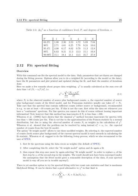
Table 2.4: ∆χ 2 as a function of confidence level, P, and degrees of freedom, ν.
ν
P 1 2 3 4 5 6
68.3% 1.00 2.30 3.53 4.72 5.89 7.04
90% 2.71 4.61 6.25 7.78 9.24 10.6
95.4% 4.00 6.17 8.02 9.70 11.3 12.8
99% 6.63 9.21 11.3 13.3 15.1 16.8
99.99% 15.1 18.4 21.1 13.5 25.7 27.8
2.12 Fit: spectral fitting
Overview
With this command one fits the spectral model to the data. Only parameters that are thawn are changed
during the fitting process. Options allow you to do a weighted fit (according to the model or the data),
have the fit parameters and plot printed and updated during the fit, and limit the number of iterations
done.
Here we make a few remarks about proper data weighting. χ 2 is usually calculated as the sum over all
data bins i of (N i − s i ) 2 /σi 2, i.e. n∑
χ 2 (N i − s i ) 2
= , (2.1)
i=1
where N i is the observed number of source plus background counts, s i the expected number of source
plus background counts of the fitted model, and for Poissonian statistics usually one takes σ 2 i = N i .
Take care that the spectral bins contain sufficient counts (either source or background), recommended
is e.g. to use at least ∼10 counts per bin. If this is not the case, first rebin the data set whenever you
have a ”continuum” spectrum. For line spectra you cannot do this of course without loosing important
information! Note however that this method has inaccuracies if N i is less than ∼100.
Wheaton et al. ([1995]) have shown that the classical χ 2 method becomes inaccurate for spectra with
less than ∼ 100 counts per bin. This is not due to the approximation of the Poisson statistic by a normal
distribution, but due to using the observed number of counts N i as weights in the calculation of χ 2 .
Wheaton et al. showed that the problem can be resolved by using instead σ 2 i = s i , i.e. the expected
number of counts from the best fit model.
The option ”fit weight model” allows to use these modified weights. By selecting it, the expected number
of counts (both source plus background) of the current spectral model is used onwards in calculating the
fit statistic. Wheaton et al. suggest to do the following 3-step process, which we also recommend to the
user of SPEX:
1. first fit the spectrum using the data errors as weights (the default of SPEX).
2. After completing this fit, select the ”fit weight model” option and do again a fit
3. then repeat this step once more by again selecting ”fit weight model” in order to replace s i of the
first step by s i of the second step in the weights. The result should now have been converged (under
the assumption that the fitted model gives a reasonable description of the data, if your spectral
model is way off you are in trouble anyway!).
There is yet another option to try for spectral fitting with low count rate statistics and that is maximum
likelyhood fitting. It can be shown that a good alternative to χ 2 in that limit is
C = 2
σ 2 i
n∑
s i − N i + N i ln(N i /s i ). (2.2)
i=1