SPEX User's Manual - SRON

112 Response matrices
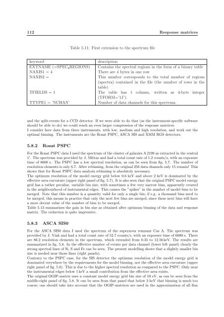
Table 5.11: First extension to the spectrum file
keyword
EXTNAME (=SPEC REGIONS)
NAXIS1 = 4
NAXIS2 =
TFIELDS = 1
TTYPE1 = ’NCHAN’
description
Contains the spectral regions in the form of a binary table
There are 4 bytes in one row
This number corresponds to the total number of regions
(spectra) contained in the file (the number of rows in the
table)
The table has 1 column, written as 4-byte integer
(TFORM=’1J’).
Number of data channels for this spectrum.
and the split-events for a CCD detector. If we were able to do that (as the instrument-specific software
should be able to do) we could reach an even larger compression of the response matrices.
I consider here data from three instruments, with low, medium and high resolution, and work out the
optimal binning. The instruments are the Rosat PSPC, ASCA SIS and XMM RGS detectors.
5.8.2 Rosat PSPC
For the Rosat PSPC data I used the spectrum of the cluster of galaxies A2199 as extracted in the central
1 ′ . The spectrum was provided by J. Mittaz and had a total count rate of 1.2 counts/s, with an exposure
time of 8600 s. The PSPC has a low spectral resolution, as can be seen from fig. 5.7. The number of
resolution elements is only 6.7. After rebinning, from the original 256 data channels only 15 remain! This
shows that for Rosat PSPC data analysis rebinning is absolutely necessary.
The optimum resolution of the model energy grid below 0.6 keV and above 2 keV is dominated by the
effective area curvature (upper right panel of fig. 5.7). It is also seen that the original PSPC model energy
grid has a rather peculiar, variable bin size, with sometimes a few very narrow bins, apparently created
in the neighbourhood of instrumental edges. This causes the ”spikes” in the number of model bins to be
merged. Note that this number is a quantity valid for only a single bin; if e.g. a thousand bins need to
be merged, this means in practice that only the next few bins are merged, since these next bins will have
a more decent value of the number of bins to be merged.
Table 5.13 summarizes the gain in bin size as obtained after optimum binning of the data and response
matrix. The reduction is quite impressive.
5.8.3 ASCA SIS0
For the ASCA SIS0 data I used the spectrum of the supernova remnant Cas A. The spectrum was
provided by J. Vink and had a total count rate of 52.7 counts/s, with an exposure time of 6000 s. There
are 86.2 resolution elements in the spectrum, which extended from 0.35 to 12.56keV. The results are
summarized in fig. 5.8. In the effective number of events per data channel (lower left panel) clearly the
strong spectral lines of Si, S and Fe can be seen. The present modelling shows that a slightly smaller bin
size is needed near those lines (right panels).
Contrary to the PSPC case, for the SIS detector the optimum resolution of the model energy grid is
dominated verywhere by the requirements for the model binning, not the effective area curvature (upper
right panel of fig. 5.8). This is due to the higher spectral resolution as compared to the PSPC. Only near
the instrumental edges below 1 keV a small contribution from the effective area exists.
The original OGIP-matrix uses a constant model energy grid bin size of 10 eV, as can be seen from the
middle-right panel of fig. 5.8. It can be seen from that panel that below 3 keV that binning is much too
coarse; one should take into account that the OGIP-matrices are used in the approximation of all flux