SPEX User's Manual - SRON

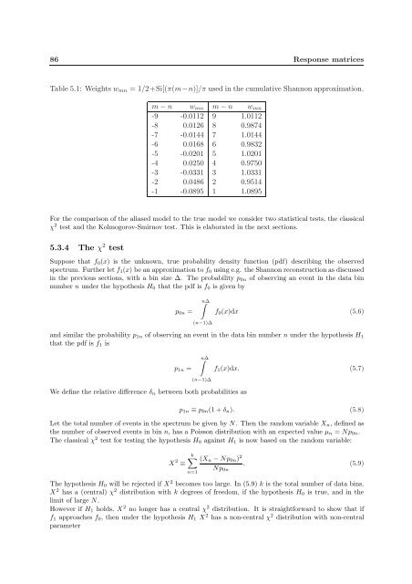
86 Response matrices
Table 5.1: Weights w mn = 1/2+Si[(π(m−n)]/π used in the cumulative Shannon approximation.
m − n w mn m − n w mn
-9 -0.0112 9 1.0112
-8 0.0126 8 0.9874
-7 -0.0144 7 1.0144
-6 0.0168 6 0.9832
-5 -0.0201 5 1.0201
-4 0.0250 4 0.9750
-3 -0.0331 3 1.0331
-2 0.0486 2 0.9514
-1 -0.0895 1 1.0895
For the comparison of the aliased model to the true model we consider two statistical tests, the classical
χ 2 test and the Kolmogorov-Smirnov test. This is elaborated in the next sections.
5.3.4 The χ 2 test
Suppose that f 0 (x) is the unknown, true probability density function (pdf) describing the observed
spectrum. Further let f 1 (x) be an approximation to f 0 using e.g. the Shannon reconstruction as discussed
in the previous sections, with a bin size ∆. The probability p 0n of observing an event in the data bin
number n under the hypothesis H 0 that the pdf is f 0 is given by
p 0n =
∫n∆
(n−1)∆
f 0 (x)dx (5.6)
and similar the probability p 1n of observing an event in the data bin number n under the hypothesis H 1
that the pdf is f 1 is
p 1n =
∫n∆
(n−1)∆
f 1 (x)dx. (5.7)
We define the relative difference δ n between both probabilities as
p 1n ≡ p 0n (1 + δ n ). (5.8)
Let the total number of events in the spectrum be given by N. Then the random variable X n , defined as
the number of observed events in bin n, has a Poisson distribution with an expected value µ n = Np 0n .
The classical χ 2 test for testing the hypothesis H 0 against H 1 is now based on the random variable:
X 2 ≡
k∑ (X n − Np 0n ) 2
n=1
Np 0n
. (5.9)
The hypothesis H 0 will be rejected if X 2 becomes too large. In (5.9) k is the total number of data bins.
X 2 has a (central) χ 2 distribution with k degrees of freedom, if the hypothesis H 0 is true, and in the
limit of large N.
However if H 1 holds, X 2 no longer has a central χ 2 distribution. It is straightforward to show that if
f 1 approaches f 0 , then under the hypothesis H 1 X 2 has a non-central χ 2 distribution with non-central
parameter