SPEX User's Manual - SRON

88 Response matrices
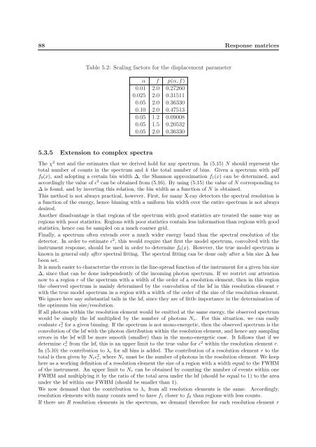
Table 5.2: Scaling factors for the displacement parameter
α f p(α,f)
0.01 2.0 0.27260
0.025 2.0 0.31511
0.05 2.0 0.36330
0.10 2.0 0.47513
0.05 1.2 0.09008
0.05 1.5 0.20532
0.05 2.0 0.36330
5.3.5 Extension to complex spectra
The χ 2 test and the estimates that we derived hold for any spectrum. In (5.15) N should represent the
total number of counts in the spectrum and k the total number of bins. Given a spectrum with pdf
f 0 (x), and adopting a certain bin width ∆, the Shannon approximation f 1 (x) can be determined, and
accordingly the value of ǫ 2 can be obtained from (5.16). By using (5.15) the value of N corresponding to
∆ is found, and by inverting this relation, the bin width as a function of N is obtained.
This method is not always practical, however. First, for many X-ray detectors the spectral resolution is
a function of the energy, hence binning with a uniform bin width over the entire spectrum is not always
desired.
Another disadvantage is that regions of the spectrum with good statistics are treated the same way as
regions with poor statistics. Regions with poor statistics contain less information than regions with good
statistics, hence can be sampled on a much coarser grid.
Finally, a spectrum often extends over a much wider energy band than the spectral resolution of the
detector. In order to estimate ǫ 2 , this would require that first the model spectrum, convolved with the
instrument response, should be used in order to determine f 0 (x). However, the true model spectrum is
known in general only after spectral fitting. The spectral fitting can be done only after a bin size ∆ has
been set.
It is much easier to characterize the errors in the line-spread function of the instrument for a given bin size
∆, since that can be done independently of the incoming photon spectrum. If we restrict our attention
now to a region r of the spectrum with a width of the order of a resolution element, then in this region
the observed spectrum is mainly determined by the convolution of the lsf in this resolution element r
with the true model spectrum in a region with a width of the order of the size of the resolution element.
We ignore here any substantial tails in the lsf, since they are of little importance in the determination of
the optimum bin size/resolution.
If all photons within the resolution element would be emitted at the same energy, the observed spectrum
would be simply the lsf multiplied by the number of photons N r . For this situation, we can easily
evaluate ǫ 2 r for a given binning. If the spectrum is not mono-energetic, then the observed spectrum is the
convolution of the lsf with the photon distribution within the resolution element, and hence any sampling
errors in the lsf will be more smooth (smaller) than in the mono-energetic case. It follows that if we
determine ǫ 2 r from the lsf, this is an upper limit to the true value for ǫ 2 within the resolution element r.
In (5.10) the contribution to λ c for all bins is added. The contribution of a resolution element r to the
total is then given by N r ǫ 2 r , where N r must be the number of photons in the resolution element. We keep
here as a working definition of a resolution element the size of a region with a width equal to the FWHM
of the instrument. An upper limit to N r can be obtained by counting the number of events within one
FWHM and multiplying it by the ratio of the total area under the lsf (should be equal to 1) to the area
under the lsf within one FWHM (should be smaller than 1).
We now demand that the contribution to λ c from all resolution elements is the same. Accordingly,
resolution elements with many counts need to have f 1 closer to f 0 than regions with less counts.
If there are R resolution elements in the spectrum, we demand therefore for each resolution element r