SPEX User's Manual - SRON

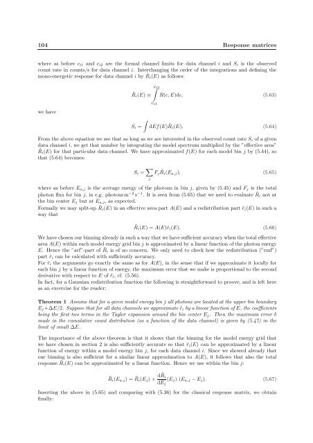
104 Response matrices
where as before c i1 and c i2 are the formal channel limits for data channel i and S i is the observed
count rate in counts/s for data channel i. Interchanging the order of the integrations and defining the
mono-energetic response for data channel i by ˜R i (E) as follows:
we have
∫c i2
˜R i (E) ≡ R(c, E)dc, (5.63)
c i1
∫
S i = dEf(E) ˜R i (E). (5.64)
From the above equation we see that as long as we are interested in the observed count rate S i of a given
data channel i, we get that number by integrating the model spectrum multiplied by the ”effective area”
˜R i (E) for that particular data channel. We have approximated f(E) for each model bin j by (5.44), so
that (5.64) becomes:
S i = ∑ j
F j ˜Ri (E a,j ), (5.65)
where as before E a,j is the average energy of the photons in bin j, given by (5.45) and F j is the total
photon flux for bin j, in e.g. photonsm −2 s −1 . It is seen from (5.65) that we need to evaluate ˜R i not at
the bin center E j but at E a,j , as expected.
Formally we may split-up ˜R i (E) in an effective area part A(E) and a redistribution part ˜r i (E) in such a
way that
˜R i (E) = A(E)˜r i (E). (5.66)
We have chosen our binning already in such a way that we have sufficient accuracy when the total effective
area A(E) within each model energy grid bin j is approximated by a linear function of the photon energy
E. Hence the ”arf”-part of ˜R i is of no concern. We only need to check how the redistribution (”rmf”)
part ˜r i can be calculated with sufficiently accuracy.
For ˜r i the arguments go exactly the same as for A(E), in the sense that if we approximate it locally for
each bin j by a linear function of energy, the maximum error that we make is proportional to the second
derivative with respect to E of ˜r i , cf. (5.56).
In fact, for a Gaussian redistribution function the following is straightforward to proove, and is left here
as an excercise for the reader:
Theorem 1 Assume that for a given model energy bin j all photons are located at the upper bin boundary
E j +∆E/2. Suppose that for all data channels we approximate ˜r i by a linear function of E, the coefficients
being the first two terms in the Taylor expansion around the bin center E j . Then the maximum error δ
made in the cumulative count distribution (as a function of the data channel) is given by (5.47) in the
limit of small ∆E.
The importance of the above theorem is that it shows that the binning for the model energy grid that
we have chosen in section 2 is also sufficiently accurate so that ˜r i (E) can be approximated by a linear
function of energy within a model energy bin j, for each data channel i. Since we showed already that
our binning is also sufficient for a similar linear approximation to A(E), it follows that also the total
response ˜R i (E) can be approximated by a linear function. Hence we use within the bin j:
˜R i (E a,j ) = ˜R i (E j ) + d ˜R i
dE j
(E j ) (E a,j − E j ). (5.67)
Inserting the above in (5.65) and comparing with (5.36) for the classical response matrix, we obtain
finally: