SPEX User's Manual - SRON

5.3 Data binning 91
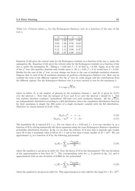
Table 5.5: Critical valuse c α for the Kolmogorov-Smirnov test as a function of the size of the
test α
α c α α c α
0.01 1.63 0.27 1.00
0.05 1.36 0.50 0.83
0.10 1.22 0.95 0.52
0.15 1.14 0.98 0.47
0.20 1.07 0.99 0.44
Equation (5.23) gives the critical value for the Kolmogorov-statistic as a function of the size α, under the
assumption H 0 . Equation (5.24) gives the critical value for the Kolmogorov-statistic as a function of the
size α, under the assumption H 1 . Taking α = 0.05 and f = 2, we find λ k = 0.134. Again, as in the case
of the χ 2 test, this quantity depends only weakly upon α: for α = 0.01, f = 2 we would have λ = 0.110.
Similar for the case of the χ 2 test, we now change our focus to the case of multiple resolution elements.
Suppose that in each of the R resolution elements we perform a Kolmogorov-Smirnov test. How can we
combine the tests in the different regions? For the χ 2 test we could simply add the contributions from
the different regions. For the Kolmogorov-Smirnov test it is more natural to test for the maximum δ:
√
δ ≡ max Nr D r , (5.25)
r
where as before N r is the number of photons in the resolution element r, and D r is given by (5.21)
over the interval r. Note that the integral of S r (x) and F r (x) over the interval r should be 1. Our
test statistic therefore combines ”normalized” KS-tests over each resolution element. All the √ N r D r
are independently distributed according to a KS distribution, hence the cumulative distribution function
for their maximum is simply the Rth power of a single stochastic variable with the KS distribution.
Therefore we obtain instead of (5.23, 5.24):
F KS (c α ) R = 1 − α, (5.26)
F KS (c α − λ k ) R = 1 − fα. (5.27)
The hypothesis H 0 is rejected if δ > c α . For our choice of α = 0.05 and f = 2 we can calculate λ k as a
function of R by solving numerically the above equations using the exact Kolmogorov-Smirnov cumulative
probability distribution function. In fig. 5.1 we show the solution. It is seen that it depends only weakly
upon R; it has a maximum value 0.134 at R = 1 and is less than 3 times smaller at R = 10 10 . We can
approximate λ k as a function of R by the following polynomial:
λ k (R) =
5∑ 10 log(R)
a i ( ) i , (5.28)
10
i=0
where the numbers a i are given in table 5.6. Note the factor of 10 in the denominator! The rms deviation
of the approximation is less then 10 −4 . The corresponding value for c α is plotted in fig. 5.2, and is
approximated with an rms deviation of 0.0004 by the polynomial:
c α (R) =
5∑ 10 log(R)
b i ( ) i , (5.29)
10
i=0
where the numbers b i are given in table 5.6. This approximation is only valid for the range 0.5 < R < 10 10 .