shooting method for nonlinear singularly perturbed boundary-value ...

SHOOTING METHOD FOR NONLINEAR SINGULARLY
PERTURBED BOUNDARY-VALUE PROBLEMS
by
C. H. Ou ∗ and R. Wong ∗
Abstract
Asymptotic formulas, as ε → 0 + , are derived for the solutions of the nonlinear differential
equation εu ′′ +Q(u) = 0 with boundary conditions u(−1) = u(1) = 0 or u ′ (−1) =
u ′ (1) = 0. The nonlinear term Q(u) behaves like a cubic; it vanishes at s − , 0, s + and
nowhere else in [s − , s + ], where s − < 0 < s + . Furthermore, Q ′ (s ± ) < 0, Q ′ (0) > 0 and
the integral of Q on the interval [s − , s + ] is zero. Solutions to these boundary-value problems
are shown to exhibit internal shock layers, and the error terms in the asymptotic
approximations are demonstrated to be exponentially small. Estimates are obtained
for the number of internal shocks that a solution can have, and the total numbers of
solutions to these problems are also given. All results here are established rigorously in
the mathematical sense.
∗ Department of Mathematics, City University of Hong Kong, Tat Chee Avenue, Kowloon,
Hong Kong.

1 INTRODUCTION
In this paper, we consider the singularly perturbed two-point problem
(1.1) εu ′′ + Q(u) = 0, −1 < x < 1,
with boundary conditions
(1.2) u(−1) = u(1) = 0
or
(1.3) u ′ (−1) = u ′ (1) = 0,
where ε is a small positive parameter. Throughout the paper, we shall assume that the
nonlinear term Q(u) vanishes at s − , 0, s + and nowhere else in [s − , s + ], where s − < 0 < s + .
Furthermore, we assume that Q ′ (s ± ) < 0, Q ′ (0) > 0 and
(1.4)
∫ s+
s −
Q(s)ds = 0.
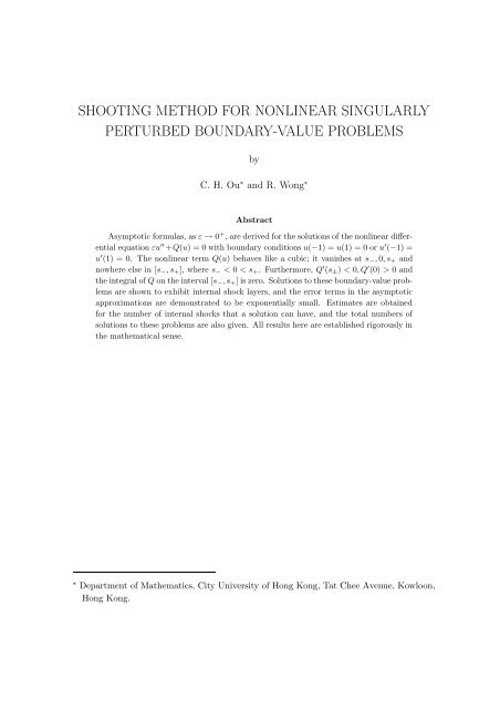
The graph of the function Q(u) has the typical shape shown in Figure 1.
Equation (1.1) can be considered as the equation of motion of a nonlinear spring with
spring constant large compared to the mass. It is also the equilibrium equation associated
with the Ginzburg-Landau model
(1.5) u t = εu xx + Q(u), −1 < x < 1, t ≥ 0,
with various boundary conditions at x = ±1. In (1.5), Q(u) = −Ṽ ′ (u), where Ṽ (u) is a
double well potential with wells of equal depth located at the preferred phases u = s − and
u = s + .
Q(u)
s
- +
s
u
Figure 1. Graph of Q(u).
The problem of finding asymptotic behavior of the solutions to (1.1) & (1.2) or (1.1)
& (1.3) has been studied earlier by O’Malley [5], using a phase-plane analysis. Although
2

his approach provides useful qualitative information about the solutions with internal layer
behavior, it does not give quantitative information such as asymptotic formulas for the
solutions. The best known approach to derive such formulas is probably the method of
matched asymptotics. But, as was shown by Carrier and Pearson [1, p.202], a routine
application of this method will not lead to the determination of the locations of the internal
layers, thus creating spurious solutions. To overcome this difficulty, Lange [3] extended the
method of matched asymptotics by including exponentially small terms in the expansion
of the solution; see also MacGillivray [4]. There are two difficulties with Lange’s approach;
namely, (i) explicit expressions for the internal layer solutions must be known a priorily, (ii)
second-order terms in the asymptotic expansions are needed to determine the layer positions
of the leading order approximate solutions. An alternative approach has been introduced
by Ward [8], which he later called the projection method (see [7, p.496]). Ward’s method
is an extension of the variational approach adopted by Kath et al [2], and does not require
the knowledge of the explicit form of the internal layer solution. However, as stated by
himself in [8, p.98], he is not able to determine the number of solutions to (1.1) for small
fixed ε. More recently, Reyna and Ward [7] introduced another method, which involves
a nonlinear WKB-type transformation for (1.1). The advantage of this method is that it
avoids the use of exponential asymptotics, i.e., it is sufficient to use just the conventional
singular perturbation approach on the transformed problem.
Despite the usefulness of all these methods mentioned above in providing approximate
solutions to the problem (1.1) & (1.2) or (1.1) & (1.3) they have a common defect from
a mathematical point of view; that is, none of the arguments used in these methods can
be modified to show that for each approximate solution, there is one and only one true
solution, and that their difference in absolute value tends to zero as ε approaches zero. A
first attempt in this direction was made in [6], where only the special case Q(u) = 1−u 2 was
considered. For instance, it was shown in [6] that in this special case, there exists exactly
one solution u 1 (x, ε) to (1.1) & (1.2) satisfying
( ) x√ε
(1.6) u 1 (x, ε) = ũ 1 (x, ε) + q + O(e −√2/ε ),
where
(1.7)
( x + 1
ũ 1 (x, ε) = −1 + 3sech 2 √ + ln( √ 3 + √ )
2)
2ε
( 1 − x
+ 3sech 2 √ + ln( √ 3 + √ )
2)
2ε
and
(1.8) q(ζ) = 12e√ 2ζ
(1 + e √ 2ζ ) 2 .
The graph of the solution u 1 (x, ε) is shown in Figure 2.
3

2
_
1 1
0
_
1
Figure 2. Graph of the solution u 1 (x, ε) when ε = 0.01
The internal layer near the origin is called a spike. Furthermore, it was shown in [6]
that if n(ε) denotes the number of solutions to the boundary-value problem (BVP) − (1.1)
& (1.2) when Q(u) = 1 − u 2 , then we have the asymptotic formula
(1.9) n(ε) ∼ 1.64 √ ε
as ε → 0 + .
As to the maximum number, say N(ε), of spikes that a solution to (1.1) & (1.2) can have,
we have the estimate
(1.10) N(ε) ≤ 0.41 √ ε
+ 1.
In the present paper, we shall establish corresponding results for the BVP (1.1) & (1.2)
or (1.1) & (1.3), when Q(u) is of the form shown in Figure 1. For instance, in the case when
Q(u) = 2u − 2u 3 which was considered by Lange [3], we will show that there exist exactly
two solutions u 1,1 (x, ε) and u 1,2 (x, ε) to (1.1) & (1.2) such that
(1.11) u 1,2 (x, ε) = u 1,1 (−x, ε)
and
(1.12)
( ) x + 1
u 1,1 (x, ε) = tanh √ + tanh
(− x )
√ ε ε
( ) x − 1
+ tanh √ + O(e −1/√ε ).
ε
The graph of u 1,1 (x, ε) is shown in Figure 3. The internal layer near x = 0 in this case is
called a shock. An estimate for the maximum number n 1 (ε) of shocks is given by
4

1
_
1
1
_
1
Figure 3. Graph of u 1,1 (x, ε) when ε = 0.01.
(1.13) n 1 (ε) ≤ 2 π
√
2
ε − 1,
and the number n 2 (ε) of solutions to (1.1) – (1.2) behaves like
(1.14) n 2 (ε) ∼ 4 π
√
2
ε .
The presentation of this paper is arranged as follows. In §2, we consider an initialvalue
problem (IVP), which is directly related to the BVP (1.1) – (1.2). We show that the
existence of a solution to (1.1) – (1.2) depends very much on the slope of the solution to
this IVP at x = −1. We also establish some properties about the lengths of the intervals in
which the solution to this IVP is above or below the x-axis. In addition, we give estimates
for the number of solutions to (1.1) – (1.2), and the maximum number of shocks that a
solution can have. In §3, we examine the asymptotic nature of the approximate solutions
in the case when there is no shocks or at most one shock. In fact, we shall prove that
the differences between approximate solutions and true solutions are exponentially small.
The results for the general case with n shocks are presented in §4. In §5, we state the
corresponding results for the BVP (1.1) & (1.3). Two special but typical examples are
given in §6. The final section contains discussions of some cases not touched upon in the
previous sections, including the boundary-value problem consisting of equation (1.1) and
the boundary conditions
(1.15)
√ εu ′ (1) + k r (u(1) − s + ) = 0
and
(1.16)
√ εu ′ (−1) − k l (u(−1) − s − ) = 0
studied in Ward [8].
5

2 NUMBER OF SHOCKS
As in our previous paper [6], our approach is based on the shooting method. That is,
we start with the initial-value problem (IVP)
(2.1)
{
εu ′′ + Q(u) = 0
u(−1) = 0, u ′ (−1) = k,
where k is a real number. When Q(u) is sufficiently smooth, it is known that this problem
has a unique solution which can be extended to all x > −1. For convenience, we introduce
the notation
√
∫
2 s+
(2.2) k max := Q(s) ds.
ε 0
LEMMA 1. Let u(x, k) denote the solution to the IVP (1.1) − (1.2). If k > k max ,
then u(x, k) is increasing for x > −1 and lim x→∞ u(x, k) = ∞. (b) If k < −k max , then
u(x, k) is decreasing for x > −1 and lim x→∞ u(x, k) = −∞. (c) If |k| < k max , then u(x, k)
is periodic and intersects the x-axis infinitely many times. (d) In the critical case, i.e. when
k = ±k max , u(x, ε) = ±f(ξ) where ξ = x+1 √ ε
and f satisfies
(2.3) f ′′ (ξ) + Q(f) = 0, −∞ < ξ < ∞,
(2.4) f(−∞) = s − , f(∞) = s + , f(0) = 0;
furthermore,
(2.5) f(ξ) ∼ s + − A + e −σ +ξ , as ξ → ∞
and
(2.6) f(ξ) ∼ s − + A − e σ −ξ , as ξ → −∞,
where σ ± = (−Q ′ (s ± )) 1/2 , and A + , A − are explicitly given positive constants.
Proof. (a) Multiplying both sides of the differential equation in (2.1) by u ′ , and integrating
from −1 to x, we obtain
(2.7)
ε
2 (u′ ) 2 +
∫ u
0
Q(s)ds = C,
where C = ε 2 k2 . If k > k max , then it is easily seen from the graph of Q(s) that C > ∫ u
0 Q(s)ds
for any u > 0 and ε 2 (u′ ) 2 > 0; cf. (2.2). Since u ′ (−1, ε) = k > 0 and u ′ (x, ε) never vanishes,
it follows that u ′ (x, ε) > 0 for x > −1. Therefore, u(x, ε) is increasing for x > −1 and we
can assume that
lim u(x, ε) = l.
x→∞
6

We shall show that l = ∞. Since k > k max , there is a number β > 0 such that
k 2 > 2 ε
∫ s+
Substituting this inequality into (2.7) gives
for x > −1, from which it follows that
0
u ′ (x) > √ β
Q(s)ds + β.
lim u(x, ε) = ∞.
x→∞
(b) The argument in this case is similar to that in case (a). Using (2.7), one can easily
show that u(x, ε) is decreasing for x > −1, and that it tends to −∞ as x approaches ∞.
(c) We consider only the case 0 < k < k max ; the argument for −k max < k < 0 is more
or less the same. From the graph of Q(u) in Figure 1, it is readily seen that the equation
∫ u
0 Q(s)ds = C has two roots u 1(k) and u 2 (k) such that u 1 (k) ∈ (0, s + ) and u 2 (k) ∈ (s − , 0).
From the initial conditions in (2.1) and equation (2.7), it also follows that there are two
points x = d 1 and x = d 2 with d 1 < d 2 such that
u ′ (d 1 , k) = 0, u(d 1 , k) = u 1 (k) ∈ (0, s + ),
and
u(d 2 , k) = 0,
u ′ (d 2 , k) = −k.
Starting from x = d 2 , one can also show that there exist two points d 3 and d 4 such that
u ′ (d 3 , k) = 0, u(d 3 , k) = u 2 (k) ∈ (s − , 0),
and
u(d 4 , k) = 0, u ′ (d 4 , k) = k.
At x = d 4 , u(x, k) has the same initial values as those at the starting point x = −1. Hence,
u(x, k) is periodic with period d 4 + 1.
In the case k = 0, u ≡ 0 is the only solution to (2.1).
(d) When |k| = k max , we have C = ε 2 k2 = ∫ s +
0
Q(s)ds. First, consider the case k = k max ,
and make the change of variables
(2.8) ξ = x + 1 √ ε
,
f(ξ) = u(x, k).
It is readily verified that f satisfies (2.3). From (2.7), it also follows that
(2.9)
We claim
( )
1 df 2 ∫ f ∫ s+
+ Q(s)ds = Q(s)ds.
2 dξ 0
0
(2.10) 0 < f < s +
7

for ξ > 0 and
(2.11) lim
ξ→∞
f(ξ) = s + .
Since f(0) = u(−1, k) = 0, it is easily seen that f(ξ) < s + for ξ in a right neighborhood
of 0. From (2.9), it can also be seen that there is such a neighborhood in which f ′ (ξ) > 0,
i.e., f(ξ) is increasing. We shall show that in fact, f(ξ) is increasing in the whole interval
0 < ξ < ∞. Assume to the contrary that there exists a point η such that f(η) = s + and
0 < f(ξ) < s + for 0 < ξ < η. Put
(2.12) V (f) :=
∫ f
s +
Q(s)ds.
Clearly, V (s + ) = V ′ (s + ) = 0 and V ′′ (s + ) = Q ′ (s + ) < 0. Since V (f) is sufficiently smooth,
we may write V (f) = (s + − f) 2 H(f), where H(f) is a negative function, so that
(2.13) σ + = √ −Q ′ (s + ) = √ −2H(s + ).
(Note that as long as ξ < η, we have f < s + and V < 0.) From (2.9), we obtain
(2.14)
df
(s + − f) √ −2H(f) = dξ.
Integrating both sides from ξ = 0 to ξ = η gives
(2.15)
∫ s+
0
∫
df
η
(s + − f) √ −2H(f) =
which is not possible since the left-hand side is infinite while the right-hand is finite; this
completes the proof of (2.10). Since f ′ (ξ) is positive in a right neighborhood of the origin
and does not vanish elsewhere, it follows from (2.9) that f ′ (ξ) > 0, i.e., f(ξ) is increasing,
in 0 < ξ < ∞ and
lim
ξ→∞ f(ξ) = l ≤ s +.
To show that l = s + , we integrate (2.14) on both sides form 0 to ∞ to yield
∫ l
0
df
(s + − f) √ −2H(f) = ∞,
from which it follows that l = s + , thus proving (2.11).
To derive the asymptotic behavior of f(ξ), we return to (2.14) and obtain
(2.16)
0
∫ f
0
ds
(s + − s) √ −2H(s) = ξ.
The integral on the left-hand side can be written as
∫ f
∫
ds
s+
(
(s + − s) √ −2H(s + ) + 1 1
√ √ −
2(s+ − s) −H(s)
−
0
∫ s+
f
1
√
2(s+ − s)
8
0
dξ,
(
1
√ −
−H(s)
)
1
√ ds
−H(s+ )
)
1
√ ds.
−H(s+ )

On account of (2.13), this gives
(2.17)
∫ f
0
ds
(s + − s) √ −2H(s) = 1 [ln(s + ) − ln(s + − f)] + c + − c 2 (f),
σ +
where
(2.18) c + =
and
(2.19) c 2 (f) =
∫ s+
f
∫ s+
0
(
)
1
1
√ −
ds
−2V (s) (s + − s)σ +
(
1
√
2(s+ − s)
1
√ −
−H(s)
)
1
√ ds.
−H(s+ )
Note that the last two integrals are well defined. Coupling (2.16) and (2.17), we have
f = s + − s + e σ +c +
e −σ +ξ e −c 2(f)σ +
.
Since c 2 (f) → 0 as f → s + , the result in (2.5) follows with A + = s + e σ +c +
.
argument can be used to demonstrate (2.6) with A − = −s − e σ −c −
where
∫ s−
(
)
−1
1
c − = √ −
ds
−2V (s) (s − − s)σ −
0
A similar
This completes the proof of the lemma.
REMARK 1. The proof of case (d) above actually gives the existence of a monotonically
increasing function f(ξ), which satisfies the differential equation in (2.3) and the
conditions in (2.4). Furthermore, it has the asymptotic behavior given in (2.5) and (2.6).
This result is stated explicitly in Ward [8, p.99], but without a proof.
REMARK 2. Using (2.13) and (2.14), one can also deduce from (2.5) and (2.6)
(2.20) f ′ (ξ) ∼ σ + A + e −σ +ξ , as ξ → ∞,
(2.21) f ′ (ξ) ∼ σ − A − e σ −ξ , as ξ → −∞.
From Lemma 1, it is clear that in order to have u(1, k) = 0, we must choose k in the
interval (−k max , 0) or (0, k max ), in which case the solution to the initial-value problem (2.1)
is periodic and intersects the x-axis infinitely many times.
We consider only the case k ∈ (0, k max ), since the case k ∈ (−k max , 0) is entirely similar.
Let x 1 be the first point to the right of −1 such that u(x 1 , k) = 0 and u(x, k) > 0 for
−1 < x < x 1 , and x 2 be the first point to the right of x 1 such that u(x 2 , k) = 0 and
u(x, k) < 0 for x 1 < x < x 2 . We denote by T 1 (k) and T 2 (k), respectively, the lengths of the
interval [−1, x 1 ] and [x 1 , x 2 ]. From (2.7) and the graph of Q(u) in Figure 1, we can also
find two points u 1 (k) ∈ (0, s + ) and u 2 (k) ∈ (s − , 0) such that
∫ 0
(2.22) − Q(s)ds =
u 2 (k)
∫ u1 (k)
0
9
Q(s)ds = ε 2 k2 .

It is readily seen that when k → 0, u 1 (k) and u 2 (k) tend to zero and when k → k max , u 1 (k)
tends to s + and u 2 (k) tends to s − . Differentiating both sides of (2.22) with respect to k
shows that u ′ 1 (k) > 0 and u′ 2 (k) < 0. From (2.7), we obtain
(2.23)
from which it follows that
√ du ε √
2 ∫ u 1 (k)
u
Q(s)ds
= dx,
(2.24) T 1 (k) = √ 2ε
and
(2.25) T 2 (k) = √ 2ε
∫ u1 (k)
0
∫ 0
u 2 (k)
du
√ ∫ u1 (k)
Q(s)ds
u
du
√ ∫
.
u2 (k)
Q(s)ds
In the case k ∈ (−k max , 0), the solution u(x, k) to the initial-value problem (2.1) is again
oscillatory about the x-axis, except that it now starts at x = −1 with a negative slope.
Hence, the graph of u(x, k) is below the x-axis in the interval (−1, x 1 ), where x 1 is the
first point to the right of −1 at which u(x, k) meets the line u = 0 again, i.e., u(x, k) < 0
in (−1, x 1 ). Let x 2 denote the first point to the right of x 1 such that u(x 2 , k) = 0 and
u(x, k) > 0 for x 1 < x < x 2 . Unlike before, we now reverse the order, and denote by T 2 (k)
and T 1 (k) the length of the intervals [−1, x 1 ] and [x 1 , x 2 ], respectively. Hence, the values of
T 1 (k) and T 2 (k) are actually dependent on the value of |k|.
LEMMA 2. We have
Proof. Let
lim
k→0 + T 1(k) = lim
k→0 + T 2(k) =
V 2 (u) =
∫ u
0
u
Q(s)ds.
π√ ε
√
Q ′ (0) .
Since V 2 (u) is sufficiently smooth and V 2 (0) = V ′
2 (0) = 0, we may write V 2(u) = u 2 G(u),
where G is a sufficiently smooth function with G(0) = 1 2 Q′ (0). From (2.24), it follows that
(2.26)
T 1 (k) = √ ∫ u1 (k)
du
2ε √
V2 (u 1 (k)) − V 2 (u)
= √ 2ε
0
∫ u1 (k)
0
du
√
u
2
1 (k)G(u 1 (k)) − u 2 G(u) .
It is easily seen that
√
2ε
∫ u1 (k)
0
du
√
G(0)(u
2
1 (k) − u 2 ) = π 2
√
2ε
√
G(0)
=
π√ ε
√
Q ′ (0) .
10

Since the integral
√
∫ u1 (k)(
)
1
2ε √
V2 (u 1 (k)) − V 2 (u) − 1
√ du.
G(0)(u
2
1 (k) − u 2 )
0
exists and the length of the integration interval tends to zero as k → 0, we obtain
T 1 (k) −
π√ ε
√ → 0 as k → 0.
Q ′ (0)
In a similar manner, one can prove
lim T 2(k) =
k→0 +
π√ ε
√
Q ′ (0) .
On the other hand, we have u 1 (k) → s + and u 2 (k) → s − as k → k max ; see the second
paragraph following Remark 2. Hence
(2.27) lim T 1 (k) = lim T 2 (k) = ∞.
k→k max k→k max
Put
(2.28) t 1 := inf
0

that the number of zeros, which corresponds to the number of shocks, of a solution u(x, k)
in the interval (−1, 1) is N + M − 1. Therefore, the number of shock layers is N + M − 1.
From here on, our task is to choose appropriate values of k, and determine possible
integers N and M, so that (2.32) holds.
For ε > 0, we define
[ ]
2
(2.33) N 1 (ε) :=
t 1 + t 2
and
[
(2.34) N 2 (ε) :=
2
T 1 (0 + ) + T 2 (0 + )
where t 1 , t 2 are given above and [x] denotes the largest integer less than or equal to x.
The following result provides estimates for the number of shocks that the solutions to BVP
(1.1)–(1.2) can have.
LEMMA 3. If N ≥ N 1 (ε) + 1 and M ≥ N 1 (ε) + 1, then there exists no slope k such
that (2.32) holds, i.e., the BVP (1.1) − (1.2) has no solution with more than or equal to
2N 1 (ε) + 1 shocks. If N ≤ N 2 (ε) and M ≤ N 2 (ε), then there exists at least one value of k
so that (2.32) holds, i.e., BVP (1.1) − (1.2) has at least one solution with N + M − 1 shocks.
Proof. The function
NT 1 (k) + MT 2 (k)
is continuous in 0 < k < k max . For any k > 0, we have by (2.33)
NT 1 (k) + MT 2 (k) ≥ Nt 1 + Mt 2
]
,
≥ (N 1 (ε) + 1)t 1 + (N 1 (ε) + 1)t 2
= (N 1 (ε) + 1)(t 1 + t 2 ) > 2.
Thus, (2.32) fails to hold and the boundary-value problem has no solution.
If N ≤ N 2 (ε) and M ≤ N 2 (ε), then by (2.34) and (2.27) the function NT 1 (k) + MT 2 (k)
satisfies
lim
k→0 +
NT 1 (k) + MT 2 (k) ≤ N 2 (ε)(T 1 (0 + ) + T 2 (0 + )) ≤ 2
and
lim
k→k max
NT 1 (k) + MT 2 (k) = ∞.
In view of the continuity of the function NT 1 (k) + MT 2 (k), there exists at least one point
k 0 ∈ (0, k max ) such that
NT 1 (k 0 ) + MT 2 (k 0 ) = 2,
which means that there exists at least one solution to BVP (1.1)-(1.2). Also, it follows that
this solution has N +M −1 zeros, and hence N +M −1 internal shock layers, in the interval
(−1, 1).
When Q(u) satisfies the additional condition given below, we can in fact establish the
monotonicity of T 1 (k) and T 2 (k) with respect to k, in which case more accurate estimates
for the numbers of shocks and solutions can be obtained.
12

LEMMA 4. If, in addition, Q(s)/s is decreasing in s for s ∈ (0, s + ) and increasing
for s ∈ (s − , 0), then T 1 (k) and T 2 (k) are increasing in k for k ∈ (0, k max ).
Proof. From (2.24), we have
T 1 (k) = √ 2ε
Changing variables u = u 1 (k)t yields
where
Straightforward differentiation gives
df 1
= 1 (
du 1 u 3 Q(u 1 )u 1 − 2
1
∫ u1 (k)
0
T 1 (k) = √ 2ε
du
√ ∫
.
u1 (k)
Q(s)ds
∫ 1
0
u
dt
√
f1 (k) ,
f 1 (k) = 1 ∫ u1 (k)
u 2 1 (k) Q(s)ds.
∫ u1
0
u 1 (k)t
∫ tu1
)
Q(s)ds − [Q(tu 1 )tu 1 − 2 Q(s)ds] .
0
Since Q(x)/x is decreasing, we have Q ′ (x)x − Q(x) < 0 for almost all x ∈ (0, s + ), from
which it follows that Q(x)x − 2 ∫ x
0
Q(s)ds is decreasing. Hence
df 1
du 1
< 0
and
df 1
dk = df 1
du 1
du 1
dk < 0
for almost all k ∈ (0, k max ); see a statement following (2.22). Note that dT 1 /df 1 is negative.
Thus, by the chain rule,
dT 1 (k)
> 0,
dk
i.e., T 1 (k) is increasing in k. The proof of the monotonicity of T 2 (k) is similar; this completes
the proof of the lemma.
From Lemma 4, it follows that
(2.35) t 1 = t 2 = T 1 (0 + ) = T 2 (0 + ) = π√ ε
√
Q ′ (0) .
REMARK 3. Note that the function sQ ′ (s) − Q(s) vanishes at s = 0, is negative
in (0, s + ) and positive in (s − , 0). Hence, if Q(s) satisfies Q ′′ (s) < 0 for s ∈ (0, s + ) and
Q ′′ (s) > 0 for s ∈ (0, s − ), then the condition in Lemma 4 holds and T 1 (k), T 2 (k) are increasing
in k for 0 < k < k max .
Let
[ ] [ √
2 2 Q
(2.36) N(ε) = =
′ ]
(0)
t 1 π √ .
ε
We have the following result concerning the numbers of shocks and solutions to the BVP
(1.1) − (1.2)
13

THEOREM 1. Let n 1 (ε) denote the numbers of shocks that a solution to (1.1)−(1.2)
can have, and let n 2 (ε) denote the number of solutions to (1.1)−(1.2). If Q(s)/s is decreasing
for s ∈ (0, s + ) and increasing for s ∈ (s − , 0), then n 1 (ε) satisfies
0 ≤ n 1 (ε) ≤ N(ε) − 1,
and n 2 (ε) satisfies
n 2 (ε) = 2N(ε),
where N(ε) is given in (2.36).
Proof. If n 1 (ε) ≤ N(ε) − 1, we choose
[ ]
n1 (ε) + 1
(2.37) M =
2
and
[ ]
n1 (ε) + 1
(2.38) N = n 1 (ε) −
+ 1.
2
Then N ≥ M, N + M = n 1 (ε) + 1 ≤ N(ε), and
N − M ≤ 1.
Consider the function
NT 1 (k) + MT 2 (k).
By (2.35) and (2.36), we have
and
lim
k→0 +
NT 1 (k) + MT 2 (k) = (N + M)t 1
= (n 1 (ε) + 1)t 1 ≤ N(ε)t 1 ≤ 2
lim
k→k max
NT 1 (k) + MT 2 (k) = ∞.
Since by Lemma 4 this function is increasing in k, there exists a unique point k 0 such that
NT 1 (k 0 ) + MT 2 (k 0 ) = 2.
If n 1 (ε) ≥ N(ε), then N + M ≥ n 1 (ε) + 1 ≥ N(ε) + 1 and by (2.28) and (2.36)
NT 1 (k) + MT 2 (k) ≥ (N + M)t 1 ≥ (N(ε) + 1)t 1 > 2
for any k. Thus, we cannot expect (2.32) to hold, i.e., there exists no solution to problem
(1.1) − (1.2) if n 1 (ε) ≥ N(ε).
On one hand, for any n 1 (ε) in 0 ≤ n 1 (ε) ≤ N(ε) − 1, we can choose M and N as
given in (2.37) and (2.38) so that there exists exactly one value k 0 satisfying u(1, k 0 ) = 0.
On the other hand, by interchanging the two values of M and N in (2.37) and (2.38) and
14

considering k ∈ (−k max , 0), we conclude by the symmetry that u(1, −k 0 ) = 0. Therefore,
there are exactly two solutions with n 1 (ε) shock layers.
Adding all solutions together, we get the number of solutions to (1.1) − (1.2) given by
This completes the proof of the theorem.
n 2 (ε) = 2N(ε).
When Q(u) = 2u − 2u 3 , Q(u)/u = 2 − 2u 2 is decreasing for u > 0 and increasing for
u < 0. Therefore, Lemma 4 applies and both T 1 (k) and T 2 (k) are increasing in k for k > 0.
For k < 0, the situation is just the opposite and both T 1 (k) and T 2 (k) are decreasing in k
for k < 0. In fact, T 1 (k) and T 2 (k) depend on the absolute value of k (i.e., |k|), and we have
T 1 (k) = T 1 (−k),
T 2 (k) = T 2 (−k).
From (2.35) and (2.36), it follows that
t 1 = inf
k>0 T 1(k) = T 1 (0 + ) =
√ επ
√
2
and
[ ] 2
N(ε) = =
t 1
[ 2
√
2
√ επ
].
Applying Theorem 1, we obtain the following result.
COROLLARY 1. If Q(u) = 2u − 2u 3 , then the number n 1 (ε) of shocks, that a
solution to problem (1.1) − (1.2) can have, satisfies
[ √ ] 2 2
0 ≤ n 1 (ε) ≤ N(ε) − 1 = √ − 1. επ
Moreover, the number n 2 (ε) of solutions to (1.1) − (1.2) satisfies
n 2 (ε) = 2N(ε) = 2[ 2√ 2
√ επ
] ∼ 4√ 2
√ επ
.
If Q(u) = sin(πu), then s(Q(s)/s) ′ ≤ 0 for s ∈ [−1, 1], Q ′ (0) = π and N(ε) = [ 2
√ πε
]
. A
similar result is obtained.
COROLLARY 2. If Q(u) = sin(πu), then the number n 1 (ε) of shocks, that a solution
to problem (1.1) − (1.2) can have, satisfies
[ ] 2
0 ≤ n 1 (ε) ≤ N(ε) − 1 = √ − 1. πε
Moreover, the number n 2 (ε) of solutions to (1.1) − (1.2) satisfies
[ ] 2
n 2 (ε) = 2N(ε) = 2 √ ∼ √ 4 .
πε επ
15

3 APPROXIMATE SOLUTIONS WITH AT MOST ONE
SHOCK
First, we confine ourselves to solutions with no shock layers, i.e., solutions which is either
entirely positive, or entirely negative, in the interval (−1, 1).
THEOREM 2. The BVP problem (1.1)−(1.2) has one and only one solution u 0,1 (x)
which is positive in the interval (−1, 1). The asymptotic formula for this solution is given
by
( ) ( ) ( )
x + 1 1 − x
(3.1) u 0,1 (x) = f √ + f √ − s + + O e −σ +/ √ ε
,
ε ε
where f is the function given in Lemma 1(d). Likewise, the problem (1.1) − (1.2) also has
one and only one solution u 0,2 (x) which is negative in the interval (−1, 1). The asymptotic
formula for this solution is given by
(3.2) u 0,2 (x) = f
(
− x + 1 √ ε
)
+ f
(
− 1 √ − x ) ( )
− s − + O e −σ −/ √ ε
.
ε
Proof. We shall give only the proof of (3.1), as the proof of (3.2) is very similar. It
is easily seen that in order to have a positive solution to the BVP (1.1)-(1.2), we must
choose a solution to the IVP (2.1) with a positive slope k. First, we recall that if Q(x)/x is
decreasing in x for x ∈ (0, s + ) then by Lemma 4, T 1 (k) is increasing in k with the endpoint
values
T 1 (0 + ) = O(ε)
and
lim
k→k max
T 1 (k) = ∞;
cf. Lemma 2 and (2.27). By the continuity of T 1 (k), we conclude that there exists one and
only one value k 0 such that T 1 (k 0 ) = 2, i.e., equation (2.32) holds with k = k 0 , N = 1 and
M = 0. This, in turn, implies the existence of a unique positive solution u(x, k 0 ) to the
IVP (2.1) which also satisfies the boundary conditions in (1.2). We denote this solution
by u 0,1 (x). Returning to the original equation, it is easily verified that u 0,1 (−x) is also a
solution to (1.1)-(1.2). Using the uniqueness of solution, we have u 0,1 (x) = u 0,1 (−x), which
means the solution u 0,1 (x) is symmetric and u ′ 0,1 (0) = 0. Furthermore, it is readily seen
that the solution u 0,1 (x) is increasing in [−1, 0) and decreasing in (0, 1].
If Q(x)/x is not decreasing in x, we can still establish the uniqueness result. To this
end, we note that since Q ′ (s + ) < 0, and Q(s + ) = 0, we can choose a constant δ > 0, which
is independent of ε such that for x in the internal (s + − δ, s + )
(3.3) Q(x) + xQ ′ (x) < −m 1 ,
where m 1 is a positive number. Let k δ satisfy
∫ s+ −δ
0
Q(s)ds = ε 2 k2 δ .
16

For k ∈ (0, k δ ), we have u 1 (k) ∈ (0, s + − δ) since u 1 (k) is increasing in (0, s + ), and
(3.4) T 1 (k) = √ ∫ u1 (k)
2ε
0
du
√ ∫ u1 (k)
Q(s)ds
u
= O( √ ε)
For convenience, we still denote by k 0 the minimum value of k satisfying T 1 (k) = 2,
namely
k 0 = inf{k : T 1 (k) = 2}.
From (2.27) and (3.4), it is clear that
Since u ′ 1 (k) > 0, it follows from (2.22) that
k 0 > k δ .
u 1 (k 0 ) > u 1 (k δ ) = s + − δ;
see the statement between (2.22) and (2.23). Furthermore, since
we have from (2.24)
∫ u1 (k 0 )
0
T 1 (k 0 ) = 2,
du
√
2
√
(s+ − u 1 ) 2 H(u 1 ) − (s + − u) 2 H(u) = √
1
ε ,
where u 1 (k 0 ) is the maximum value that u 0,1 (x) attains at x = 0. Let t = s + − u and
a = s + − u 1 (k 0 ). Then
(3.5)
∫ s+
a
dt
√
2
√
t 2 g(t) − a 2 g(a) = √
1
ε ,
where g(t) = −H(s + − t) > 0 for any t ∈ [0, s + ] and also satisfies
for t ∈ (a, s + ) and
Consider the function
t 2 g(t) − a 2 g(a) > 0
g(0) = −H(s + ) = − Q′ (s + )
2
t 2 g(t) − a 2 g(a)
t 2 − a 2 ,
, g ′ (0) = Q′′ (s + )
.
6
which is positive and continuous in the interval (a, s + ]. When t → a, using L’Hospital’s
rule, we have
(3.6)
t 2 g(t) − a 2 g(a)
lim
t→a t 2 − a 2 = g(a) + 1 2 ag′ (a)
= Q(s + − a)
> 0
2a
17

for any a = s + − u 1 (k 0 ) < s + . So there is a positive constant m such that
t 2 g(t) − a 2 g(a)
t 2 − a 2
for t ∈ (a, s + ]. By (3.6), we have from (3.5)
> m
which yields
and hence
∫ s+
a
dt
√
2m
√
t 2 − a 2 > √
1
ε ,
cosh −1 s +
a > √
2m
ε
(3.7) a ≤ 2s + e −√ 2m/ε .
We now show that T (k) is strictly increasing for k ≥ k 0 . This, in turn, gives the uniqueness
of the positive solution to BVP (1.1)–(1.2).
To differentiate T 1 (k) with respect to u 1 (k), we first make the change of variable u =
tu 1 (k), and then use the product rule. After dropping the term with the positive sign, we
obtain
√ ∫ (
dT 1 (k) ε 1 ∫ −3/2 u1 (k)
Q(s)ds)
du 1 (k) ≥ − [u 1 (k)Q(u 1 (k)) − tu 1 (k)Q(tu 1 (k))]dt.
2
0
u 1 (k)t
On the right-hand side, we change the integration variable back to u, and write
√
dT 1 (k) ε
du 1 (k) ≥ − 1
2 u 1 (k) (I 1 + I 2 ) ,
where I 1 and I 2 are integrals of (∫ u 1 (k)
u
Q(s)ds ) −3/2 [u1 (k)Q(u 1 (k))−uQ(u)] on the intervals
(0, s + − δ) and (s + − δ, u 1 (k)), respectively. When k ≥ k 0 , the integrand of I 1 is bounded
by some constant M 1 . Thus,
I 1 ≤ M 1 (s + − δ).
On the interval (s + − δ, u 1 (k)), we have by the mean-value theorem and (3.3)
(3.8)
u 1 (k)Q(u 1 (k)) − uQ(u) = ( Q(ū) + ūQ ′ (ū) ) (u 1 (k) − u)
≤ −m 1 (u 1 (k) − u),
where u ≤ u ≤ u 1 (k). When k ≥ k 0 , u 1 (k) ≥ u 1 (k 0 ) ≥ s + − a. Substituting (3.8) into I 2 ,
and letting t = s + − u, and ā = s + − u 1 (k), where ā < a when k ≥ k 0 , we get
I 2 ≤ −m 1
∫ δ
Here, we have made use of the fact that
ā
t − ā
(t 2 g(t) − ā 2 g(ā)) 3/2 dt ≤ −m 1m 2 cosh −1 δ ā
t − ā
(t 2 g(t) − ā 2 g(ā) 3/2 ≥ m 1
2 √
t 2 − ā 2
18

for t ∈ [ā, δ]. Hence,
Since u ′ 1 (k) > 0, we have
dT
I 1 + I 2 < 0 when ā ≤ a ≤ 2s + e −√ 2m/ε .
1 (k)
dk
= dT 1(k) du 1 (k)
> 0
du 1 (k) dk
for k ≥ k 0 . This completes the proof of the uniqueness.
Next, we will prove (3.1). In (3.7), we already have a rough estimate for a, which states
that a → 0 as ε → 0. Using this piece of information, we shall now give a more refined
estimate. The left-hand side of (3.5) can be written as
(3.9)
where
∫ s+
a
dt
√
2
√
t 2 g(t) − a 2 g(a) = ∫ s+
a
dt
√
2
√
(t 2 − a 2 )F (t, a) ,
F (t, a) = t2 g(t) − a 2 g(a)
t 2 − a 2 .
From (3.6), it is clear that for any a ∈ (0, s + ), F (t, a) is positive and continuous for t > a.
Moreover, we have
lim
t→a F (t, a) = g(a) + a 2 g′ (a)
and
(3.10)
where
From (3.9), we obtain
∫ s+
G 1 (a) =
a
=
∫ s+
a
∂F (t, a)
lim = 3
t→a ∂t 4 g′ (a) + 1 4 ag′′ (a).
dt
√
2
√
t 2 g(t) − a 2 g(a)
∫
1
s+
√
2g(a) + ag ′ (a) a
(
1
√
(t 2 − a 2 )
1
√
2F (t, a)
−
dt
√
t 2 − a 2 + G 1(a),
)
1
√ dt.
2g(a) + ag ′ (a)
The first term on the right-hand side of (3.10) can be evaluated explicitly; to the second
term, we apply the mean-value theorem. This gives
∫ s+
a
dt
√ √
2 t 2 g(t) − a 2 g(a) = 1
√ s 2g(a) + ag ′ (a) cosh−1 +
a
∫ s+
+
0
(
1
√
t 2
1
√
2F (t, 0)
−
1
√
2g(0)
)
dt + O(a).
Since g(0) = −Q ′ (s + )/2 = σ 2 + and g ′ (0) = Q ′′ (s + )/6, it can be shown that
1
√ s 2g(a) + ag ′ (a) cosh−1 +
a = 1
√ (ln s +
2g(0) a + ln 2) + Q′′ (s + )
a ln a + O(a)
19
4σ 3 +

and the last integral is equal to the integral in (2.18). Thus
∫ s+
dt
√ √
a 2 t 2 g(t) − a 2 g(a) = 1 (
ln s )
+
σ + a + ln 2 + c + + Q′′ (s + )
4σ+
3 a ln a + O(a)
Inserting the above formula into (3.5), we obtain
(
a = 2s + e σ +c +
e −σ +/ √ ε
1 + Q′′ (s + )A
√ +
e −σ +/ √ε + O ( e −σ +/ √ ε ))
2σ + ε
(
= 2A + e −σ +/ √ ε
1 + Q′′ (s + )A
√ +
e −σ +/ √ε + O ( e −σ +/ √ ε ))
2σ + ε
or, equivalently,
(3.11) u 1 (k 0 ) = s + − 2A + e −σ +/ √ ε
(
1 + Q′′ (s + )A +
2σ +
√ ε
e −σ +/ √ε + O ( e −σ +/ √ ε ))
as ε → 0.
To prove (3.1), we first restrict x to the interval [−1, 0], and put
( x + 1
u L (x) = f √
). ε
From the proof of Lemma 1, it is readily seen that u L (x) satisfies
(3.12) εu ′′ L + Q(u L ) = 0
and
Hence, it follows from Lemma 1(a) that
We further claim that
u L (−1) = 0, u ′ L(−1) = k max .
u ′ L(−1) = k max > u ′ 0,1(−1) = k 0 .
(3.13) u L (x) > u 0,1 (x)
for x ∈ (−1, 0]. Assume, to the contrary, that there exists a point x = η in the right
neighborhood of x = −1 such that u L (η) = u 0,1 (η), u L (x) > u 0,1 (x) for x ∈ (−1, η) and
(3.14) u ′ L(η) ≤ u ′ 0,1(η).
Using energy equations like (2.7) associated with u L (x) and u 0,1 (x), we have
(3.15)
and
(3.16)
ε
2 (u′ L(η)) 2 +
ε
2 (u′ 0,1(η)) 2 +
∫ uL (η)
0
∫ u0,1 (η)
0
Q(s)ds = ε 2 k2 max
Q(s)ds = ε 2 k2 0.
20

Since k max > k 0 , u ′ L (η) > 0, and u′ 0,1 (η) > 0, we conclude from (3.15) and (3.16) that
u ′ L(η) > u ′ 0,1(η),
which contradicts (3.14), thus establishing (3.13). Let s = b be the last point in the interval
(0, s + ) such that Q ′ (b) = 0 and Q ′ (s) < 0 for s ∈ (b, s + ]. Correspondingly, we denote by
x 0,1,b , and x L,b the points in the interval [−1, 0] such that
u 0,1 (x 0,1,b ) = b
and
u L (x L,b ) = b.
From (3.15), we can derive as in (3.5)
(3.17) x L,b + 1 = √ ε
Similarly, from (3.16), we obtain
∫ s+
s + −b
dt
√
2
√
t 2 g(t) .
(3.18)
x 0,1,b + 1 = √ ε
= √ ε
∫ s+
s + −b
∫ s+
s + −b
dt
√ √
2 t 2 g(t) − a 2 g(a)
dt
√ √
2 t 2 g(t) + O(√ εa 2 ).
Subtracting (3.17) from (3.18) yields
By the same argument, we also have
(3.19) x + 1 = √ ε
and
(3.20) x + 1 = √ ε
d := x 0,1,b − x L,b = O( √ εa 2 ).
∫ s+
∫ s+
s + −u 0,1 (x)
s + −u L (x)
dt
√
2
√
t 2 g(t)
dt
√
2
√
t 2 g(t) + O(√ εa 2 )
for −1 ≤ x ≤ x 0,1,b ; see (3.17) and (3.18). Since t 2 g(t) is bounded away from zero for
t ∈ [s + − b, s + ], it follows from (3.19) and (3.20) that
(3.21) u L (x) − u 0,1 (x) = O(a 2 )
for −1 ≤ x ≤ x 0,1,b .
For x 0,1,b ≤ x ≤ 0, the function u L (x−d) satisfies (3.12) and hence (3.15). Furthermore,
u 0,1 (x) satisfies (3.16) and
u L (x 0,1,b − d) = b = u 0,1 (x 0,1,b ).
21

Since k max > k 0 , we obtain
(3.22) u ′ L(x 0,1,b − d) > u ′ 0,1(x 0,1,b ).
Based on (3.22), one can use an argument similar to that for (3.13) to deduce
(3.23) u L (x − d) ≥ u 0,1 (x) ≥ b
for x 0,1,b ≤ x ≤ 0.
Now, let R(x) denote the difference between u L (x − d) and u 0,1 (x), i.e.,
(3.24) R(x) := u L (x − d) − u 0,1 (x).
From the differential equation, we have
(3.25)
R ′′ (x) = u ′′ L(x − d) − u ′′
0,1(x)
= 1 ε
(
−Q(uL (x − d)) + Q(u 0,1 (x)) ) ≥ 0.
The last inequality follows from the fact that Q(s) is nonincreasing for s ≥ b.
The convexity of R(x) implies that R ′ (x) ≥ R ′ (x 0,1,b ) > 0 by (3.22). Since R(x 0,1,b ) = 0,
(3.26) 0 ≤ R(x) < R(0) = u L (0 − d) − u 0,1 (0) = O(a)
for x 0,1,b ≤ x ≤ 0. To demonstrate the O-estimate in (3.26), we first note that u 0,1 (0) =
u 1 (k 0 ) and u L (0 − d) = u L (0) + O(a 2 ). Since u L (0) = f(1/ √ ε), the desired estimate now
follows from (2.5) and (3.11). In view of the fact that u L (x − d) − u L (x) = O(a 2 ), we have
by coupling (3.21) and (3.26)
(3.27) u L (x) − u 0,1 (x) = O(a) = O(e −σ +/ √ε )
for any x ∈ [−1, 0]. Recall that in (3.1), the second term satisfies
( ) 1 − x
f √ = s + + O(e −σ +/ √ε )
ε
when x ∈ [−1, 0], on account of (2.5). Therefore, (3.27) infers that (3.1) is true. When x lies
in [0, 1], the proof is similar and hence omitted. This completes the proof of (3.1), and thus
the theorem.
REMARK 4. If the interval [−1, 1] in the BVP (1.1) − (1.2) is replaced by [a, b], then
we have instead of (3.1) and (3.2), respectively,
( ) ( ) (
)
x − a b − x
(3.28) u 0,1 (x) = f √ + f √ − s + + O e −(b−a)σ +/2 √ ε
ε ε
and
(3.29) u 0,2 (x) = f
(
− x √ − a ) (
+ f − b − x ) (
)
√ − s − + O e −(b−a)σ −/2 √ ε
.
ε ε
For the solutions to the BVP (1.1) − (1.2) which have one internal shock layer, we have
the following result.
22

THEOREM 3. There exist exactly two solutions to the BVP (1.1) − (1.2), each of
which has one internal shock. The first solution starts at the end point x = −1 with an
upper arch, followed by a lower arch; while the second one starts at the end point x = −1
with an lower arch, followed by a upper arch. The asymptotic formulas for these two exact
solutions u 1,1 (x) and u 1,2 (x) are given by
( ) (
x + 1
u 1,1 (x) =f √ + f − x − ¯x ) ( )
1 x − 1
√ + f √ ε ε ε (3.30)
{
− (s + + s − ) + O exp ( σ + σ −
−
(σ + + σ − ) √ ) }
ε
and
(3.31)
(
u 1,2 (x) = u 1,1 (−x) =f − x √ + 1 ) ( x + ¯x1
+ f ε
{
− (s + + s − ) + O exp ( −
√ ε
)
+ f
( ) 1 − x
√ ε
σ + σ −
(σ + + σ − ) √ ) }
ε
where
(3.32) ¯x 1 = − σ + − σ −
+
2√ ε
log σ (
)
+A +
σ + σ −
+ B exp −
σ + + σ − σ + + σ − σ − A − (σ + + σ − ) √ ε
and
B = Q′′ (s + )A + σ −
(σ + + σ − ) 2 ( σ +A +
) − σ +
σ + +σ −
Q ′′ (s − )A − σ +
+
σ + σ − A − (σ + + σ − ) 2 ( σ +A +
)
σ − σ − A −
σ −
σ + +σ − .
Proof. As before, we give only the proof of (3.30). Consider the function T 1 (k) + T 2 (k)
for 0 < k < k max . By Lemma 2 and (2.27), we have
and
lim T 1(k) + T 2 (k) = O( √ ε)
k→0
lim
k→k max
T 1 (k) + T 2 (k) = ∞.
Hence, we conclude that there exists at least one value k 0 ∈ (0, k max ) such that
(3.33) T 1 (k 0 ) + T 2 (k 0 ) = 2.
The fact that there is only one such k 0 can be established as in Theorem 2; we shall denote
by u 1,1 (x) the solution to (1.1) − (1.2) with initial slope k 0 at x = −1. For −k max < k < 0,
there also exists a value k 0 such that (3.33) holds; its corresponding solution to (1.1) − (1.2)
will be denoted by u 1,2 (x). Next, we shall locate the position of x 1 , the zero of u 1,1 (x).
From the definition of T 1 (k 0 ) in (2.24), we can show as in (3.11) that
{
(3.34) u 1 (k 0 ) = s + −2A + e −T 1(k 0 )σ + /2 √ ε
1+ Q′′ (s + )A + T 1 (k 0 )
√ e −T 1(k 0 )σ + /2 √ ε [ 1+O( √ ε ) ]} .
4σ + ε
Similarly, we also have
(3.35) u 2 (k 0 ) = s − +2A − e −T 2(k 0 )σ − /2 √ ε
{
1− Q′′ (s − )A − T 2 (k 0 )
4σ −
√ ε
e −T 2(k 0 )σ − /2 √ ε [ 1+O( √ ε ) ]} .
23

Equation (2.16) states
∫ 0
− Q(s)ds =
u 2 (k 0 )
∫ u1 (k 0 )
0
Q(s)ds,
which by Taylor’s expansion gives
{
σ−A 2 2 −e −T 2(k 0 )σ − / √ ε
1 − Q′′ (s − )A − T 2 (k 0 )
√ e −T 2(k 0 )σ − /2 √ ε [ 1 + O( √ ε ) ]}
2σ − ε
(3.36)
{
= σ+A 2 2 +e −T 1(k 0 )σ + / √ ε
1 + Q′′ (s + )A + T 1 (k 0 )
√ e −T 1(k 0 )σ + /2 √ ε [ 1 + O( √ ε ) ]} .
2σ + ε
In (3.36), we now insert T 1 (k 0 ) = x 1 + 1, T 2 (k 0 ) = 1 − x 1 , and solve for x 1 . This yields
x 1 = − σ + − σ −
+
2√ ε
log σ (
)
+A +
σ + σ −
+ B exp −
σ + + σ − σ + + σ − σ − A − (σ + + σ − ) √ ε
(3.37)
{ √ε ( σ + σ −
+ O exp −
(σ + + σ − ) √ ) } .
ε
Note that the sum of the first three terms in (3.37) is exactly the value ¯x 1 given in (3.32).
On the interval [−1, x 1 ], by using (3.28) and
( ) ( ) {
x1 − x ¯x1 − x
f √ = f √ + O exp ( σ + σ −
−
ε ε (σ + + σ − ) √ ) } ,
ε
we obtain
( ) ( ) {
x + 1 ¯x1 − x
(3.38) u 1,1 (x) = f √ + f √ − s + + O exp ( σ + σ −
−
ε ε (σ + + σ − ) √ ) } .
ε
Since f( x−1 √ ε
) − s − = O(e −σ +σ − /(σ + +σ − ) √ε ) for x ∈ [−1, x 1 ], (3.30) follows immediately from
(3.38). Similarly, for x ∈ [x 1 , 1], we can use (3.29) and (3.37) to verify (3.31), thus completing
the proof.
4 APPROXIMATE SOLUTIONS WITH N INTERNAL
SHOCK LAYERS
We are now ready to state and prove the general result for solutions to (1.1)−(1.2) with
n internal shock layers.
THEOREM 4. For any fixed nonnegative integer n, there exist exactly two solutions
to the BVP (1.1) − (1.2), each having n shock layers. The asymptotic formulas to these
solutions u n,1 and u n,2 are given by
(4.1)
(i) if n is odd, then
u n,1 (x) =f
( x + 1
√ ε
)
+
n∑
i=1
(
f (−1) i x − ¯x ) ( )
i x − 1
√ + f √ ε ε
− n + 1
{
(s + + s − ) + O exp ( 2σ + σ −
−
2
(n + 1)(σ + + σ − ) √ ) }
ε
24

and
where
(4.2)
and
u n,2 (x) = u n,1 (−x),
[ ] [ ] i + 1 4 σ − i 4 σ +
¯x i = − 1 +
+
2 n + 1 σ + + σ − 2 n + 1 σ + + σ −
([ ] [ ]) √ i + 1 i 2 ε
+ −
log σ +A +
2 2 σ + + σ − σ − A −
([ ] [ (
)
i + 1 i 2σ + σ −
+ − B(n) exp −
2 2])
(n + 1)(σ + + σ − ) √ ,
ε
B(n) =
2Q ′′ (s + )A + σ −
(n + 1)(σ + + σ − ) 2 ( σ +A +
) − σ +
σ + +σ −
σ + σ − A −
2Q ′′ (s − )A − σ +
+
(n + 1)(σ + + σ − ) 2 ( σ σ−
+A +
)
σ − σ − A −
i=1
σ + +σ − ;
(ii) if n is even, then
( ) x + 1
n∑
(
u n,1 (x) =f √ + f (−1) i x − ¯x ) (
i
√ + f − x − 1 )
√ ε ε ε
(4.3)
( ) n
−
2 + 1 s + − n { (
)}
2 s 2σ + σ −
− + O exp −
(n + 1)(σ + + σ − ) √ ,
ε
where ¯x i is still given by (4.2), and
(
u n,2 (x) =f − x √ + 1 ) n∑
(
+ f (−1) i+1 x − ¯x ) ( )
i x − 1
√ + f √ ε ε ε
(4.4)
where
(4.5)
i=1
− n ( ) { (
)}
n
2 s + −
2 + 1 2σ + σ −
s − + O exp −
(n + 1)(σ + + σ − ) √ ,
ε
[ ] i 4 σ −
¯x i = − 1 +
+
2 n + 1 σ + + σ −
([ [ ]) √ i i + 1 2 ε
+ −
2]
([ i + 1
−
2
]
−
Proof. (i) Consider the function
2
[ i
B(n) exp
2])
n + 1
2
[ ] i + 1 4 σ +
2 n + 1 σ + + σ −
log σ +A +
σ + + σ − σ − A −
(
2σ + σ −
−
(n + 1)(σ + + σ − ) √ ε
T 1 (k) + n + 1 T 2 (k).
2
In a manner similar to that in the proof of Theorem 3, one can show that there exists a k 0
such that
(4.6)
n + 1
2
T 1 (k 0 ) + n + 1 T 2 (k 0 ) = 2
2
25
)
.

and
n + 1
(4.7)
T 1 (−k 0 ) + n + 1 T 2 (−k 0 ) = 2,
2
2
which, in turn, means that when n is odd, there exist exact two solutions to the BVP
(1.1) − (1.2) with n shock layers.
By making use of (4.6), one can solve T 1 (k 0 ) and T 2 (k 0 ) in (3.36). This yields
T 1 (k 0 ) = 4 σ −
+
2√ ε
log σ +A +
n + 1 σ + + σ − σ + + σ − σ − A
(
−
) { (
)}
2σ + σ −
√ε
+ B(n) exp −
(n + 1)(σ + + σ − ) √ 2σ + σ −
+ O exp −
ε
(n + 1)(σ + + σ − ) √ ε
and
T 2 (k 0 ) = 4 σ +
−
2√ ε
log σ +A +
n + 1 σ + + σ − σ + + σ − σ − A
(
−
) { (
)}
2σ + σ −
√ε
− B(n) exp −
(n + 1)(σ + + σ − ) √ 2σ + σ −
+ O exp −
ε
(n + 1)(σ + + σ − ) √ .
ε
It is easily verified that
[ ] [ i + 1
i
x i = −1 + T 1 (k 0 ) + T 2 (k 0 ), i = 1, 2, · · · , n.
2
2]
Hence, as in (3.37), one obtains
[ ] [ ] i + 1 4 σ − i 4 σ +
x i = − 1 +
+
2 n + 1 σ + + σ − 2 n + 1 σ + + σ −
([ ] [ ]) √ i + 1 i 2 ε
+ −
log σ +A +
2 2 σ + + σ − σ − A −
([ ] [ (
)
i + 1 i 2σ + σ −
+ − B(n) exp −
2 2])
(n + 1)(σ + + σ − ) √ ε
{ (
)}
√ε 2σ + σ −
+ O exp −
(n + 1)(σ + + σ − ) √ .
ε
Note that x i approximates ¯x i in (4.2) within the O-term in the last equation.
For the proof of (4.1), we split the interval [−1, 1] into subintervals [−1, x 1 ], [x i , x i+1 ], i =
1, 2, · · · , n − 1, and [x n , 1]. The validity of (4.1) is established in each of these intervals; for
example, in [−1, x 1 ] we have, as in Theorems 2 and 3,
Since
u n,1 (x) = f
s + +
n∑
i=2
( x + 1
√ ε
)
+ f
(
− x − ¯x 1
√ ε
)
− s + + O
(
f (−1) i x − ¯x ) ( )
i x − 1
√ + f √ ε ε
{ (
2σ + σ −
exp −
(n + 1)(σ + + σ − ) √ ε
)}
.
− n + 1 (s + + s − )
2
{ (
)}
2σ + σ −
= O exp −
(n + 1)(σ + + σ − ) √ ε
for x ∈ [−1, x 1 ], we conclude that (4.1) holds in this interval.
The proofs of (4.3) and (4.4) are entirely similar and hence omitted. This completes the
proof of the theorem.
26

5 BOUNDARY CONDITIONS (1.3)
In this section we are concerned with the boundary conditions in (1.3). As we shall see,
in this case the solutions to (1.1) & (1.3) do not have shocks at endpoints.
We again assume that Q(s) satisfies the condition in Lemma 4, i.e.,
( ) Q(s) ′
(5.1) s < 0
s
for s ∈ [s − , s + ] and s ≠ 0. As in Theorem 1, the following result can be established.
THEOREM 5. Let n 1 (ε) denote the number of shocks that a solution to the BVP
(1.1) & (1.3) can have, and let n 2 (ε) denote the number of solutions to (1.1) & (1.3). If the
condition in (5.1) holds, then we have
1 ≤ n 1 (ε) ≤ N(ε)
and
n 2 (ε) = 2N(ε),
where N(ε) is as defined in (2.36).
It should be noted that condition (5.1) is not required in establishing the asymptotic
formulas for the exact solutions to BVP (1.1) & (1.3) when ε is small. Indeed, we have
THEOREM 6. For any fixed nonnegative integer n, there exist exactly two solutions
to (1.1) & (1.3), each having n shock layers. The asymptotic formulas to these solutions
u n,1 and u n,2 are given by
(i) if n is odd then
(5.2)
u n,1 (x) =
n∑
i=1
(
f (−1) i+1 x − ¯x )
i
√ ε
− n − 1
{ (
)}
2σ + σ −
(s + + s − ) + O exp −
2
n(σ + + σ − ) √ ε
and
u n,2 (x) = u n,1 (−x),
where
(5.3)
¯x i = − 1 + 2 √
σ + ε
− log σ +A +
n σ + + σ − σ + + σ − σ − A −
[ ] ( i 4 σ −
+
+
2√ ε
log σ )
+A +
2 n σ + + σ − σ + + σ − σ − A −
[ ] ( i − 1 4 σ +
+
−
2√ ε
log σ )
+A +
2 n σ + + σ − σ + + σ − σ − A −
(
+ − 1 [ ] [ ])
(
)
i i − 1
2 + 2σ + σ −
− B(n − 1) exp −
2 2
n(σ + + σ − ) √ ε
27

and B(n) is defined as in Theorem 4;
(ii) if n is even then
(5.4) u n,1 (x) =
n∑
i=1
(
f (−1) i+1 x − ¯x )
i
√ ε
where ¯x i is as given in (5.3), and
(5.5) u n,2 (x) =
where
i=1
− n 2 s + − n − 2 { (
s − + O exp
2
n∑
f((−1) i x − x i
√ ) − n − 2 s + − n { (
ε 2 2 s − + O exp −
2σ + σ −
−
n(σ + + σ − ) √ ε
2σ + σ −
n(σ + + σ − ) √ ε
¯x i = −1 + 2 √
σ − ε
+ log σ +A +
n σ + + σ − σ + + σ − σ − A −
[ ] ( i 4 σ +
+
−
2√ ε
log σ )
+A +
2 n σ + + σ − σ + + σ − σ − A −
[ ] ( i − 1 4 σ −
+
+
2√ ε
log σ )
+A +
2 n σ + + σ − σ + + σ − σ − A −
(
− − 1 [ ] [ ])
(
)
i i − 1
2 + 2σ + σ −
− B(n − 1) exp −
2 2
n(σ + + σ − ) √ .
ε
Proof. (i) Let k 0 denote the slope of u n,1 at the point x = x 1 , the first zero of u n,1 from
the left. As before, we denote by T 1 (k 0 ) and T 2 (k 0 ) the length of the upper and lower arch,
respectively. Then we have
(5.6)
n
2 T 1(k 0 ) + n 2 T 2(k 0 ) = 2.
Using (5.6), one can solve T 1 and T 2 in (3.36). This gives
)}
,
)}
,
(5.7)
T 1 (k 0 ) = 4 σ −
+
2√ ε
log σ +A +
n σ + + σ − σ + + σ − σ − A
(
−
) { (
)}
2σ + σ −
√ε
+ B(n − 1) exp −
n(σ + + σ − ) √ 2σ + σ −
+ O exp −
ε
n(σ + + σ − ) √ ε
and
(5.8)
Since
T 2 (k) = 4 σ +
−
2√ ε
log σ +A +
n σ + + σ − σ + + σ − σ − A
(
−
) { (
2σ + σ −
√ε
− B(n − 1) exp −
n(σ + + σ − ) √ + O exp −
ε
x i = −1 + T 2(k 0 )
2
[ i
+ T 1 (k 0 ) +
2]
[ i − 1
2
]
T 2 (k 0 ),
2σ + σ −
n(σ + + σ − ) √ ε
)}
.
28

it follows that
x i = −1 + 2 √
σ + ε
− log σ +A +
n σ + + σ − σ + + σ − σ − A −
[ ] ( i 4 σ −
+
+
2√ ε
log σ )
+A +
2 n σ + + σ − σ + + σ − σ − A −
[ ] ( i − 1 4 σ +
+
−
2√ ε
log σ )
+A +
2 n σ + + σ − σ + + σ − σ − A −
(
+ − 1 [ ] [ ])
(
)
i i − 1
2 + 2σ + σ −
− B(n − 1) exp −
2 2
n(σ + + σ − ) √ ε
{ (
)}
√ε 2σ + σ −
+O exp −
n(σ + + σ − ) √ .
ε
Neglecting the O-term in x i , we obtain ¯x i given in (5.3).
In a manner analogous to that in the proof of Theorem 5, we can also deduce
n∑
(
u n,1 (x) = f (−1) i+1 x − x )
i
√ − n − 1
{ (
)}
2σ + σ −
(s + + s − ) + O exp −
ε 2
n(σ + + σ − ) √ ε
and
i=1
(ii) The argument for this case is similar.
u n,2 (x) = u n,1 (−x).
6 TYPICAL EXAMPLES
In this section we present two particular examples to illustrate our main results.
(a) When Q(u) = 2u − 2u 3 , it is easy to calculate that s − = −1, s + = 1, Q ′ (±1) = −4,
σ ± = 2,
and
∫ 1
−1
Q(s)ds = 0
(6.1) f(x) = tanh(x).
Applying Theorem 4, we have the following result.
COROLLARY 3. For any fixed nonnegative integer n, there exist exactly two solutions
to the BVP (1.1) − (1.2), each having n shock layers. The asymptotic formulas to
these solutions u n,1 and u n,2 are given by
(i) if n is odd, then
( ) x + 1
n∑
(
u n,1 (x, ε) = tanh √ + tanh (−1) i x − ¯x ) ( )
i x − 1
√ + tanh √
(6.2)
ε ε ε
i=1
+ O ( e −2/(n+1)√ ε )
29

and
where ¯x i = −1 + 2i
n+1
u n,2 (x, ε) = u n,1 (−x, ε),
(6.3)
(ii) if n is even, then
( ) x + 1
u n,1 (x, ε) = tanh √ + ε
n∑
i=1
− 1 + O ( e −2/(n+1)√ ε )
(
tanh (−1) i x − ¯x ) (
i
√ + tanh − x − 1 )
√ ε ε
and
u n,2 (x, ε) = −u n,1 (x, ε),
where ¯x i is as given in (i).
and
(b) When Q(u) = sin πu, we have Q ′ (±1) = −π, σ ± = √ π, s − = −1, s + = 1,
∫ 1
−1
Q(s)ds = 0
(6.4) f(x) = 4 π tan−1 ( −1 + e
√ πx
1 + e √ πx
Although Q(u) has infinitely many zeros on the u-axis, Theorem 4 still applies and we have
the following corollary.
COROLLARY 4. For any fixed nonnegative integer n, there exist exactly two solutions
to the BVP (1.1) − (1.2), each having n shock layers. Let f(x) be given in (6.4).
Then, the asymptotic formulas to these solutions u n,1 and u n,2 are given by
(i) if n is odd, then
(6.5)
and
where ¯x i = −1 + 2i
n+1
(ii) if n is even, then
(6.6)
( ) x + 1
u n,1 (x, ε) =f √ + ε
n∑
i=1
+ O ( e −√ π/(n+1) √ ε )
( ) x + 1
u n,1 (x, ε) =f √ + ε
)
.
(
f (−1) i x − ¯x ) ( )
i x − 1
√ + f √ ε ε
u n,2 (x, ε) = u n,1 (−x, ε),
n∑
i=1
− 1 + O ( e −√ π/(n+1) √ ε )
(
f (−1) i x − ¯x ) (
i
√ + f − x − 1 )
√ ε ε
30

and
u n,2 (x, ε) = −u n,1 (x, ε),
where ¯x i is as given in (i).
REMARK 5. In the above two corollaries, if we change the boundary conditions in
(1.2) to those in (1.3), then corresponding asymptotic formulas can be obtained by dropping
the terms tanh ( ) (
x+1 √ ε and tanh x−1
) (
√ ε in (6.2), tanh x+1
) ( ) (
√ ε and tanh −
x−1 √ ε in (6.3), f x+1
)
√ ε
and f ( x−1 √ ε
)
in (6.5), and f
( x+1 √ ε
)
and f
(
−
x−1 √ ε
)
in (6.6); see Theorem 6.
7 DISCUSSION
In this final section, we discuss two separate issues. The first issue concerns a set of
mixed boundary conditions studied in [8] by Ward, and the second one deals with the
situation where the nonlinear term Q(u) in (1.1) is replaced by −Q(u). Throughout the
section, we shall continue to assume that Q(u) satisfies the conditions imposed in Sec. 2.
We first consider the mixed boundary conditions
(7.1)
√ εu ′ (1) + k r (u(1) − s + ) = 0
and
(7.2)
√ εu ′ (−1) − k l (u(−1) − s − ) = 0,
where both k r and k l are nonnegative numbers. We claim that solutions of equation (1.1)
under these boundary conditions have properties very similar to those established in the
previous sections. For simplicity of illustration, we restrict ourselves to the case in which
there is only one shock in (−1, 1), and let x 1 denote the location of the shock, i.e., u(x 1 ) = 0.
Furthermore, let k 0 denote the derivative of u(x) at x 1 . In what follows, we shall derive
asymptotic formulas for x 1 and k 0 . To proceed, we bear in mind that on one hand, u(x)
is a solution of the boundary-value problem (1.1), (7.1) & (7.2), and on the other hand, it
satisfies the initial value u(x 1 ) = 0 and u ′ (x 1 ) = k 0 . As before, we search values for k 0 in
the interval |k 0 | < k max .
We consider only the case k 0 ∈ (0, k max ); the other case k ∈ (−k max , 0) can be handled
in a similar manner. Since k 0 ∈ (0, k max ), from the proof of Lemma 1(c) we know that u(x)
is period and intersects the x-axis infinitely many times. Furthermore, s − < u(x) < s + for
x ∈ (−∞, ∞). Using this fact, we also have from (7.1) and (7.2)
u ′ (±1) ≥ 0.
Since we have assumed that there is only one shock in [−1, 1], using equation (2.7) one can
readily see that u(x) is not decreasing there.
Let z 1 > 1, z 2 < −1 be the two nearest points to x 1 satisfying u ′ (z 1 ) = u ′ (z 2 ) = 0.
Then, we have u(z 1 ) = u 1 (k 0 ), u(z 2 ) = u 2 (k 0 ), z 1 − x 1 = 1 2 T 1(k 0 ), x 1 − z 2 = 1 2 T 2(k 0 ). Here
31

u 1 (k 0 ), u 2 (k 0 ), T 1 (k 0 ) and T 2 (k 0 ) are defined as before. Similar to (3.36), one can derive
{
σ−A 2 2 −e −T 2(k 0 )σ − / √ ε
1 − Q′′ (s − )A − T 2 (k 0 )
√ e −T 2(k 0 )σ − /2 √ ε [ 1 + O( √ ε ) ]}
2σ − ε
(7.3)
{
= σ+A 2 2 +e −T 1(k 0 )σ + / √ ε
1 + Q′′ (s + )A + T 1 (k 0 )
√ e −T 1(k 0 )σ + /2 √ ε [ 1 + O( √ ε ) ]} .
2σ + ε
Integrating (2.23) from x 1 to 1, we obtain
1 − x 1 = √ ε
∫ s+
s + −u(1)
dt
√
2
√
t 2 g(t) − a 2 g(a) ;
c.f. (3.5). The integral on the right-hand side can be evaluated as in (3.10), and we have
(7.4) 1 − x 1 ∼ √ [ ( 1
ε cosh −1 s +
σ + a − s ) ]
cosh−1 + − u(1)
+ c + ,
a
where a = s + − u 1 (k 0 ). By the same argument, from (2.24) and the equation following
(3.10) we get
(7.5)
T 1 (k 0 ) = √ ∫ s+
2ε
a
∼ 2 √ ( 1
ε
dt
√
t 2 g(t) − a 2 g(a)
)
σ +
cosh −1 s +
a + c +
.
Coupling (7.4) and (7.5) gives
(7.6) 1 − x 1 ∼ T 1(k 0 )
2
from which it follows by (3.34) that
√ ε
− cosh −1 s + − u(1)
,
σ + a
(7.7) u(1) ∼ s + − A + e −σ +(1−x 1 )/ √ε − A + e −σ +
(
)
T 1 (k 0 )−(1−x 1 ) / √ε .
Using (2.23), we can also deduce
(7.8) u ′ (1) ∼ A √
+σ +
e −σ +(1−x 1 )/ √ε − A (
)
√
+σ +
e −σ + T 1 (k 0 )−(1−x 1 ) / √ε .
ε ε
Substituting (7.7) and (7.8) into (7.1) yields
(7.9) A 2 +σ+
2 σ + − k r
e −2σ +(1−x 1 )/ √ε ∼ A 2
σ + + k
+σ+e 2 −T 1(k 0 )σ + / √ε .
r
Similarly, at the endpoint x = −1 we have
(7.10) A 2 −σ−
2 σ − − k l
e −2σ −(1+x 1 )/ √ε ∼ A 2
σ − + k
−σ−e 2 −T 2(k 0 )σ − / √ε .
l
32

By a combination of (7.3), (7.9) and (7.10), we obtain
(7.11)
x 1 = σ + − σ −
σ + + σ −
√ [ ε
−
2 log( A +σ +
) + log( γ ]
+
)
2(σ + + σ − ) A − σ − γ −
(
− D exp −
2σ ) { (
+σ −
√ε
(σ + + σ − ) √ + O exp −
2σ )}
+σ −
ε
(σ + + σ − ) √ ,
ε
where
and
γ + = σ + − k r
σ + + k r
,
γ − = σ − − k l
σ − + k l
,
(
D = Q′′ (s + )A + σ − A
2
+ σ 2 σ
) − +
2(σ
+γ + + +σ − )
Q ′′ (
(s − )A − σ + A
2
+
+ σ 2 )
+γ σ−
2(σ + + +σ − )
.
(σ + + σ − ) 2 σ + A 2 − σ2 − γ −
(σ + + σ − ) 2 σ − A 2 − σ2 − γ −
The first two terms of x 1 in (7.11) agree exactly with the formula given in Ward [8].
Inserting (7.11) into (7.9), and using (3.34) and the fact
we also get the asymptotic formula
ε
2 k2 0 =
(7.12) k 0 ∼ k max − σ2 +A 2 +
εk max
∫ u1 (k 0 )
0
{
exp −
Q(s)ds,
√ 4σ +σ −
ε(σ+ + σ − )
When σ + > k r and σ − > k l , log γ + and log γ + are well defined. With the values of x 1 and k 0
given by (7.11) and (7.12), we conclude that the solution u(x) to our initial value problem
exists, and has the asymptotic formula
( ) { (
x − x1
(7.13) u(x) = f √ + O exp −
2σ )}
+σ −
ε (σ + + σ − ) √ .
ε
Next, we consider the problem when Q(u) in (1.1) is replaced by −Q(u). To our surprise,
solutions now exhibit new phenomena. For instance, let us take Q(u) = −2u(1 − u 2 ). In
this case, we still have condition (1.4), i.e.,
∫ s+
s −
Q(s) = 0,
but the pattern of solutions is completely changed. All solutions of (1.1) exhibit spike layers
instead of shock layers, and the values of each solution are close to 0, except those near the
spike regions; see a typical solution in Figure 4 below
}
.
33

1.25
0
-1 1
Figure 4. u ′ (−1) = u ′ (1) = 0
When condition (1.4) does not hold, we find that like the above case, every solution still
exhibits only spikes. For example, if we take Q(u) = u(u + 1)(2 − u), we obtain a solution
which is close to u = −1, except at three spikes; see Figure 5.
−1 0
1
−1
Figure 5. u(−1) = u(1) = 0
If we allow Q(u) to have the shape shown in Figure 6, i.e., Q(u) vanishes at s 1 , s 2 , 0, s 3 , s 4
and nowhere else, and satisfies ∫ s3
s 2
Q(s) = 0,
34

Q(u)
s
s
1 2
0
s
s
3 4
u
Figure 6. Graph of Q(u)
then the problem can have solutions with both spike-type and shock-type internal layers.
For instance, if we take Q(u) = u(u 2 − 1)(u 2 − 4), then a typical solution is depicted in
Figure 7.
2
1
−1
1
−1
−2
Figure 7. Graph of u(x)
Using the shooting method that we have introduced in the previous paper [6] and used
again in the present paper, we can prove the results that we have observed above with
mathematical rigor.
REFERENCES
1. G. F. Carrier and C. E. Pearson, Ordinary Differential Equations, Blaisdell Pub. Co.,
Waltham, MA, 1968. (Reprinted in SIAM’s Classics in Applied Mathematics series,
vol. 6, SIAM, Philadelphia, 1991.)
2. W. Kath, C. Knessl and B. Matkowsky, A variational approach to singularly perturbed
boundary value problems, Studies in Appl. Math., 77 (1987), 61–88.
35

3. C. G. Lange, On spurious solutions of singular perturbation problems, Studies in Appl.
Math., 68 (1983), 227–257.
4. A. D. MacGillivray, A method for incorporating transcendentally small terms into
the method of matched asymptotic expansions, Studies in Appl. Math., 99 (1997),
285–310.
5. R. E. O’Malley, Jr., Phase-plane solutions to some singular perturbation problems, J.
Math. Anal. Appl., 54 (1976), 449–466.
6. C. H. Ou and R. Wong, On a two-point boundary value problem with spurious solutions,
Studies in Appl. Math. (to appear).
7. L. G. Reyna and M. J. Ward, Resolving weak internal layer interactions for the
Ginzburg-Landau equation, European J. Appl. Math., 5 (1994), 495–523.
8. M. J. Ward, Eliminating indeterminacy in singularly perturbed boundary value problems
with translation invariant potentials, Studies in Appl. Math., 87 (1992), 95–134.
36