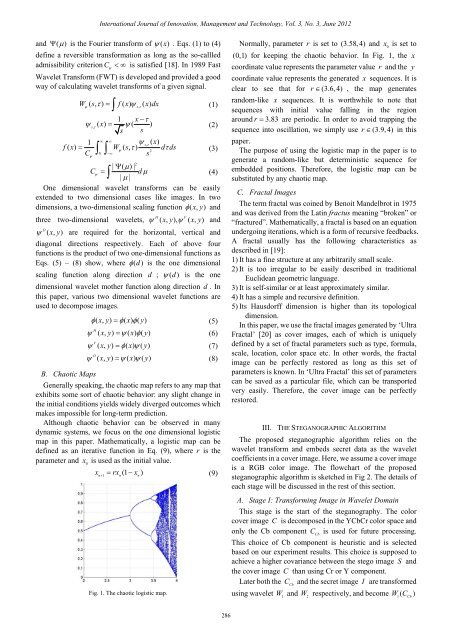
International Journal of Innovation, Management <strong>and</strong> Technology, Vol. 3, No. 3, June 2012 <strong>and</strong> Ψ ( μ) is the Fourier transform of ψ ( x) . Eqs. (1) to (4) define a reversible transformation as long as the so-callled admissibility criterion C ψ
International Journal of Innovation, Management <strong>and</strong> Technology, Vol. 3, No. 3, June 2012 <strong>and</strong> W ( I ). Here W <strong>and</strong> W are determined by the key <strong>and</strong> 2 1 2 they may or may not be necessarily the same. One benefit of this design is to achieve a larger key space. Unless the correct wavelet mother function W is used, one cannot extract the 1 exact embedded secret information from a cover image; unless the correct wavelet mother function W is used, one 2 cannot restore the secret information from extracted secret information in the spatial domain. Stage I Stage II A DV Secret <strong>Image</strong> Ι W(Ι) A DV DWT W(SCb) DH DD DH DD Logistic Map Selecting Positions Energy Equalization Embedding Data IDWT Stage III W(CCb) SCb A DV DWT DH DD IYCbCr CCb Cover <strong>Image</strong> C YCbCr CCr CY Stego <strong>Image</strong> S Fig. 2. The flowchart of the proposed steganographic scheme. B. Stage II: Secret Data Embedding This stage is the core of the steganography. It embeds the transformed secret image W 2 ( I ) in the transformed cover image W ( C ) . 1 Cb First, the initial value x <strong>and</strong> the parameter value r of the 0 logistic map in Eq. (9) are determined by the key. Based on the number of coefficients in W 2 ( I ) , the logistic map generates an equal length chaotic sequence Seq. However, this sequence Seq has to be quantized before used for extracting wavelet coefficients in W ( C ) . The number of 1 Cb quantization scales N is calculated via Eq. (10), where #(.) computes the number of elements <strong>and</strong> dt . rounds the number towards to zero. Then Seq is quantized <strong>with</strong> respect to the bin numbers of the N equal-length bins in (0,1) , namely ⎛ 1 ⎤ ⎛k−1 k ⎤ ⎛ N −1 ⎞ B = 0, , , B , , , B ,1 1 ⎜ k N N ⎥ = ⎜ = N N ⎥ ⎜ N ⎟ ⎝ ⎦ ⎝ ⎦ ⎝ ⎠ Consequently, Seq is translated to a r<strong>and</strong>om-like sequence Seq composed of only numbers from 1 to N . N However Seq is still not the sequence which can be used N to extract wavelet coefficient in W ( C ) . Seq is calculated 1 Cb N for partial sum <strong>and</strong> the Seq is obtained according to Eq. (11). c Seq is used to extract wavelet coefficients in W ( C ) . It is c 1 Cb worthwhile to note that W ( C ) is composed of four regions 1 Cb (see Fig. 2), namely approximation region A (passed by the low-pass filter along y <strong>and</strong> followed by the low-pass filter along x ), horizontal-details region DH(passed by the low-pass filter along y <strong>and</strong> followed by the high-pass filter along x ), vertical-details region VH(passed by the high-pass filter along y <strong>and</strong> followed by the low-pass filter along x ), <strong>and</strong> diagonal-details DD (passed by the high-pass filter along y <strong>and</strong> followed by the high-pass filter along x ). We keep region A but choose to substitute coefficients in DH, DV <strong>and</strong> DD by the wavelet coefficients of W ( I ) . This is the reason 2 why Eq. (10) contains a factor of 3/4. In fact, the region A can be considered as the DC component of the image C . Cb Any change in this DC component may lead to big changes in the future. However, DH, DV <strong>and</strong> DD are more or less about the edge strength of C . Fractal cover images normally have Cb a large number of edges <strong>and</strong> rely on the DC component of the image to have the fractal-like patterns. ⎢ 3 × #( C Cb ) ⎥ N = ⎢ ⎥ (10) ⎣ 4 × #( W ( I)) 2 ⎦ k Seq ( k) = ∑ Seq ( k) (11) c i= 1 N The selected coefficients in W ( C ) are uniquely determined 1 Cb by Seq <strong>and</strong> we named the set of the chosen coefficients as c P . Eq. (12) is used as the ratio of energy in set X to that in set Y , where E(.) represents the energy function. 2 EX ( ) x RXY ( , ) = 2 EY ( ) = ∑ ∑ (12) y We then compute L = R( P, W ( I)) <strong>and</strong> lift wavelet 2 coefficients correspondingly, Consequently, the lifted energy LE( W ( I )) approximately match the energy of the original 2 EP ( ). Finally, we call these modified wavelet coefficients W ( S ) . 1 Cb C. Stage III: Transforming <strong>Image</strong> Back to Spatial Domain Parallel to the Stage I, the main task of the Stage III is to inverse transform everything in the wavelet domain to the spatial domain. W ( S ) is inverse wavelet transformed to the spatial 1 Cb domain <strong>and</strong> becomes the image S Cb . The S Cb is used to replace the original Cb component C Cb for the color cover image C . Eventually, the component set { C , S , C } is converted Y Cb Cr from the YCbCr color space to the RGB color space. IV. SIMULATION RESULTS AND DISCUSSION Our computer simulation is run in the MATLAB R2009a environment under Window XP operation system <strong>with</strong> 3GB memory <strong>and</strong> Core 2 Quad 2.6GHz CPU. The key we used in the simulation has the format of { x , r, width, height, db #, db #}, where x <strong>and</strong> r are used in 0 C I 0 the logistic map for generating the embedding/ extracting positions; width <strong>and</strong> height are used to reform the rebuilt 287