Lab script - Jodrell Bank Centre for Astrophysics

University of Manchester
Department of Physics and Astronomy
3rd Year Laboratory
An introduction to radio telescopes and pulsar astronomy
http://www.jb.man.ac.uk/research/pulsar/lab
1. OUTLINE
Note that this experiment requires a reasonable aptitude for programming
in C or C++.
This experiment runs for four weeks. You will spend the Tuesday of each week carrying out experimental
and observational work at Jodrell Bank and the Thursdays on carrying out data analysis and background
reading in Manchester. The topics covered are as follows:
Week 1: An introduction to radio telescopes. You will measure the beam shape of the telescope
by performing scans across a strong radio source. Using the 42-ft telescope you will make relative flux
density measurements of some strong radio sources compared with a calibration noise source.
Weeks 2 & 3: An introduction to pulsar astronomy. You will use some existing data obtained
with the 76-m Lovell radio telescope to search for the presence of a radio pulsar and to measure its period.
To do this, you will write a programme and use simple Fourier analysis techniques. You will then use
existing data obtained with the 42-ft telescope on the ‘Crab pulsar’ to measure pulse arrival times at the
observatory over a period of a few days. These times must be corrected to the barycentre of the Solar
System to obtain the true period and its first derivative. This entails writing a second computer program
to analyse and correct the arrival time data. From the results the age and surface magnetic field of the
neutron star in the Crab Nebula can be deduced.
Week 4: Determining the ‘dispersion measure’ of a pulsar. Using the 42-ft telescope you will
measure pulse arrival times as a function of observing frequency and hence calculate the dispersion
measure. You can then determine the approximate distance to the pulsar.
It is most important that you keep a careful running record of your observational and
analytical work in your laboratory notebook. To complete the experiment properly, you
will need to tackle all the problems set out in bold font in this script.
1 Background reading
Some suggestions for background reading:
• Background information about pulsars is given in the article by Lorimer “Radio Pulsars: An Observer’s
Perspective” and a more detailed review which both can be found online 1 .
• See http://www.jb.man.ac.uk/research/pulsar/Education/
• Textbook “Handbook of Pulsar Astronomy” by Duncan Lorimer and Michael Kramer
• Textbook “Pulsar Astronomy” by Lyne & Graham-Smith
1 Radio Pulsars: An Observer’s Perspective: http://www.jb.man.ac.uk/research/pulsar/lab/lorimer99.pdf
Detailed review: http://relativity.livingreviews.org/Articles/lrr-2001-5
1

2. AN INTRODUCTION TO RADIO TELESCOPES
The primary reflecting surface of the telescope is a paraboloid of revolution which focusses the incoming
radiation onto the ‘feed’ aerial (see Fig. 1). Its action is, therefore, to turn plane waves into spherical
waves whose centre of curvature is at the primary focus. In order to maximise the efficiency of the
telescope, power reflected from near the edges of the dish must be collected by the feed. However, in
so doing unwanted power will also be picked up from the surroundings of the telescope; this is termed
‘spillover’. The response of the feed as a function of direction is therefore tailored to maximise the
ratio between the ‘gain’ of the telescope and the overall system noise temperature to which the spillover
contributes (see below).
θ
Feed
x
Figure 1: Schematic diagram of a radio telescope
2.1 The Beamshape and the Aperture Illumination
To understand the response of the telescope as a function of direction it may be easier to think about
waves being transmitted from the feed and reflected off the paraboloid and into space; the telescope’s
characteristics are identical when transmitting or receiving (the reciprocity theorem). The waves from the
feed excite changing currents in the reflecting surface and these in turn result in electromagnetic waves
being radiated in the forward direction; the overall far field pattern of the telescope (its voltage polar
diagram) is a combination of these plane waves. This is Fraunhofer diffraction. The aperture distribution
A(x) of surface currents is related to the voltage polar diagram, P(θ), by a Fourier Transform relationship.
In one dimension:
P(θ) =
∫ D/2
−D/2
A(x)e i(2πx/λ)θ dx,
where D is the diameter of the telescope, and λ is the observing wavelength (consult Hecht ‘Optics’,
Chapter 10).
An equivalent way to understand the ‘Fourier pair’ relationship between the aperture distribution and the
far field pattern is to imagine the aperture distribution being made up from a set of sinusoidal standing
waves (effectively a set of notional diffraction gratings across the aperture). By Fourier’s Theorem any
such spatial distribution can be constructed out of a weighted set of sinusoids (spatial Fourier components).
Each sinusoidal diffraction grating of spatial wavelength d gives rise to two plane waves (at ±θ
where θ = λ/d) and the integrated effect of the plane waves from all the spatial Fourier components in
the aperture produces the voltage polar diagram. Note the inverse relation between θ and d which is
characteristic of a Fourier pair – the smaller is the spatial dimension involved, the larger is the angle
over which waves are radiated. The larger is the telescope diameter, the longer are the spatial Fourier
components which can can be ‘fitted in’ to the aperture and hence the more power which is radiated at
small angles.
N.B. Since the receiving system you are using responds to the total power rather than the complex
voltage, the beam pattern you measure by scanning the telescope is called the power polar diagram of
the telescope.
2

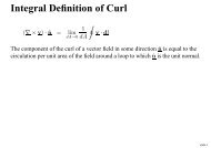
The Fourier transform of a disk, the geometrical shape of the aperture of the telescope, is called a firstorder
Bessel function and the square of this function, giving the power polar diagram, has a full-width
at half maximum of 1.02λ/D radians, where D is the diameter of the telescope and λ is the wavelength.
Scan the telescope across the strong source Cass A (see Appendix A, but ask the lab demonstrator
for some additional instructions first) and measure the width of the power polar
diagram (power polar representation of the telescope beam) between half-power points. Is
this consistent with the known diameter of the telescope? Can you explain any differences?
2.3 Calibration and Noise Temperature Measurements
Noise Temperature: Essentially all the signals we deal with in radio astronomy are pure random noise.
The parameter most often used to characterise these signals is the ‘noise temperature’ T (measured in
K) which is directly proportional to mean noise power available from a resistor at temperature T. From
the theorem of equipartition of energy there are kT/2 Joules of energy associated with each ‘degree of
freedom’ of the system, i.e. in each Hz and in each of the two polarisation states. Thus the power per
unit bandwidth is kT Watts Hz −1 and over a bandwidth B Hz the total power available is kTB Watts.
Absolute calibration measurements in radio astronomy are therefore made using ‘hot and cold loads’
which are resistors at well-defined temperatures (e.g. liquid He, liquid N and room temperature).
After amplification, the random noise signals, which have a zero mean, are turned into a more useful form
by a detector. Usually in radio astronomy we use a device (most simply based on a diode operating on the
bottom part of its characteristic curve) which responds to the square of the input voltage i.e. to the power
of the random signal integrated over an appropriate period. In a basic receiver this period could be set
by an RC ‘time constant’. Because the statistical nature of the input signal there is a random fluctuating
component in the detected signal (see Fig. 2) whose magnitude is ∝ T/ √ Bτ where τ is the time over
which the signal is averaged. (Note that this is akin to the fluctuations ∝ √ N in Poisson statistics).
Thus the accuracy of the measurement of the mean power is increased by increasing the signal bandwidth
and the averaging time.
Fluctuations, rms= Tsys
Bt
Power Output
Tsys
Time
Figure 2: The noisy signal after square-law detection
The total noise power at the output of the receiver, often called the ‘system noise temperature’ T sys , has
several contributions:
i) T source , the desired contribution coming from the radio source.
ii) T sky , the contribution from the sky around the source.
iii) T spillover , the contribution from the ground around the telescope.
iv) T rec , the noise generated in the receiver electronics.
Because we are dealing with random noise signals the powers add i.e.
T sys = T source + T sky + T spillover + T rec .
3

Figure 3: The spectrum of a sequence of pulses from a pulsar, taken from Fig. 3.3 of “Pulsar Astronomy”
by Lyne and Smith (1998).
For these observations T sys ≈ 100K, T sky ≈ 20 K and T spillover ≈ 10 K. The ‘aperture efficiency’ of the
42-ft telescope is ∼ 55% (i.e its effective collecting area is 55% of its physical area). This translates to a
sensitivity of 0.026 K Jy −1 and therefore if the source has a flux density of 100 Jy the noise contribution
corresponds to 2.6 K. Note that 1 Jy corresponds to 10 −26 W m −2 Hz −1 and that it is a measure of the
power falling on unit area per unit bandwidth.
The flux density at 610 MHz of the calibration sources of interest to your observations are: Cassiopaeia
A, 3595 Jy (epoch 1990, decreasing at 1.03 % per year) and Cygnus A, 3555 Jy. Their contributions to
T sys are therefore ≈ 93K and ≈ 92K respectively. These are the strongest sources in the sky; usually
radio astronomers observe much weaker sources whose contribution is therefore ≪ T sys .
If the signal bandwidth of your receiving system is 8 MHz, what averaging time must be
used in order to detect a 1 Jy source with a signal-to-noise ratio of 10:1?
Scan the telescope across the radio sources Cass A and Cygnus A (provided they are above
the horizon) and compare the deflection on the pen recorder (which measures the total
power from the system) with that from the ‘CAL’ signal. Establish the magnitude of CAL
in Jy. Make scans across one or both of Taurus A (the Crab Nebula) and Virgo A and use
the calibration you have just derived to establish the flux density of these sources. Quote
the errors on your answers.
3. AN INTRODUCTION TO PULSAR ASTRONOMY
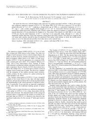
Pulsars were discovered in 1967 by Bell & Hewish at Cambridge. Within a year it was accepted that they
were rotating neutron stars. The 76-m Lovell telescope, as well as the 42-ft telescope, are more flexible
instruments for studying known pulsars and for finding new ones than the dipole array used by Bell &
Hewish. A significant part of the subsequent detective work on pulsars has therefore been carried out at
Jodrell Bank.
3.1 Detection of an unknown pulsar and measurement of its period
One of the greatest challenges in pulsar astronomy is the discovery of pulsars of unknown periodicity.
Only once the period is known can the pulsar data be “folded” to produce high signal-to-noise ratio
profiles which can be used to study the pulsar in detail. This search process is now carried out by
inspection of the power spectrum of the data which will show delta functions at the fundamental rotation
frequency of the pulsar and its harmonics, the number of harmonics being roughly equal to P/2W, where
P is pulse period and W is the pulse width (see figure 3). From the frequency of the Nth harmonic, ν N ,
4

the frequency of the fundamental and its error can be estimated as (ν N ± 0.5∆ν)/N, where ∆ν is the
frequency interval in the spectrum and equal to 1/T, where T is the total duration of the time sequence.
Thus the most accurate estimate of the frequency can be obtained from the highest clearly detectable
harmonic.
Write a computer program to perform the Fourier transform of a time sequence of samples
obtained with the 76-m Lovell radiotelescope (ask your lab demonstrator for a template for
the computer code and data). By graphical inspection of the resultant amplitude spectrum
(obtained by calculating the amplitude of each of the complex numbers in the spectrum),
estimate the frequency and width of the pulses in the time sequence.
3.2 Pulse arrival times from the Crab pulsar
Much can be inferred about the physics of neutron stars and their binary companions (if present) from
an analysis of the precise arrival times of the pulses. You will be supplied with a set of profiles obtained
with the 42-ft telescope, on the powerful pulsar in the Crab Nebula. The data were taken by folding
the data using an approximate period, on two separate days with a gap of several days between them.
Before one can use these data for physical interpretation they must be corrected for the motion of the
observatory around the Sun, i.e. the pulse train should appear to have been collected at a fixed point in
space. The most convenient point to use is the centre of mass of the Solar System, its barycentre.
Data on the position of the centre of the Earth with respect to the barycentre are given in the Astronomical
Almanac and will be provided by the lab demonstrator. However, since positions are only given once per
day, it is necessary to interpolate between the data points to be able to correct the arrival times to a
sufficient precision. The typical error in the arrival time of a pulse in the raw data is ∼ 0.2 milliseconds,
and the interpolation error must be less than this. An additional correction is required because the
observatory is not located at the centre of the Earth! It has a very simple form: r sin(ǫ)/c, where r is
the radius of the Earth, ǫ is the elevation of the source above the horizon and c is the velocity of light.
Justify the form of this correction with a simple diagram. The actual elevation of the pulsar is
given for each profile in the data set with which you are supplied.
Draw a diagram which demonstrates the principles of the barycentric correction. Write a
computer program to perform the interpolation between the barycentre positions supplied
by the lab demonstrator using one of the Lagrange multi-point formulas (see Appendix C)
after determining which one is suitable. Determine the light travel times from the Earth’s
centre to the Solar System barycentre. Make the further correction dependent on the
elevation of the pulsar.
It is straightforward to determine the raw arrival times (defined as the time the pulse arrives after the
beginning of the scan) from the data provided by the lab demonstrator. These data are the input data
to a computer program which determines an accurate period for the individual days. The philosophy
behind your program can be as follows:
By definition any two arrival times should be separated by an integer number of pulse periods. However,
if the current estimate of the pulse period is incorrect, dividing the time separation by the period will
not produce an integer. Provided the estimate is not far wrong, taking the nearest integer and dividing
the separation by this integer will yield a more accurate estimate of the pulse period. Ask the lab
demonstrator for an initial estimate for the period of the Crab pulsar. This value is accurate enough to
obtain the correct integer number of periods over a 10-min interval. Use the current period estimate to
calculate arrival times throughout the day and subtract these from the raw data. These ‘residuals’ will
systematically grow throughout the day. Plot the residuals against time and use the slope (determined
by least-squares fitting) to make a better estimate of the pulse period. By iterating around this loop it
should be possible to eliminate systematic trends in the plot of residuals and hence to arrive at the best
estimate of the period for that day.
5

Write a computer program to determine an accurate pulse period for each of the two
days; include the barycentric correction program as a subroutine. Determine the period
derivative and hence estimate the age of the pulsar and its surface magnetic field. Quote
the errors on your answers.
3.3 Measurement of pulsar dispersion measures
On its way to the Earth the pulsed radiation passes through ionised plasma in the interstellar medium
(ISM). The refractive index of plasma is a function of frequency and hence the radiation experiences a
frequency dependent delay – i.e. the ISM is dispersive. From the difference in arrival time as a function
of frequency one can calculate the ‘dispersion measure’, the integrated electron number density along the
line-of-sight to the pulsar i.e.
DM =
∫ earth
pulsar
n e · dl.
More details about the frequency dispersion in pulse arrival time are given in Appendix D. The dispersive
effect of the ISM causes initially sharp pulses to become smeared in addition to suffering an overall delay,
when observed with a receiver with a finite bandwidth. This pulse-smearing effect must be removed by
special-purpose electronics (‘de-dispersers’) in order to restore the original signal-to-noise ratio.
610 MHz
Feed
Amplifier
~
290 MHz 580 MHz
X2
X
Mixer
Synthesiser
Multiplier
30 MHz
Amplifier
Detector
Output
Figure 4: Schematic diagram of the heterodyne receiver
The receiver on the 42-ft telescope is a heterodyne one. The noise signals collected by the telescope are
‘mixed’ with a pure sinusoidal local oscillator (LO) signal. The difference signals are lower frequencies
which are more convenient for filtering and amplification and passing along long lengths of cable from
the focus box to the observing room. A simplified diagram of your receiver is shown in Fig. 4. The LO
signal is generated in a frequency synthesiser whose output frequency can be changed at will. Note that
the synthesiser signal for the first LO is doubled in a non-linear ‘multiplier’.
Measure the change in arrival time of pulses as a function of frequency from observations
at ≥ 3 frequencies (ask the lab demonstrator for instructions). Use the relevant equation
in Appendix D to determine the dispersion measure of the pulsar. Assuming a value of
the mean electron density in the ISM of 0.03 cm −3 calculate the distance of the pulsar.
Compare your value with the published value.
6

Appendix A: Making scans with the 42-ft telescope
The 42-ft telescope is controlled with a computer called arthur. After consulting the lab demonstrator,
the following procedure should be followed to make a scan:
1. The 42-ft telescope is used most of the time for scientific pulsar observations, so it is important to
stop those observations first before you start. This is done in the program called menu2 (NEVER
RUN menu INSTEAD OF menu2!). Commands are entered by pressing the “DO” key, which you
can find on the keyboard. Enter the commands “abort” and “close”. Use the ’-’ key on the numeric
keypad to go back in a menu.
2. The telescope is controlled via the program “telc”, which will ask which telescope you want to
opperate. Type “42ft” and you see the time (UT and ST), the pointing position (actual and
demanded), the requested coordinates, source offset and offset rates. To move to for instance CAS
A press the DO key and type its coordinates: “2000 23:23:26.4 58:49:34.0”, where the 2000 means
you entered the coordinates with respect to epoch 2000. To scan over the source you can press the
DO-key and type “offset 5 0” to start with an azimuth offset of 5 ◦ (and an elevation offset of 0 ◦ ).
Then enter the command “offrate -2.5 0” to scan back in azimuth with 2.5 deg/min. When the
scan is completed you can stop scanning by entering the commande “offrate 0 0”.
3. You will record the signal using a chart recorder. A speed of 30mm/min should give a good plot.
DO NOT WASTE PAPER, so stop the recorder if you are not recording useful data and do not use
excessive speeds. MAKE NOTES IN YOUR LABSCRIPT OR ON THE CHART WHAT SPEED
SETTING WAS USED FOR WHICH CHART! Most likely you should adjust the offset and scale
settings on the chart recorder to get a good plot.
7

Andrew Lyne and Peter Wilkinson, with modifications from Dunc Lorimer, Patrick Weltevrede, Ben
Stappers & Chris Jordan.
Last modified: September 2013
11