Lab I: Heat diffusion
Lab I: Heat diffusion
Lab I: Heat diffusion

You also want an ePaper? Increase the reach of your titles
YUMPU automatically turns print PDFs into web optimized ePapers that Google loves.
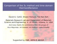
<strong>Heat</strong> <strong>diffusion</strong><br />
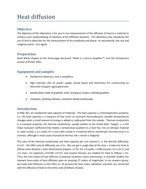
Objective<br />
The objective of this laboratory is for you to use measurements of the <strong>diffusion</strong> of heat in a material to<br />
enhance your understanding of solutions of the <strong>diffusion</strong> equation. This laboratory also introduces the<br />
use of lock‐in detection for the measurement of the amplitude and phase—or equivalently, the real and<br />
imaginary parts—of a signal.<br />
Preparation<br />
Read White Chapter 8; the three‐page document “What is a lock‐in amplifier?”; and the introductory<br />
section of Parker 1961.<br />
Equipment and samples<br />
• Pyroelectric detectors, lock‐in amplifiers.<br />
• High intensity LED; dc power supply; bread board and electronics for constructing an<br />
electronic chopper; signal generator.<br />
• Sample disks made of graphite, steel, and glassy carbon; colloidal graphite.<br />
• Computer, plotting software, computer‐based oscilloscope.<br />
Introduction<br />
In MSE 307, we studied the heat capacity of materials. The heat capacity is a thermodynamic property;<br />
i.e., the heat capacity is a measure of how much an intensive thermodynamic variable (temperature)<br />
changes when a small amount of energy is added or subtracted from the sample. Thermal conductivity<br />
is a transport property; the thermal conductivity, usually written as the Greek letter “kappa” κ, is the<br />
linear transport coefficient that relates a temperature gradient to a heat flux. For an isotropic material<br />
or cubic crystal, κ is a scalar; for a non‐cubic crystal or a material with an anisotropic microstructure κ is<br />
a tensor, although in most cases of practical interest, the κ tensor is diagonal.<br />
The ratio of the thermal conductivity and heat capacity per unit volume C, is the thermal diffusivity,<br />
D=κ/C. The MKS units of diffusivity are m 2 /s. We can get a rough idea of the time τ it takes for heat to<br />
diffuse some distance L from dimensional analysis τ=L 2 /D. For a Si wafer, L=500 microns, D=1 cm 2 /s, and<br />
τ=2 msec. For polymers, D=0.001 cm^2/s and several minutes are needed for heat to diffuse 1 cm.<br />
Thus, the time‐scales of heat <strong>diffusion</strong> in practical situations varies enormously. In scientific studies, the<br />
relevant time‐scales of heat <strong>diffusion</strong> span an amazing 27 orders of magnitude: in my research group,<br />
we study heat <strong>diffusion</strong> in thin films on 10 picosecond time scales; planetary scientists are concerned<br />
with the <strong>diffusion</strong> of heat on the time‐scale of billions of years.
Thermal conductivity can be measured directly but the most widely used experimental method for<br />
determination of thermal conductivity, flash diffusivity, actually measures thermal diffusivity. Thermal<br />
conductivity is then derived from diffusivity using κ=DC.<br />
Session 1: Measure the frequency response of the pyroelectric detector<br />
using a chopped LED light source<br />
• Build an “electronic chopper” from a dc power supply, signal source and a transistor. A<br />
circuit diagram is shown below.<br />
• Allow a small amount of the light from the modulated light‐emitting diode (LED) to fall on<br />
the pyroelectric detector. As you did for the pyrometry lab in MSE 307, observe the<br />
amplitude and shape of the signal but now go a step further and measure the signals using a<br />
lock‐in amplifier and determine the amplitude and the phase of the frequency response of<br />
the detector. (The range of frequencies should be 1 to 100 Hz; your plots should use a log<br />
scale for the frequency so when you collect the data think about spacing the data points by<br />
a constant factor rather than a constant interval.) In the high frequency limit, the amplitude<br />
should decrease as 1/f and the phase should be –π/2 radians.<br />
Session 2: Measure the thermal diffusivity of a material using heating by<br />
a chopped LED and a pyroelectric detector<br />
• Measure the thermal diffusivity of a sample (currently 0.8 mm thick carbon‐coated steel) by<br />
illuminating one side of the sample with the modulated LED heat source and measuring the<br />
amplitude and phase of the temperature response on the other side of the sample using the<br />
pyroelectric detector. The sample is installed in place of the window on the pyroelectric<br />
detector. Place the LED a few mm away from the sample.<br />
• To do this, you will need to measure the amplitude and phase of the signal generated by the<br />
pyroelectric detector with the lock‐in amplifier. The amplitude and phase of the<br />
temperature of the back‐side of the sample is given by this response function measured<br />
with the sample installed divided by the response function of the detector measured in the<br />
1<br />
first session. Compare your results to the functional form given in lecture ( qd sinh( qd))<br />
−<br />
where qd=iωd 2 /D, d is the sample thickness, and ω is the angular frequency.<br />
• Repeat using a different thickness of sample and determine the thermal diffusivity of the<br />
samples using the condition qd=2.2 when the real and imaginary parts of the temperature<br />
response are equal.<br />
January 25, 2009
Instrument procedures<br />
Detector and oscilloscope<br />
We use the SPH‐CM‐Test pyroelectric detector to measure the power of radiation emitted. The heart of<br />
the detector test box is a 5 mm diameter LiTaO 3 detector. The detector generates a voltage signal by<br />
detecting a temperature change due to incoming radiation with linear response up to 40,000 V/W. The<br />
detector test box has a BaF 2 window that is transparent to visible and IR radiation (up to 17.5 μm) to<br />
block air flow.<br />
To collect the data, we use a DS1M12 oscilloscope. Turn on the detector and start the EasyScope II<br />
program. You want to trigger ChB with the sync output of the chopper. Adjust the T/Div and V/Div<br />
knobs to see a clear image of the signal. Adjust Gnd level if necessary. Pressing Meter A button will<br />
display useful readings, which you can customize by pressing configure.<br />
Circuit diagram for electronic chopper<br />
Square Wave<br />
Generator<br />
LED<br />
NPN BJT<br />
100 ohm<br />
DC Power<br />
Supply<br />
January 25, 2009