Imaging electron motion with attosecond time resolution

Imaging electron motion
with attosecond time resolution
Peter Abbamonte, UIUC
Collaborators:
Tim Graber, Advanced Photon Source
Wei Ku, Brookhaven National Laboratory
James Reed, UIUC
Serban Smadici, UIUC
Young Il Joe, UIUC
Gerard Wong, UIUC
Robert Coridian, UIUC
Ken Finkelstein, Cornell University
Sol Gruner, Cornell University
Abhay Shukla, Université Pierre et Marie Curie
Jean-Pascale Rueff, Synchrotron SOLIEL
Funding: Office of Basic Energy Sciences, U.S.
Department of Energy #s DE-FG02-06ER46285 &
DE-AC02-98-CH10886

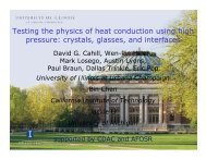
Femtochemistry
1
*
2
2
NaI( Σ0)
→ [Na ⋅⋅⋅ I] → Na( S
1/2)
+ I( P3/
2)
P. Cong, et. al., J. Phys. Chem., 100, 7832 (1996)
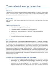
“Is there another domain in which the race against time can continue to be pushed Subfemtosecond
or attosecond (10 -18 s) resolution may one day allow for the direct observation
of the electron’s motion. … In the coming decades we may view electron rearrangement,
say, in the benzene molecule, in real time.” – Ahmed Zewail, 2000 Nobel Address

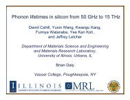
Attoscience
Reproduced from Drescher, et. al., Science, 291 1923 (2001)
• Events preceding photofragmentation
• Quasiparticle “birth” in semiconductors
• Inner shell processes (shape resonances)
• Electron transfer chemistry

Press

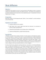
Why not energy domain - photoabsorption
∆t = 100 attosecond, ∆E·∆t = ħ /2 ⇒
∆E = 6.58 eV
grating
slit
counter
lamp
specimen
I( ω)
= exp[ −µ ( ω)
L]
µ ( ω)
⇒ ε(
ω)
ε(
ω)
−1
χ
e(
ω)
=
4π
P( ω)
= χ ( ω)
E(
ω)
e
P(t)
E(t)
∫ ∞ −∞
P( t)
= dt′
χ ( t − t′
) ( t′
e
E )
t 0
time (as!)
“…energy-domain measurements on their own are – in general – unable to provide detailed insight
into the evolution of multi-electron dynamics.” – M. Drescher, et. al., Nature (2002)

Inelastic x-ray (or n + or e – ) scattering
(k 2 ,ω 2 )
(k 1 ,ω 1 )
Fluctuation-Dissipation theorem:
Bell Jar
I(k,ω) ~ – Im[χ(k,ω)]
k = k 1 – k 2
Pendulum
ω = ω 1 – ω 2

Inelastic x-ray (or n + or e – ) scattering
Couple light to electrons
(Lorentz force law)
Be sure to second-quantize to get photons
Multiply out to get interactions
Do perturbation theory (1st Born approximation)
Turns out to be a Green’s function

What is χ(k,ω)
χ(k,ω) :
• density-density Green’s function
• density propagator
• susceptibility
Describes how disturbances in electron density travel about the medium.
(x,t)
Causality
Same as a pump-probe experiment.
Dynamics is dynamics
(0,0)

“Phase problem” and the arrow of time
Cannot invert with only Im[χ(k,ω)]
Im[ω]
× × × × × × × × × Re[ω]
× × × × × × × × ×
• χ(x,t) = 0 for t < 0
• Raw spectra do not really describe dynamics – no causal information
• Must assign an arrow of time to the problem. Permits retrieval of χ(x,t) –
view dynamics explicitly.

IXS - practical
Backscattering
analyzer
Monochromatic
beam
White beam from APS undulator
scattering
angle
Specimen (H 2
O)
K. D. Finkelstein, P. Abbamonte, V. O. Kostroun, Proc. SPIE Int. Soc. Opt. Eng. 4783, 139 (2002)

Plasma oscillations in water
– Im[χ(k,ω)] (as/Å 3 )
• 8 valence electrons / molecule
• ρ = 1 g/cm 3 ⇒ n = 0.20 e/Å 3
• ω p
= √(4πne 2 /m) = 16.6 eV
• k max
= 4.95 Å -1 ⇒ dx = 0.635 Å
• ω max
= 100 eV ⇒ dt = 20.7 as

Problems
Problem #1:
Im[χ(k,ω)] must be defined on infinite ω interval for continuous time interval
Solution:
Extrapolate.
Side effects:
• χ(x,t) defined on continuous (infinitely narrow) time intervals.
• Time “resolution” ∆t N = π/Ω max
• Ω max plays role of pulse width.

Problems
Problem #2:
Discrete points violate causality
Im[χ(k,ω)] must be defined on continuous ω interval. Periodicity incompatible with
causality.
Solution:
Analytic continuation (interpolate)
Side effects:
• χ(x,t) defined forever. Vanishes for t < 0.
• Repeats with period T = 2π/∆ω = 13.8 femtoseconds
• ∆ω plays role of rep rate

Nyquist’s (critical sampling) theorem
f(t)
|f(ω)| 2
t
− ω max
ω max
ω
ω N = 2 ω max
Nyquist frequency
ω too small
⇒ aliasing
∆t N
= 20.7 as
∆x N
= 0.635 Å

Disturbance from a point perturbation.

Disturbance from a point perturbation – frame-by-frame
0.1 Å -6
Units Å -6
clipped at 1 Å -6
0.005 Å -6
∆t N
= 20.7 as
∆x N
= 0.635 Å
• Events transpire in 350 as – light travels 100 nm in vacuum
• Causality Analytic properties Rise of entropy Arrow of time

Compound sources
(x,t)
(x 0 ,0)
(x 1 ,0)

Compound sources – oscillating dipole

Compound sources – wake from 9 MeV Au ion
• Phys. Rev. Focus, 14 June 2004
• Chemical & Engineering News, 82, 5 (2004)

Excitons: Frenkel vs. Wannier
conduction band
valence band
Frenkel (Xe, Organics, …)
Wannier (Si, Ge, Cu 2
O, …)
J. Frenkel, Phys. Rev., 37, 17 (1931) G. H. Wannier, Phys. Rev., 52 191 (1937)

Alkali halides – an intermediate case
“Excitation” model
Dexter, D. L., Exciton models in alkali halides, Phys. Rev. 108,
707-712 (1957)
It’s all just Wannier
Hopfield, J. J., & Worlock, J. M., Two-quantum absorption
spectrum in KI and CsI, Phys. Rev. 137, A1455-A1464 (1965)
GW correction / Solve Bethe-Saltpeter eqn.
Rohlfing, M., & Louie, S. G., Electron-hole excitations in
semiconductors and insulators, Phys. Rev. Lett. 81, 2312-2315
(1998)
Discovery of excitons in alkali halides
Hilsch, R., & Pohl, R. W., Über die ersten ultravioletten
Eigenfrequenzen einiger einfacher kristalle, Z. Physik 48, 384-396
(1928)
Marginal case btwn. Frenkel and Wannier
Mott, N. F., Conduction in polar crystals. II. The conduction band and
ultra-violet absorption of alkali halide crystals, Trans. Faraday Soc.
34, 500-506 (1938)
Electron transfer model
Overhauser, A. W., Multiplet structure of excitons in ionic crystals,
Phys. Rev. 101, 1702-1712 (1956)

Frenkel vs. Wannier in time-domain IXS
Wannier’s Excitonic Basis:
| R, R + β >
Excitons come from diagonalizing
∑
K
ββ ′
′
R
−i
⋅R
H ( K) = e < R, R + β | H | 0, β >
For Frenkel exciton, dominated by one term:
∑
K
R
( ) −i
⋅R
H , | | 0,0
00
K = e < R R H >
Conclusion: Frenkel exciton keeps its size / shape through its life. Wannier
changes. Inverted IXS directly sensitive to Wannier vs. Frenkel vs.
intermediate descriptions.

Result

Time response
All processes:
• Exciton
• Interband
• Plasmon
• Core levels
• Compton
scattering

Isolating the exciton
g
gap
B
( ω)
= 1 + e
k
k
g
−W
( ω−ω
)
Im[ χ ] = Im[ χ ] −g
( ω )
e,
n n gap n
⎧
Im[ χne,
n]
= ⎨
⎩
g ( ω ) ω < ω
gap n n c
Im[ χ ] ω ≥ ω
n n c
Truncated at 16.5 eV

Exciton dynamics
Frenkel limit.

Wannier functions (Ku, et. al.)

Lessons
•Exciton in LiF is Frenkel, despite the old controversy.
•No contradiction between CT and Frenkel. Lattice geometry not a
constraint.
•Causality allows solution to “phase problem” for IXS ⇒ zeptoseconds!
•Is there information in this which cannot be read off the raw spectra!
1. Extrapolation 2. Causality
• χ(x,t) useful for analyzing extended sources

Homogeneous vs. homogeneous broadening

Graphite
Wallace, Phys Rev. 71, 622 (1947)
σ,π plasmon
Compton
scattering
π plasmon