Processing Magnetometer Data in the SINGLE BEAM ... - Hypack
Processing Magnetometer Data in the SINGLE BEAM ... - Hypack
Processing Magnetometer Data in the SINGLE BEAM ... - Hypack

You also want an ePaper? Increase the reach of your titles
YUMPU automatically turns print PDFs into web optimized ePapers that Google loves.
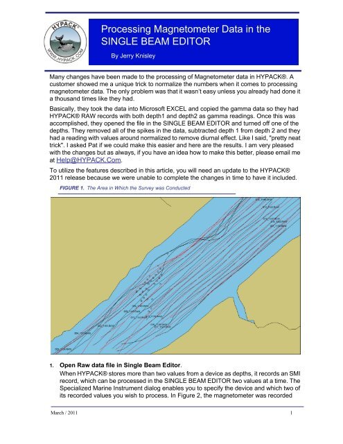
<strong>Process<strong>in</strong>g</strong> <strong>Magnetometer</strong> <strong>Data</strong> <strong>in</strong> <strong>the</strong><br />
<strong>SINGLE</strong> <strong>BEAM</strong> EDITOR<br />
By Jerry Knisley<br />
Many changes have been made to <strong>the</strong> process<strong>in</strong>g of <strong>Magnetometer</strong> data <strong>in</strong> HYPACK®. A<br />
customer showed me a unique trick to normalize <strong>the</strong> numbers when it comes to process<strong>in</strong>g<br />
magnetometer data. The only problem was that it wasn’t easy unless you already had done it<br />
a thousand times like <strong>the</strong>y had.<br />
Basically, <strong>the</strong>y took <strong>the</strong> data <strong>in</strong>to Microsoft EXCEL and copied <strong>the</strong> gamma data so <strong>the</strong>y had<br />
HYPACK® RAW records with both depth1 and depth2 as gamma read<strong>in</strong>gs. Once this was<br />
accomplished, <strong>the</strong>y opened <strong>the</strong> file <strong>in</strong> <strong>the</strong> <strong>SINGLE</strong> <strong>BEAM</strong> EDITOR and turned off one of <strong>the</strong><br />
depths. They removed all of <strong>the</strong> spikes <strong>in</strong> <strong>the</strong> data, subtracted depth 1 from depth 2 and <strong>the</strong>y<br />
had a read<strong>in</strong>g with values around normalized to remove diurnal effect. Like I said, "pretty neat<br />
trick". I asked Pat if we could make this easier and here are <strong>the</strong> results. I am very pleased<br />
with <strong>the</strong> changes but as always, if you have an idea how to make this better, please email me<br />
at Help@HYPACK.Com.<br />
To utilize <strong>the</strong> features described <strong>in</strong> this article, you will need an update to <strong>the</strong> HYPACK®<br />
2011 release because we were unable to complete <strong>the</strong> changes <strong>in</strong> time to have it <strong>in</strong>cluded.<br />
FIGURE 1. The Area <strong>in</strong> Which <strong>the</strong> Survey was Conducted<br />
1. Open Raw data file <strong>in</strong> S<strong>in</strong>gle Beam Editor.<br />
When HYPACK® stores more than two values from a device as depths, it records an SMI<br />
record, which can be processed <strong>in</strong> <strong>the</strong> <strong>SINGLE</strong> <strong>BEAM</strong> EDITOR two values at a time. The<br />
Specialized Mar<strong>in</strong>e Instrument dialog enables you to specify <strong>the</strong> device and which two of<br />
its recorded values you wish to process. In Figure 2, <strong>the</strong> magnetometer was recorded<br />
March / 2011 1
us<strong>in</strong>g <strong>the</strong> MAGNET.DLL with Gamma and Gratio recorded. (The Gratio value is <strong>the</strong><br />
current gamma read<strong>in</strong>g subtracted from <strong>the</strong> previous gamma read<strong>in</strong>g.) If <strong>the</strong>re were more<br />
values recorded <strong>the</strong>re would be more check boxes and <strong>the</strong> editor will load only <strong>the</strong> first<br />
two chosen <strong>in</strong> <strong>the</strong> list order.<br />
FIGURE 2. Specialized Mar<strong>in</strong>e<br />
Instrument Dialog<br />
In <strong>the</strong> previous version of <strong>the</strong><br />
<strong>SINGLE</strong> <strong>BEAM</strong> EDITOR, <strong>the</strong><br />
Specialized Mar<strong>in</strong>e Instrument<br />
dialog appears first. This is<br />
changed <strong>in</strong> <strong>the</strong> required,<br />
updated version so that <strong>the</strong><br />
READ PARAMETERS dialog<br />
appears before <strong>the</strong> SMI dialog.<br />
Note: If <strong>the</strong> survey was conducted with an echosounder and you want to process its data,<br />
you can advance to <strong>the</strong> normal READ PARAMETERS and select <strong>the</strong> depth device<br />
by cancell<strong>in</strong>g <strong>the</strong> SMI dialog.<br />
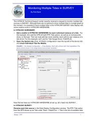
Once <strong>the</strong> data is loaded <strong>in</strong> <strong>the</strong> <strong>SINGLE</strong> <strong>BEAM</strong> EDITOR <strong>the</strong> profile will appear as it does <strong>in</strong><br />
Figure 3. Notice that <strong>the</strong> gamma read<strong>in</strong>gs are <strong>in</strong> <strong>the</strong> range of 52,000. The dipolar target<br />
between events 1290 and 1291 has a m<strong>in</strong>imum read<strong>in</strong>g of 52080.82 and a maximum<br />
read<strong>in</strong>g of 52228.23. The size of that target is not very <strong>in</strong>tuitive, but we will soon get to<br />
that po<strong>in</strong>t.<br />
2
FIGURE 3. Profile of <strong>Data</strong> <strong>in</strong> <strong>the</strong> <strong>SINGLE</strong> <strong>BEAM</strong> EDITOR<br />
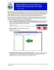
2. Mirror <strong>the</strong> data <strong>in</strong> <strong>the</strong> file.<br />
a. Access <strong>the</strong> Fill Survey dialog by select<strong>in</strong>g EDIT-FILL SURVEY.<br />
FIGURE 4. Fill Survey Dialog<br />
This is typically used to fix corrections<br />
like <strong>the</strong> draft and tide. Then Dave<br />
Maddock added <strong>the</strong> ‘Copy Depth 1 to<br />
Depth 2’ and <strong>the</strong> ‘Copy Depth2 to<br />
Depth1’ options. In most cases you<br />
will want to copy depth 1 to depth 2 so<br />
that both values are <strong>the</strong> Gamma<br />
read<strong>in</strong>gs.<br />
b. Check <strong>the</strong> ‘Copy Depth1 to Depth2’<br />
box and click [OK].<br />
March / 2011 3
3. Check to be sure that <strong>the</strong> changes were made.<br />
FIGURE 5. Enabl<strong>in</strong>g Only Depth2<br />
a. Right-click on <strong>the</strong> Profile<br />
w<strong>in</strong>dow and choose<br />
‘Display Options’.<br />
b. Disable <strong>the</strong> Depth 1.<br />
c. Enable Depth 2.<br />
d. Click [OK].<br />
The profile should now be<br />
show<strong>in</strong>g <strong>the</strong> same profile<br />
but it is blue, and actually it<br />
is Depth 2 data (Figure 6)<br />
4. Make sure that <strong>the</strong> delete operation <strong>in</strong>terpolates <strong>the</strong> sound<strong>in</strong>gs. If <strong>the</strong> DELETE<br />
REMOVES SOUNDINGS is visible <strong>in</strong> <strong>the</strong> profile w<strong>in</strong>dow, click on that phrase to change<br />
modes to ‘Delete Interpolates Sound<strong>in</strong>gs’. (If you fail to do this, you will have to redo this<br />
entire procedure.)<br />
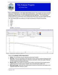
5. Highlight and delete <strong>the</strong> targets. (Figure 6) This is only go<strong>in</strong>g to delete <strong>the</strong>m from Depth<br />
2. It will actually generate a flat l<strong>in</strong>e <strong>in</strong> <strong>the</strong> editor.<br />
After dragg<strong>in</strong>g a box around <strong>the</strong> data, CTRL-I removes <strong>the</strong> data and creates a flat l<strong>in</strong>e of<br />
data but with<strong>in</strong> <strong>the</strong> average of <strong>the</strong> read<strong>in</strong>gs. This is <strong>the</strong> diurnal part of <strong>the</strong> data. You may<br />
have to do this on small sections based upon <strong>the</strong> <strong>in</strong>terference dur<strong>in</strong>g <strong>the</strong> survey l<strong>in</strong>e.<br />
I chose an easy one for this example. I dragged a box around all of <strong>the</strong> data leav<strong>in</strong>g a little<br />
outside on both ends. I could not go all <strong>the</strong> way to <strong>the</strong> end due to a change <strong>in</strong> gamma. I’ll<br />
have to edit that manually later.<br />
4
FIGURE 6. Dragg<strong>in</strong>g a Box Around <strong>Data</strong> to be Deleted .<br />
FIGURE 7. Gamma Read<strong>in</strong>gs After Spikes are Removed<br />
At first, I thought <strong>the</strong> same could be accomplished us<strong>in</strong>g -52140 as a tide value.<br />
Unfortunately, that only removes an average gamma that does not <strong>in</strong>clude an<br />
<strong>in</strong>terference <strong>in</strong> <strong>the</strong> background.<br />
You may f<strong>in</strong>d that a straight subtraction of an average Gamma read<strong>in</strong>g as tide works with<br />
your data, but I have found us<strong>in</strong>g this o<strong>the</strong>r method does a much better job of remov<strong>in</strong>g<br />
<strong>in</strong>terference and highlight<strong>in</strong>g targets.<br />
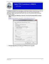
6. Return to <strong>the</strong> View Options and re-enable <strong>the</strong> Depth 1 data. Once <strong>the</strong> spikes have<br />
been removed we want to see <strong>the</strong> DEPTH 1 data as well as <strong>the</strong> DEPTH 2 data. In this<br />
screen shot I am show<strong>in</strong>g <strong>the</strong> sett<strong>in</strong>gs to show both sets of gamma read<strong>in</strong>gs, <strong>the</strong> one with<br />
spikes and our second set without <strong>the</strong>m. The screen should look similar to Figure 8. The<br />
difference between <strong>the</strong> red and blue l<strong>in</strong>es is <strong>the</strong> values that we are look<strong>in</strong>g for.<br />
March / 2011 5
6<br />
FIGURE 8. Enabl<strong>in</strong>g Both Depths 1 and 2
Whole Magnetic Analysis Tool:<br />
There is one last trick. The Profile w<strong>in</strong>dow has a new tool that is useful at this po<strong>in</strong>t. The<br />
[?] on <strong>the</strong> icon bar is a new tool to determ<strong>in</strong>e <strong>the</strong> Whole Magnetic Analysis (WMA). The<br />
idea beh<strong>in</strong>d this tool was given to me years ago <strong>in</strong> Mamma Brown’s Restaurant by Ralph<br />
Wilbanks. If you truly understand magnetometer targets, this is a tool you will use often.<br />
FIGURE 1. Whole Magnetic Analysis<br />
When you choose <strong>the</strong> tool, it changes <strong>the</strong> cursor. Place<br />
<strong>the</strong> cursor at <strong>the</strong> beg<strong>in</strong>n<strong>in</strong>g of <strong>the</strong> target you wish to<br />
measure. Click and drag <strong>the</strong> mouse to <strong>the</strong> end po<strong>in</strong>t for<br />
<strong>the</strong> target. A new dialog appears with specific<br />
<strong>in</strong>formation about that target.<br />
This tool can be used on straight gamma data without<br />
process<strong>in</strong>g it <strong>in</strong> <strong>the</strong> manner I have described here. The values will be much larger but <strong>the</strong><br />
Peak-to-Peak, Distance and time will all be <strong>the</strong> same.<br />
On <strong>the</strong> WMA dialog <strong>the</strong>re is a button to mark a target. This target is placed <strong>in</strong> a new target<br />
file, you can name <strong>the</strong> first time a target is created <strong>in</strong> <strong>SINGLE</strong> <strong>BEAM</strong> EDITOR for this<br />
session. The targets placed <strong>in</strong> <strong>the</strong> file us<strong>in</strong>g <strong>the</strong> WMA Mark Target button have a name of<br />
MAGTGT (XXX.XX). The XXX.XX will be <strong>the</strong> Peak-to-Peak value for that target.<br />
FIGURE 2. Targets Marked <strong>in</strong> <strong>the</strong> WMA Dialog<br />
In Figure 1, <strong>the</strong> targets that we recorded <strong>in</strong> <strong>the</strong> <strong>SINGLE</strong> <strong>BEAM</strong> EDITOR are easily<br />
identifiable as suitable for fur<strong>the</strong>r <strong>in</strong>vestigation or not. Also clusters of targets from<br />
separate passes with <strong>the</strong> magnetometer become readily available.<br />
7. Select EDIT -> DEP1-DEP2. This subtracts <strong>the</strong> two values and replaces depth 1 with <strong>the</strong><br />
difference. The DEPTH2 values will all be set to 0.<br />
March / 2011 7
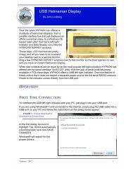
FIGURE 9. Gamma (red), Averaged <strong>Data</strong> (blue)<br />
That same dipolar target that was a m<strong>in</strong>imum of 52080.82 and a maximum read<strong>in</strong>g of<br />
52228.23 now has a m<strong>in</strong>imum of -62.04 and a maximum of 85.34. It is a lot easier to see<br />
how big that target is--147 gammas peak to peak.<br />
At this po<strong>in</strong>t, I usually go <strong>in</strong> and disable depth 2 so that I am only look<strong>in</strong>g at <strong>the</strong> data for<br />
<strong>the</strong> gamma read<strong>in</strong>gs.<br />
8. Save <strong>the</strong> edited <strong>Magnetometer</strong> data.<br />
Ano<strong>the</strong>r feature that I like to<br />
use <strong>in</strong> <strong>the</strong> <strong>SINGLE</strong> <strong>BEAM</strong><br />
EDITOR when work<strong>in</strong>g with<br />
magnetometer data is <strong>the</strong><br />
SAVE OPTIONS. This allows<br />
you to specify <strong>the</strong> extension of<br />
<strong>the</strong> data you are sav<strong>in</strong>g.<br />
Instead of <strong>the</strong> default ‘.EDT’<br />
extension I like to make it<br />
‘.GAMMA’ so I can dist<strong>in</strong>guish<br />
magnetometer data from<br />
sound<strong>in</strong>g data. To access this<br />
option, select FILE->SAVE<br />
OPTIONS. Then just save <strong>the</strong><br />
data as normal.<br />
9. Use TIN MODEL to create a 2D contour for plott<strong>in</strong>g. The f<strong>in</strong>al steps to process<strong>in</strong>g <strong>the</strong><br />
data are to TIN <strong>the</strong> data and create contours. This is ano<strong>the</strong>r area that is enhanced when<br />
process<strong>in</strong>g <strong>the</strong> magnetometer data <strong>in</strong> <strong>the</strong> manner described above. (I am not go<strong>in</strong>g to go<br />
through all of <strong>the</strong> steps to model <strong>the</strong> data us<strong>in</strong>g <strong>the</strong> TIN MODEL program. If you have<br />
questions send an email to Help@HYPACK.com and we will po<strong>in</strong>t you <strong>in</strong> <strong>the</strong> correct<br />
direction. )<br />
8
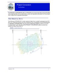
FIGURE 10. Sett<strong>in</strong>g Colors for Mag <strong>Data</strong><br />
I change <strong>the</strong> color sett<strong>in</strong>gs when I do<br />
a TIN model of <strong>the</strong> data produced with<br />
<strong>the</strong>se steps. The data is both negative<br />
and positive accord<strong>in</strong>g to whe<strong>the</strong>r <strong>the</strong><br />
gammas were above or below <strong>the</strong><br />
background data. S<strong>in</strong>ce we know if<br />
<strong>the</strong> data is negative or positive, I set<br />
all of <strong>the</strong> colors for negative values to<br />
red and all colors for <strong>the</strong> positive<br />
values to blue.<br />
This creates a nice contrast when <strong>the</strong><br />
data is output to a contour DXF file.<br />
White is <strong>the</strong> color of zero so that, <strong>in</strong><br />
Figure 11, you can easily see dipolar<br />
targets.<br />
FIGURE 11. Diurnal targets <strong>in</strong> data of an early 19th century ship wreck<br />
March / 2011 9
FIGURE 12. TIN MODEL of different gamma data (25 square miles) <strong>in</strong> 3D<br />
FIGURE 13. Contours of <strong>the</strong> <strong>Data</strong> <strong>in</strong> Figure 12<br />
10