Moisture Flux Convergence - Storm Prediction Center - NOAA

More documents

Recommendations

Info

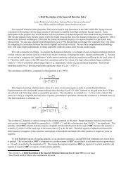
component in the Kuo convective parameterization scheme developed in the 1960s, and, (3) severe local storm prediction beginning in 1970 as a direct result of (2). A more detailed treatment of the history of each of these areas is included in the following subsections. 3.1 Calculations of precipitation in midlatitude cyclones Equation (3) can be solved for P–E, divided by the acceleration due to gravity g, and vertically integrated over the depth of the atmosphere from the surface p=p s to p=0 (Väisänen 1961; Palmén and Holopainen 1962), yielding 1 ps ∂q 1 ps 1 ps P − E = – ∫ dp – ∫ Vh ⋅∇qdp – ∫ q∇ ⋅ V dp , (6) h g 0 ∂t g 0 g 0 where the overbar represents a vertical integrated quantity. If one assumes that evaporation E is small in areas of intense precipitation and saturation, and that local changes in water vapor content are primarily those owing to advection in synoptic-scale systems (such that the first two terms on the right-hand side are in balance, see references above), then 1 p s P ≈ – ∫ q ∇ ⋅ V h dp . (7) g 0 Thus, the precipitation amount is proportional to the vertically integrated product of specific humidity and mass convergence through the depth of the atmosphere. The earliest synoptic application of (7) was from moisture budgets to estimate the large-scale precipitation in mid latitude cyclones using rawinsonde observations (Spar 1953; Bradbury 1957; Väisänen 1961; Palmén and Holopainen 1962; Fankhauser 1965). However, advances in numerical weather prediction almost certainly resulted in the phasing out of these attempts beginning in the 1960s, although the concept was theoretically sound (but also quite laborious). The case studies referenced above over the United States and the United Kingdom showed that precipitation calculated from (7) reproduced well the observed spatial pattern of precipitation and the maximum precipitation amount associated with mid latitude cyclones. 3.2 The Kuo Convective Parameterization Scheme Kuo (1965, 1974) wished to quantify the latent heat release during condensation in tropical cumulonimbus, the main source of energy in tropical cyclones. He surmised that quantification of the water vapor budget might reveal the magnitude of the vertical motion and latent heat release indirectly. He derived the vertically integrated condensation minus evaporation C – E as C − E = ( 1 − b ) gM t , (8) where b represents the storage of moisture and M t is termed the moisture accession: M t 1 ⎤ ⎢⎣ ⎡ p s = – ∫ ∇ ⋅ ( q V + h ) dp F qs . (9) g 0 ⎥⎦ Moisture accession is the sum of a vertically integrated MFC and F qs, the vertical molecular flux of water vapor from the surface. Kuo (1965) assumed that all the moisture accession goes into making clouds (i.e. b=0), a good assumption where tropical cumulus form in regions of deep conditional instability and large-scale surface convergence. Kuo (1974) found that b was much smaller than 1 in most situations and could be neglected in (9), leading to a direct relationship between the moisture accession and the condensation. Consequently, he argued that cumulus convection in the Tropics would be driven by the large-scale vertically integrated MFC. It is important to note that the Kuo scheme was developed initially for tropical cyclone simulations, where the important question is “how much” latent heat will be released, not “will” latent heat be released. In contrast, the latter is often of central concern to convective forecasters in mid-latitudes, particularly in thermodynamic environments possessing an elevated mixed-layer (Carlson et al. 1983) and some degree of convective inhibition (CIN) through most (if not all) of the diurnal cycle. More formally, the Kuo formulation assumes convection processes moisture at the rate supplied by the environment (i.e. statistical equilibrium exists, Type I convection (Emanuel 1994)). Conversely, the sudden release of a finite, and typically large, amount of CAPE that has been built over time is a binary episode (“triggered” or Type II convection (Emanuel 1994)) in which the timing, and even the occurrence of the convection itself, remains a difficult and important forecast problem. This dilemma holds true for both forecasters and numerical simulations, as was alluded to in the introduction. These imperfections in applicability of MFC endured by forecasters help to explain “false-alarm” events in which well-defined axes of MFC exist but capping inversions preclude deep convective development in otherwise favorable environments. 3.3 Application of MFC to Mid Latitude Convection Hudson (1970, 1971) was the first to compute vertically integrated MFC and to compare it to the amount of moisture required for cloud development in the midlatitudes for nine severe-weather events, interpreting the ratio between these two quantities as the fraction of convective cloud cover. He computed vertically integrated MFC over a depth from the surface to 10 000 ft (3048 m) MSL because “most of the water vapor is in this layer and because loss of wind data becomes significant above this level” (Hudson 1971, p. 759). Similarly, Kuo (1974) employed the top of his integration at 400 mb because of the perceived poor quality of the upper-air data above this level. Newman (1971), however, argued for using surface hourly observations to compute MFC because of their higher temporal and spatial resolution. As a result, he became the first to document the calculation of surface MFC.
The majority of studies since that time have computed surface, not vertically integrated, MFC, to take advantage of the better resolution. In Section 5 we conceptualize situations in which surface conditions may not be representative of data through a deeper layer, as well as non-surface based thunderstorm development, both of which limit the value of surface MFC in those specific scenarios. Hudson (1970, 1971) and Newman (1971) found the best association between maxima of MFC and convective storms occurred 3 h after the time of the MFC analysis. This lag time suggested that surface MFC could be used as a short-range predictive parameter, and this has been noted in other MFC case studies (e.g., Doswell 1977; Negri and Vonder Haar 1980; Waldstreicher 1989). These investigations opened the door for usage of the parameter in real-time severe-weather forecast operations. In the early 1970s, implementation of surface MFC at the National Severe Storms Forecast Center (NSSFC, now the SPC) started with a computer program providing hourly printouts of gridded surface MFC plots 30 minutes after the hour (i.e., “data time”), which were then hand analyzed by duty forecasters 1 (Ostby 1975). Today, real-time hourly analyses of MFC and other severe weather parameters can be found from a wide variety of Internet sources, including the SPC mesoscale analysis page (http://www.spc.noaa.gov/exper/mesoanalysis/). 4. SCALE ANALYSIS Recall from (5) that MFC can be written as the sum of two terms: the moisture-advection and convergence terms. In this section we explore what can be said about the behavior of these terms under synoptic and mesoscale conditions typically found with initiating deep moist convection. 4.1 Physical Considerations We note that in mid latitude convective situations, the range of q falls generally between 5 and 30 g kg -1 ; that is, q does not vary by more than one order of magnitude. On the other hand, horizontal divergence at the surface is highly scale dependent (Petterssen 1956), varying from 10 -6 s -1 for synoptic- and planetary-scale flows to 10 -3 s -1 near initiating surface-based thunderstorms (Ulanski and Garstang 1978). For synoptic-scale features with a time scale O(1 day) and a space scale O(1000 km), |V h|=O(10 m s -1 ), q=O(10 g kg - 1 ), ∇q= O[1 g kg -1 (100 km) -1 ], and | ∇ ⋅ V h |=O(10 -6 s - 1 ). Thus, the advection term | V h ⋅ ∇ q | is O(10 -4 g kg -1 s -1 ) and the convergence term | q ∇ ⋅ V h | is an order of magnitude smaller at O(10 –5 g kg -1 s -1 ). That the advection term dominates the convergence term is consistent with Rasmusson (1967), who found that advection of moisture is the dominant term in controlling 1 H. Hudson’s move from NSSL in Norman, OK to the NSSFC in Kansas City, MO in 1971 likely aided in the implementation of MFC into the latter center’s operational analysis routine. the local change of moisture on the largest scales, including monthly and seasonal moisture budgets. The importance of Gulf of Mexico return flow northward across the Great Plains, in advance of spring upper troughs emerging from the southwestern U.S., is one well known example that emphasizes the importance of moisture advection on synoptic time scales prior to convective events. On the scale of fronts, however, |∇ ⋅V h | is an order of magnitude larger, O(10 -5 s -1 ), such that both the advection and convergence terms are comparable at O(10 -4 g kg -1 s -1 ). For smaller mesoscale boundaries (e.g., lake/sea breezes, active or remnant convective outflow boundaries), or strong fronts, horizontal convergence |∇⋅Vh | would be at least an order of magnitude larger, O(10 -4 s -1 ), implying dominance of the convergence term O(10 -3 g kg -1 s -1 ). In a special observational network over south Florida (horizontal resolution of 2.5 km x 2.5 km and time resolution of 5 min), the magnitude of |∇⋅Vh | was measured as high as 2.7x10 -3 s -1 near developing convective updrafts (Ulanski and Garstang 1978). Observations of surface MFC of O(10 -3 g kg -1 s -1 ) are well documented in the vicinity of CI in severe-storm case studies (Ostby 1975; Negri and Vonder Harr 1980; Koch and McCarthy 1982). However, most standard wind observing networks are unable to resolve stormscale convergence, which is likely O(10 -2 g kg -1 s -1 ) near robust updrafts. The spatial distribution of surface observations in vicinity of mesoscale boundaries and choices in objective analysis procedures can strongly influence the character of the MFC field as has been reported previously (e.g. Doswell 1977). Nonmeteorological issues can negatively impact forecaster interpretation of the MFC field, and these problems have favored the complimentary use of remote sensing tools such as radar and visible satellite to better detect boundaries and low-level convergence in forecast practice. 4.2 Case Example To compare directly the relative magnitude and spatial patterns of the convergence and advection terms, with both surface MFC and horizontal convergence, surface data for 1800 UTC 4 May 2003 are objectively analyzed at 40-km horizontal grid spacing (Fig. 1). This analysis is the operational objective-analysis routine employed by the SPC (Bothwell et al. 2002), which uses hourly RUC forecasts (Benjamin et al. 2004a, b) as the first-guess field. See Bothwell et al. (2002) for additional details about the technique. At 1800 UTC 4 May 2003, a 990-mb low was centered near the northern Kansas and southern Nebraska border, with a warm front extending eastsoutheastward into western Missouri and a cold front extending west-southwestward along the surface wind shift in western Kansas and eastern Colorado (Fig. 1). Meanwhile, a dryline, extending southward from the low, was moving rapidly eastward across central Kansas, central Oklahoma, and north-central Texas, with a narrow surface moist axis (q ~ 16 g kg -1 ) between the
Page 1: 11A.1 MOISTURE FLUX CONVERGENCE: IT
Page 5 and 6: Through the continuity equation, st
Page 7 and 8: northern half of Missouri with up t
Page 9 and 10: 7. ACKNOWLEDGMENTS We wish to thank

Moisture Flux Convergence - Storm Prediction Center - NOAA

You also want an ePaper? Increase the reach of your titles

Delete template?

Save as template?