Molecular modelling of entangled polymer fluids under flow The ...

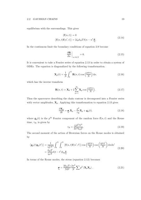
2.2. GAUSSIAN CHAINS 19
equilibrium with the surroundings. This gives
〈f(n, t)〉 = 0
〈
f(n, t)f(n ′ , t) 〉 = 2ζ 0 k B T δ(n − n ′ )I
≈
.
(2.14)
In the continuous limit the boundary conditions of equation 2.9 become
∂R
∂n
⏐ = 0. (2.15)
n=0,N
It is convenient to take a Fourier series of equation 2.13 in order to obtain a system of
ODEs. The equation is diagonalized by the following transformation.
X p (t) = 1 N
∫ N
0
R(n, t) cos
( pπn
)
dn. (2.16)
N
which has the inverse transform
R(n, t) = X 0 + 2
∞∑ ( pπn
)
X p cos . (2.17)
N
p=1
Thus the spacecurve describing the chain contour is decomposed into a Fourier series
with vector amplitudes, X p . Applying this transformation to equation 2.13 gives
∂X p
∂t
= κ
≈
.X p − p2
τ R
X p + g p (t). (2.18)
where g p (t) is the p th Fourier component of the random force f(n, t) and the Rouse
time, τ R , is given by
τ R = ζ 0b 2 N 2
3π 2 k B T . (2.19)
The second moment of the action of Brownian forces on the Rouse modes is obtained
by
〈
gp (t)g q (t ′ ) 〉 = 1
ζ 2 0 N 2 ∫ N
0
∫ N
= k BT
ζ 0 N δ(t − t′ )δ pq I
≈
.
0
〈
f(n, t)f(n ′ , t ′ ) 〉 ( pπn
)
cos cos
N
In terms of the Rouse modes, the stress (equation 2.12) becomes
( qπn
′
N
)
dndn ′
(2.20)
σ = 3k BT c 2π 2 ∑
p 2
≈ Nb 2 〈X p X p 〉 . (2.21)
N