Molecular modelling of entangled polymer fluids under flow The ...

50 CHAPTER 3. THE POM-POM MODEL IN EXPONENTIAL SHEAR.
against experimental data from Zülle et al. (1987), Venerus (2000) and Suneel et al.
(Submitted) using the multimode generalisation [Inkson et al. (1999)] in section 3.3.
3.2 Single mode pom-pom model
Zülle et al. (1987) make a distinction between two types of exponential shear: true
exponential shear as defined in equation 3.1 and nearly exponential shear. Nearly
exponential shear has a shear rate that grows as ˙γ(t) = αe αt . It differs from true
exponential shear by a decaying term of αe −αt and hence the two flows converge when
αt ≫ 1. Note that nearly exponential shear does not have a purely exponential growth
of the extension ratio, except in the limit of long times where the behaviour approaches
true exponential shear. Consequentially the two flows are qualitatively similar and the
data converge for large strains [Zülle et al. (1987)]. In this section the solutions to the
pom-pom equations for nearly exponential shear will be analysed. Since most of this
analysis will be in the t ≫ 1/α limit the results will also hold for true exponential shear.
The solutions to the pom-pom equations for simple shear and planar extension have
been previously studied [see McLeish and Larson (1998), Bishko et al. (1999), Inkson
et al. (1999), Blackwell et al. (2000)]; they will serve as comparisons to the solutions in
exponential shear.
3.2.1 Solutions to the orientation equation
The orientation equation in table 2.2 can be solved analytically for simple shear, nearly
and true exponential shear and planar extension. Throughout the chapter I will be
assume that, for shear flows, the flow is in the x-direction and that the velocity gradient
is in the y-direction. For planar extension the principle stretch will always occur in the
x direction with the z-direction neutral. Simple shear flow is usually described by the
transient stress growth co-efficient, which is defined as η + (t, ˙γ) = σ xy / ˙γ. There is some
ambiguity in the definition of an equivalent material function for exponential shear. In
previous studies a variety of material functions have been used, including dividing the
shear stress by the instantaneous shear rate, ˙γ(t). In this chapter I will simply divide
by the initial shear rate, ˙γ 0 . Note that for true exponential shear ˙γ 0 = 2α and for
nearly exponential shear ˙γ 0 = α
In shear flows the rate at which the flow stretches the backbone segments, κ : S,
≈ ≈
is equal to ˙γS xy . In addition, S xy is also the component of the orientation tensor that
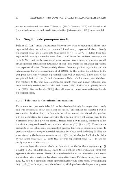
appears in the shear stress. Figure 3.1 shows the solution to the orientation equation for
simple shear with a variety of backbone orientation times. For shear rates greater than
1/τ b , S xy rises to a maximum before approaching its steady state value. By maximising
lim t→∞ S xy (t) with respect to τ b the value of τ b which produces the largest steady state