Agreement DE-FC26-02NT15342, Seismic Evaluation of ...

minimize 1 w
2
2
subject to y
i
− 〈 w x
i
〉 −
⎧
⎨
⎩ 〈 w , x
i
b ≤ ε
〉 + b − y ≤ ε
, (2)
The assumption in (2) was that such a function f actually exists that approximates all
pairs (x i , y i ) with ε precision. If we want to allow for some errors, we may introduce
variables ξ i , ξ * i to arrive at formulation (3):
l
minimize 1 2
*
w + C ∑ ( ξ
i
+ ξ
i
)
2
i = 1
⎧ y
i
− 〈 w,
x
i
〉 − b ≤ ε + ξ
i
subject to
⎪
*
⎨〈
w,
x
i
〉 + b − y
i
≤ ε + ξ
(3)
i
⎪ *
⎩ξ
i
, ξ
i
≥ 0
The constant C > 0 determines the trade-off between the flatness of f and the amount up
to which deviations larger than ε are tolerated. This corresponds to dealing with a so
called ε-insensitive loss function |ξ| ε described by
⎧
= if |ξ| ≤ ε
⎨
⎩ ξ − ε
ξ ε
0 (4)
otherwise.
i
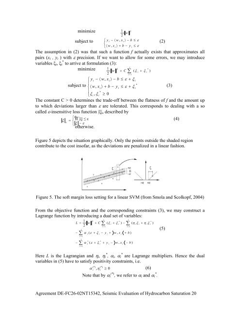
Figure 5 depicts the situation graphically. Only the points outside the shaded region
contribute to the cost insofar, as the deviations are penalized in a linear fashion.
Figure 5. The soft margin loss setting for a linear SVM (from Smola and Scolkopf, 2004)
From the objective function and the corresponding constraints (3), we may construct a
Lagrange function by introducing a dual set of variables:
L =
−
−
l
∑
i = 1
l
∑
i = 1
1
2
w
*
i
2
+ C
*
i
i = 1
α ( ε + ξ − y
i
α ( ε + ξ +
i
l
∑
*
( ξ + ξ ) −
i
y
i
i
+
−
i
w , x
i
w , x
i
l
∑
i = 1
+ b )
− b )
*
( η ξ + η ξ )
Here L is the Lagrangian and η i , η * i , α i , α * i are Lagrange multipliers. Hence the dual
variables in (5) have to satisfy positivity constraints, i.e.
α (*) (*)
i
,η i
≥ 0 (6)
Note that by α i (*) , we refer to α i and α i * .
i
i
i
i
(5)
Agreement DE-FC26-02NT15342, Seismic Evaluation of Hydrocarbon Saturation 20