PDF file - Johannes Kepler University, Linz - JKU

CHAPTER 2. PRELIMINARIES 22
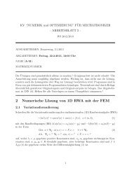
Figure 2.3 A quadrilateral is discretized by decomposition into its sub-triangles.
PSfrag replacements
S 3
S 4
S 5
S 1
S 2
As the midpoint has only connections to S 1 ,. . . ,S 4 — also in the fully assembled matrix
— there would be a line like
a 51 x 1 + a 52 x 2 + a 53 x 3 + a 54 x 4 + a 55 x 5 = f 5
in the system (where x is the solution vector, f the right hand side). Thus we can locally
eliminate the entries for S 5 and get the resulting element matrix
⎛
⎞
a 11 − a 15 a 51 /a 55 a 12 − a 15 a 52 /a 55 −a 15 a 53 /a 55 a 14 − a 15 a 54 /a 55
⎜a 21 − a 25 a 51 /a 55 a 22 − a 25 a 52 /a 55 a 23 − a 25 a 53 /a 55 −a 25 a 54 /a 55
⎟
⎝ −a 35 a 51 /a 55 a 32 − a 35 a 52 /a 55 a 33 − a 35 a 53 /a 55 a 34 − a 35 a 54 /a 55
⎠
a 41 − a 45 a 51 /a 55 −a 45 a 52 /a 55 a 43 − a 45 a 53 /a 55 a 44 − a 45 a 54 /a 55
(and additional right hand side terms if f ≠ 0).
This idea can be generalized to any cell-type (e.g. pentagons, pyramids, hexahedra,
octahedra, or prisms). First, one has to split the cell into triangles resp. tetrahedra and
then eliminate the auxiliary unknowns locally.
2.3 The Non-Stationary Problem
In the non-stationary case we use the method of lines for time integration. First, the weak
formulation and the FEM approximation in the space variables (with time dependent
coefficients) is performed as shown above to get the system
d
dt (u h, v h ) 0 + a D (u h , v h ) + a C (u h ; u h , v h ) + b(v h , p h ) = 〈F, v h 〉 ,
b(u h , q h ) = 0
(plus initial conditions), a system of ordinary differential equations, where standard methods
of time integration can be applied [HWN00].
To show two examples thereof, we assume that the k-th time step has length δ k and
that the right hand side is constant in time, and we search the discrete solution (u k , p k ) at
time t k = t 0 + ∑ k
i=1 δ i.