PDF file - Johannes Kepler University, Linz - JKU

CHAPTER 3. MULTIGRID METHODS 36
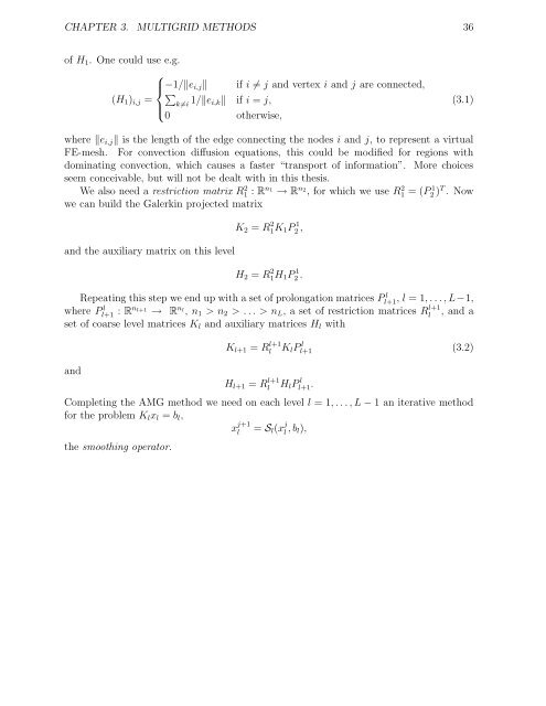
of H 1 . One could use e.g.
⎧
⎪⎨ −1/‖e i,j ‖ if i ≠ j and vertex i and j are connected,
∑
(H 1 ) i,j =
k≠i
⎪⎩
1/‖e i,k‖ if i = j,
0 otherwise,
(3.1)
where ‖e i,j ‖ is the length of the edge connecting the nodes i and j, to represent a virtual
FE-mesh. For convection diffusion equations, this could be modified for regions with
dominating convection, which causes a faster “transport of information”. More choices
seem conceivable, but will not be dealt with in this thesis.
We also need a restriction matrix R1 2 : R n 1
→ R n 2
, for which we use R1 2 = (P2 1 ) T . Now
we can build the Galerkin projected matrix
and the auxiliary matrix on this level
K 2 = R 2 1 K 1P 1 2 ,
H 2 = R 2 1 H 1P 1 2 .
Repeating this step we end up with a set of prolongation matrices Pl+1 l , l = 1, . . . , L−1,
where Pl+1 l : Rn l+1 → R
n l, n1 > n 2 > . . . > n L , a set of restriction matrices R l+1
l
, and a
set of coarse level matrices K l and auxiliary matrices H l with
and
K l+1 = R l+1
l
K l Pl+1 l
(3.2)
H l+1 = R l+1
l
H l Pl+1 l .
Completing the AMG method we need on each level l = 1, . . . , L − 1 an iterative method
for the problem K l x l = b l ,
= S l (x j l , b l),
the smoothing operator.
x j+1
l