PDF file - Johannes Kepler University, Linz - JKU

CHAPTER 3. MULTIGRID METHODS 40
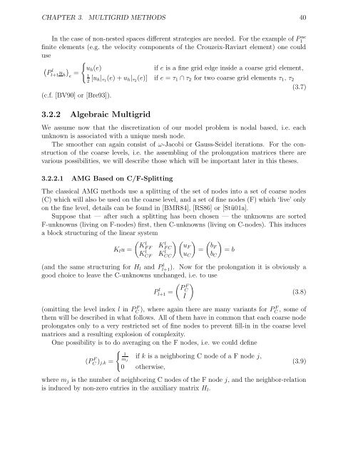
In the case of non-nested spaces different strategies are needed. For the example of P1
nc
finite elements (e.g. the velocity components of the Crouzeix-Raviart element) one could
use
{
( )
P
l
l+1 u = u h (e)
if e is a fine grid edge inside a coarse grid element,
h e 1
[u 2 h| τ1 (e) + u h | τ2 (e)] if e = τ 1 ∩ τ 2 for two coarse grid elements τ 1 , τ 2
(3.7)
(c.f. [BV90] or [Bre93]).
3.2.2 Algebraic Multigrid
We assume now that the discretization of our model problem is nodal based, i.e. each
unknown is associated with a unique mesh node.
The smoother can again consist of ω-Jacobi or Gauss-Seidel iterations. For the construction
of the coarse levels, i.e. the assembling of the prolongation matrices there are
various possibilities, we will describe those which will be important later in this theses.
3.2.2.1 AMG Based on C/F-Splitting
The classical AMG methods use a splitting of the set of nodes into a set of coarse nodes
(C) which will also be used on the coarse level, and a set of fine nodes (F) which ‘live’ only
on the fine level, details can be found in [BMR84], [RS86] or [Stü01a].
Suppose that — after such a splitting has been chosen — the unknowns are sorted
F-unknowns (living on F-nodes) first, then C-unknowns (living on C-nodes). This induces
a block structuring of the linear system
(
K
l
K l u = F F KF l C
KCF
l KCC
l
) ( )
uF
=
u C
(
bF
)
= b
b C
(and the same structuring for H l and Pl+1 l ). Now for the prolongation it is obviously a
good choice to leave the C-unknowns unchanged, i.e. to use
( ) P
Pl+1 l = F
CI (3.8)
(omitting the level index l in PC F ), where again there are many variants for P C F , some of
them will be described in what follows. All of them have in common that each coarse node
prolongates only to a very restricted set of fine nodes to prevent fill-in in the coarse level
matrices and a resulting explosion of complexity.
One possibility is to do averaging on the F nodes, i.e. we could define
{
1
(PC F ) m
j,k = j
if k is a neighboring C node of a F node j,
(3.9)
0 otherwise,
where m j is the number of neighboring C nodes of the F node j, and the neighbor-relation
is induced by non-zero entries in the auxiliary matrix H l .