Computational Models of Music Similarity and their ... - OFAI
Computational Models of Music Similarity and their ... - OFAI
Computational Models of Music Similarity and their ... - OFAI

Create successful ePaper yourself
Turn your PDF publications into a flip-book with our unique Google optimized e-Paper software.
34 2 Audio-based <strong>Similarity</strong> Measures<br />
Blue Rondo A La Turk<br />
86.4<br />
Kathy’s Waltz<br />
80.9<br />
Bad Medicine<br />
38.6<br />
10<br />
20<br />
30<br />
0<br />
−39.5<br />
0<br />
−28.4<br />
0<br />
−9.1<br />
Bring Me To Life<br />
37.4<br />
Someday<br />
85.1<br />
Bolero<br />
43.0<br />
10<br />
20<br />
30<br />
10 20 30<br />
0<br />
−13.3<br />
10 20 30<br />
0<br />
−13.6<br />
10 20 30<br />
0<br />
−13.7<br />
Figure 2.12: Full covariance matrices for 6 songs (G1). On both axes the dimensions<br />
are Mel frequency b<strong>and</strong>s. The dimension <strong>of</strong> the gray shadings is dB.<br />
the problem pieces had only little variance in <strong>their</strong> spectra. For example,<br />
one <strong>of</strong> them was very short (30 second) <strong>and</strong> calm. Such cases can easily be<br />
identified <strong>and</strong> excluded (e.g., all pieces can be ignored which have a value<br />
larger than 10 10 in the inverse covariance).<br />
Illustrations<br />
Figure 2.12 shows the covariances for the 6 songs used in previous figures. As<br />
can be seen, there is a lot <strong>of</strong> information besides the diagonal. Noticeable are<br />
that the variances for lower frequencies are higher. Furthermore, for some<br />
<strong>of</strong> the songs there is a negative covariance between low frequencies <strong>and</strong> mid<br />
frequencies.<br />
Figure 2.13 shows the same plots for G1 which were already discussed for<br />
G30 <strong>and</strong> G30S in Figures 2.10 <strong>and</strong> 2.11. Since G1 uses only one Gaussian,<br />
there is only one line plotted in the second row. Noticeable, is also that there<br />
are more lines visible in rows 4 <strong>and</strong> 5. This indicates there are fewer frames<br />
(sampled or original) which have much higher probabilities than all others.<br />
Otherwise, in particular the third <strong>and</strong> last row are very similar to those <strong>of</strong><br />
G30 <strong>and</strong> G30S <strong>and</strong> indicate that the models are very similar.<br />
2.2.3.5 Computation Times<br />
The CPU times for G30, G30S, <strong>and</strong> G1 are given in Table 2.1. The frame<br />
clustering (FC) time is less interesting than the time needed to compute the<br />
cluster model similarity (CMS). While FC can be computed <strong>of</strong>fline, either all<br />
possible distances need to be precomputed (<strong>and</strong> at least partially stored) or