Lecture 9: Linear Programming

Lecture 9: Linear Programming 

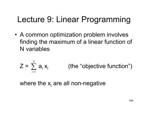
• A common optimization problem involves 

finding the maximum of a linear function of 

N variables 

N 

Z = ∑ a i x i 

i= 

1 

(the “objective function”) 

where the x i are all non-negative 

194

Linear Programming 

….subject to a series of M constraints 

N 

∑ 

i= 

1 

≤ 

c ij x i = b j j = 1, 2, 3, …,M 

≥ 

where the b j are all non-negative 

195

Linear Programming 

• The constraints are each represented by N–1 

dimensional hyperplanes within the N-dim space 

– these form a convex hyperpolygon in N dimensions 

bounding a region of volume V N 

–if V N is zero (all volume eliminated), there is no 

solution 

–if V N is > 0, then the gradient ∇Z = a i e i 

to a boundary plane 

∑ 

i= 

1 

leads us 

• Unless ∇Z is perpendicular to the boundary plane, we can 

follow that plane to an edge and that edge to a vertex a 

single optimal vector 

N 

196

Feasible vectors 

• The space of vectors satisfying the constraints is called 

the space of “feasible vectors”, and the vertex that 

maximizes Z is the “optimal feasible vector” 

• Vertices of the hyperpolygon are places that satisfy N 

constraints as equalities: these are called basic feasible 

vectors. (Here, the “constraints” include the nonnegativity 

requirement on the x i ). 

197

Feasible vectors 

• 2-D example: Z = x 1 + x 2 

x 1 

x 2 

x 2 – x 1 < 1 

Optimal feasible vector 

x 1 < 3 

Feasible basic vector 

x 1 + 2x 2 

< 4 

∇Z 

Space of 

feasible vectors 

198

The fundamental theorem of 

linear programming 

“If an optimal feasible vector exists, then 

there is a feasible basic vector that is 

optimal” 

i.e. the optimal vector is at one of the vertices 

Our goal is to find which vertex (i.e. which N of 

the constraints does it satisfy) 

199

Feasible basic vectors 

The total number of locations at which N constraints are 

satisfied simultaneously can be very large: 

It can be as large as the number of ways of choose N items 

out of N+M, which comes to (N+M)! / (N! M!) 

In the 2-D example, N=2, M=3, and so 

(N+M)! / (N! M!) = 5!/(3!2!) = 10 

of which 5 lie in the feasible space and one is missing 

(since x 1 =0 and x 1 =3 cannot be satisfied simultaneously) 

200

Restricted normal form 

• The constraints can always be written 

such that 

– All constraints are written as equalities 

– Number of constraints M ≤ N 

– Each constraint equation has a variable that 

appears in that equation alone 

(How to do this to be discussed later) 

• This permits us to obtain a solution via the 

“simplex method” 

201

The simplex method 

(illustrated by example) 

• Example (N=4, M=2) 

Maximize z = – 4x 1 – 25x 2 + 4x 3 + x 4 

subject to x 1 + 6x 2 –x 3 = 2 

–3x 2 + 4x 3 + x 4 = 8 

Move variables that appear in only one 

constraint equation to the left hand side and call 

them left hand variables 

202

Solution via the simplex method 

This yields x 1 = 2 – 6x 2 + x 3 

x 4 = 8 + 3x 2 –4x 3 

which we substitute into the objective 

function to obtain the latter in terms of 

right hand variables 

z = 2x 2 –4x 3 

There are M left hand variables and N – M 

right hand variables 

203


Represent these equations by a “tableau”: 

z = 2x 2 –4x 3 

x 1 = 2 – 6x 2 + x 3 

x 4 = 8 + 3x 2 –4x 3 

is written 

const 

x 2 x 3 

z 0 + 2 –4 

x 1 + 2 –6 + 1 

x 4 + 8 + 3 –2 

204


Setting the RH variables equal to zero, we can immediately 

obtain a basic feasible vector (but not, in general, the 

optimal one) x = (+2, 0, 0, +8) 

Increasing x 3 from zero will clearly decrease z, so we 

conclude that the optimal feasible vector must have x 3 = 0 

const 

x 2 x 3 

z 0 + 2 –4 

x 1 + 2 –6 + 1 

x 4 + 8 + 3 –2 

205


We now “pivot” about the negative entry that limits how 

large x 2 can become, and switch the “handedness” of x 1 

and x 2 . 

x 1 = 2 – 6x 2 + x 3 x 2 = 1/3 – x 1 /6 + x 3 /6 

x 4 = 8 + 3x 2 –4x x 3 4 = 8 + 3(1/3 – x 1 /6 + x 3 /6) – 4x 3 

= 9 – x 1 /2 – 7x 3 /2 

z = 2x 2 –4x 3 z = 2(1/3 – x 1 /6 + x 3 /6) – 4x 3 

= 2/3 – x 1 /3 – 11x 3 /3 

206


Our new LH variables are x 1 and x 3 and our new RH 

variables are x 4 and x 1 

And our new tableau is 

const 

x 1 x 3 

z +2/3 –1/3 – 11/3 

x 2 +1/3 –1/6 + 1/6 

x 4 + 9 –1/2 –7/2 

207


Setting the RH variables to zero, we find that the feasible 

basic vector we can immediately write is now 

x = (0 ,+1/3, 0, +9), for which z = 2/3 

Because all the entries in the z-row are now negative, this 

is the optimum feasible vector, because increasing either 

RH variable will only decrease z 

const 

x 1 

x 3 

z + 2/3 –1/3 – 11/3 

x 2 + 1/3 –1/6 + 1/6 

x 4 + 9 –1/2 –7/2 

208

Generalization to N variables 

and M constraints 

const 

z 

> 0 

< 0 

< 0 

> 0 

< 0 

< 0 

“z-row” 

< 0 

M 

< 0 

< 0 

Pivot has largest 

ratio of –value/const 

N – M 

209

Keep pivoting until the “z row” 

is all negative 

Zero components 

of optimal feasible vector 

const 

z 

< 0 

< 0 

< 0 

< 0 

< 0 

< 0 

M 

Maximum value of z 

Non-zero components 

of optimal feasible vector 

their values 

N – M 

210

Generalization to N variables 

and M constraints 

• The maximum number of required pivots is 

min(N – M, M) 

• The process can (and should) fail if there 

are no negative entries in a column 

headed by a positive pivot 

– implies there is no maximum allowed 

value of z (i.e. no boundary prevents us 

from going to infinity along that basis 

vector) 

211

Obtaining the constraints in 

restricted normal form 

• What happens if 

– Some constraints are inequalities 

– Not every constraint equation has a variable 

that appears in that equation alone 

– Number of constraints M > N 

• General solution: increase the number of 

variables! 

212

Treatment of inequalities 

Suppose we want 

N 

∑ 

i= 

1 

c ij x i ≤ b j for one particular j 

Introduce new non-negative variable, y j , (called a 

“slack variable”), and consider the constraint 

N 

∑ 

i= 

1 

c ij x i + y j = b j 

213


(Equivalently, for 

N 

∑ 

i= 

1 

c ij x i ≥ b j for one or more j 

we use the constraint 

N 

∑ 

i= 

1 

c ij x i –y j = b j ) 

214


• Convert all inequalities according to this 

prescription 

– This increases the dimensionality of the 

problem from N to N + K, where K is the 

number of inequalities 

– Solve by the previous method 

– Ignore the solution for the y j 

215

Getting the constraints into 


Arranging for every constraint equation to 

have a variable that appears in that equation 

alone 

Change the constraint equations into “zero 

form”: 

Define z j ≡ ∑ c ij x i – b j 

N 

i= 

1 

The original M constraints become z j = 0 

216



M 

∑ 

First use Z′ = – z j as the “auxiliary” objective 

function 

j= 

1 

And adopt the definitions of the z j as the M constraints. 

Initially, the z j are all LH variables and the x i are all RH 

variables. This is a problem in restricted normal form 

The solution which maximizes Z′ has all the z i equal to 

zero* after the Simplex method is done, all the z j must 

become RH variables, and M out of N the x i will be LH 

variables. 

*if such a solution exists: if not, then the constraints cannot 

be satisfied simultaneously 

217



But now each of the RH variables appears in 

exactly 1 constraint equation. We zero out 

all the z j , and have a problem involving the x i 

in restricted normal form. 

This we now solve via the Simplex method, 

using the original objective function 

N 

Z = ∑ a i x i 

i= 

1 

218

What if the number of constraints 

exceeds the number of variables? 

If M > N, we can’t possibly have a restricted 

normal form (there aren’t enough variables for 

each constraint to have a variable that appears in 

that constraint alone). 

But the method described above adds M more 

variables, so the number of variables always 

exceeds the number of constraints. 

219

Lecture 9: Linear Programming

Create successful ePaper yourself

Delete template?

Save as template?