1.Pendulum
1.Pendulum
1.Pendulum

Create successful ePaper yourself
Turn your PDF publications into a flip-book with our unique Google optimized e-Paper software.
first name (print) last name (print) Brock ID (ab13cd) TA initials grade<br />
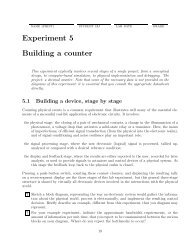
Experiment 1<br />
The pendulum<br />
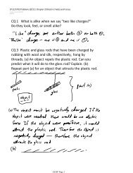
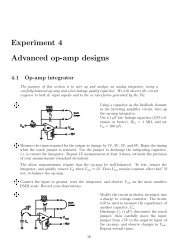
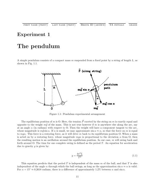
A simple pendulum consists of a compact mass m suspended from a fixed point by a string of length L, as<br />
shown in Fig. 1.1.<br />
Figure 1.1: Pendulum experimental arrangement<br />
The equilibrium position of m is O. Here, the tension ⃗P exerted by the string on m is exactly equal and<br />
opposite to the weight m⃗g of the mass. This is not true however if m is anywhere else along the arc, say<br />
at an angle α (in radians) with respect to O. Then the weight will have a component tangent to the arc,<br />
whose magnitude is m⃗gsinα. If α is small, we may approximate sinα ≈ α, so that the force on m is equal<br />
to mgα. This force is a restoring force, as it will drive m back to its equilibrium position O. When a mass<br />
is acted on by a restoring force, whose magnitude mgα is proportional to the deviation α from O, then<br />
the resulting motion is an oscillation around the equilibrium position. In our case, m will swing back and<br />
forth around O. The time for one complete swing is defined as the period T. An equation for acceleration<br />
due to gravity g is given by:<br />
g = 4π2 L<br />
T 2 (1.1)<br />
This equation predicts that the period T is independent of the mass m of the ball, and that T is also<br />
independent of the angle α through which the ball swings, as long as the approximation sinα ≈ α is valid.<br />
For α = 15 ◦ ≈ 0.2618 radians, there is a difference of approximately 1.2% between α and sinα.<br />
11
12 EXPERIMENT 1. THE PENDULUM<br />
Introduction to error analysis<br />
The result of a measurement of a physical quantity must contain not only a numerical value expressed in<br />
the appropriate units; it must also indicate the reliability of the result. Every measurement is somewhat<br />
uncertain. Error analysis is a procedure which estimates quantitatively the uncertainty in a result. This<br />
quantitative estimate is called the error of the result. Please note that error in this sense is not the same as<br />
mistake. Also, it is not the difference between a value measured by you and the value given in a textbook.<br />
Error is a measure of the quality of the data that your experiment was able to produce. In this lab, error<br />
will be considered a number, in the same units as the result, which tells us the precision, or reliability,<br />
of that experimental result. Note that error value, represented by the Greek letter σ (sigma), is always<br />
rounded to one significant digit; the result is always rounded to the same decimal place as σ (see below).<br />
Error of a single measurement<br />
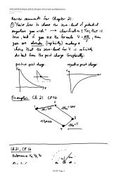
Consider the measurement of the length L of a bar<br />
using a metre stick, as shown in Figure 1. One can<br />
see that L is slightly greater than 2.1 cm, but because<br />
the smallest unit on the metre stick is 1 mm,<br />
it is not possible to state the exact value. We can,<br />
however, safely say that L lies between 2.1 cm and<br />
2.2 cm. The proper way to express this information<br />
is:<br />
L±σ(L) = 2.15±0.05 cm<br />
This expression states that L must be between,<br />
(2.15−0.05) = 2.10cmand, (2.15+0.05) = 2.20cm,<br />
Figure 1.2: Measurement with a metre stick which is our observation. The quantity σ(L) =<br />
±0.05 cm is referred to as the maximum error. This<br />
number gives the maximum range over which the correct value for a measurement might vary from that<br />
recorded, and represents the precision of the measuring instrument.<br />
Propagation of errors<br />
In many experiments the desired quantity, call it Z, is not measured directly, but is computed from one<br />
or more directly-measured quantities A,B,C,... with a mathematical formula. In this experiment, the<br />
directly-measured quantities are T, y and b, and the desired quantity g is calculated from g = 4π 2 L/T 2 ,<br />
with L = y + 1 2b. The following rules give a quick (but not exact) estimate of σ(Z) if σ(A), σ(B) etc.<br />
are known Always use the absolute value of an error in a calculation . Error rules are tabulated in the<br />
Appendix.<br />
1. If Z = cA, where c is a constant, then σ(Z) = |c|σ(A). This is used only if A is a single term. For<br />
example, it can be used for Z = 3y, so that σ(Z) = 3σ(y), but not for Z = 3xy.<br />
2. If Z = A+B +C +···, then σ(Z) = σ(A)+σ(B)+σ(C)+···. For example, if<br />
L = y + 1 2 b<br />
then σ(L) = σ(y)+σ<br />
( 1<br />
2 b )<br />
(See 2. above.)<br />
σ(L) = σ(y)+ 1 σ(b) (See 1. above.)<br />
2
13<br />
3. To derive an error equation for any relation, rewrite that relation as a series of multiplications, then<br />
apply the change of variables method as shown in the Appendix to evaluate the error terms:<br />
g = 4π2 L<br />
T 2 −→ g = 4π 2 LT −2 −→ g = ABCD, ( letting A = 4, B = B = π 2 , C = L, D = T −2 )<br />
Then<br />
and σ(A) = σ(4),<br />
σ(g)<br />
|g|<br />
σ(B)<br />
|B|<br />
= σ(A) + σ(B)<br />
|A| |B|<br />
( σ(π)<br />
= |2|<br />
|π|<br />
+ σ(C)<br />
|C|<br />
)<br />
, σ(C) = σ(L),<br />
+ σ(D) , (Appendix, Rule 4)<br />
|D|<br />
σ(D)<br />
|D|<br />
= |−2|<br />
( ) σ(T)<br />
. (Rules 1,6)<br />
|T|<br />
Thequantities 4 and π are constants and have no error (strictly speaking, σ(4) = σ(π) = 0), therefore<br />
these terms do not contribute to the overall error. The error equation for g then simplifies to<br />
σ(g)<br />
= σ(4) ( ) σ(π)<br />
+2 + σ(L) ( ) σ(T)<br />
+|−2| −→<br />
σ(g) = σ(L) ( ) σ(T)<br />
+2 .<br />
|g| |4| |π| |L| |T| |g| |L| |T|<br />
The right hand side of the above equation, called the “relative error” of g, results in a fraction that<br />
describes how large σ(g) is with respect to g. The desired quantity, σ(g), is obtained by multiplying<br />
both sides of the equation by g:<br />
[ ( )] σ(L) σ(T)<br />
σ(g) = |g| +2 .<br />
|L| |T|<br />
Standard deviation of a series of measurements<br />
When the same measurement or calculation is repeated several times, an error estimate can be calculated<br />
form the variation in this set of values. This is convenient because on other error values, measured or<br />
calculated, need to be known. For example, the five results for g can be used to estimate an error σ(g).<br />
To calculate the standard deviation σ(g) for a sample of N values of g:<br />
1. determine the average 〈g〉 of N values g i , where i = 1,2,···,N by summing the values and then<br />
dividing by the number of values:<br />
〈g〉 = 1 N (g 1 +g 2 +···+g N );<br />
2. for each g i , calculate the deviation ∆g i = g i −〈g〉 from the average 〈g〉;<br />
3. for each g i , calculate the square of the deviation (∆g i ) 2 to make all the values positive;<br />
4. calculate the variance σ 2 (g) of the sample by summing the squares of the deviations (∆g i ) 2 and<br />
dividing by the number of values minus one, N −1<br />
σ 2 (g) = 1<br />
N −1 (∆g2 1 +∆g 2 2 +···+∆g 2 N);<br />
5. undo the previous squaring operation by taking the square root of the variance. This is the root<br />
average squared deviation, or standard deviation σ(g), of b:<br />
√<br />
σ(g) = σ 2 (g)<br />
A large σ value indicates a result which is not very precise. The theory of statistics shows that the<br />
probability that a further measurement of g falls within the range of σ(g) is 68% and that σ is proportional<br />
to 1/ √ N, so σ will decrease as the number of samples N is increased.
14 EXPERIMENT 1. THE PENDULUM<br />
Rounding a final result: X ±σ(X)<br />
The value of σ(x) is rounded to one significant digit whether it represents a maximum error estimate,<br />
calculated error, or standard deviation of a sample. The result correspondingto this error must be rounded<br />
off and expressed to the same decimal place as the error. For example, 〈x〉 = 25.344 mm and σ(x) =<br />
0.0427 mm. Rounded to one digit, σ(x) = 0.04 mm. Rounded to the same decimal place, 〈x〉 = 25.34 mm.<br />
The final result is expresses as 〈x〉±σ(x) = (25.34 ± 0.04) mm.<br />
Do not use a rounded off value in further calculations. Use the original unrounded value. Use of a<br />
truncated value will decrease the quality of your result.<br />
Powers of 10<br />
Express both the result and its error to the same power of 10. This allows the reader to immediately judge<br />
how large the error is relative to the result:<br />
1. 2.68 × 10 −2 ± 5 × 10 −4 should be written as 0.0268 ± 0.0005 or (2.68 ± 0.05) × 10 −2 . Note the<br />
parentheses, indicating that both the result and the error are to be multiplied by 10 −2 .<br />
2. 1.634±3×10 −3 m should be written as 1.634±0.003 m<br />
Format of calculations<br />
Record all calculations, in the appropriate space if provided or on a separate sheet of paper. A calculation<br />
is performed in three lines. The first line displays the formula used. In the second line, the variables in the<br />
formula are replaced with the actual values used in the calculation. The third line shows the final answer<br />
formatted according to the section on Rounding above and if any, the units associated with the result.<br />
Review questions<br />
Using a textbook, the Physics Handbook, the Internet or some other source, find the accepted value of g.<br />
Cite your reference so that a reader can find this information. Be specific; do not cite ’my physics book’,<br />
’my buddy’ or ’i remember it from high school’ as your source. Include specific info such as the uncertainty,<br />
or error, in the value, and the condition (i.e. sea level) under which it was measured.<br />
g = ..............................................................................<br />
An error value is only meaningful when expressed with ..... significant digits.<br />
The measurement error σ of a scale graduated in minutes and seconds is ....................<br />
My Lab dates: Exp.1:...... Exp.3:...... Exp.4:...... Exp.5:...... Exp.6......<br />
I have read and understand the contents of the Lab Outline (sign) ................<br />
CONGRATULATIONS! YOU ARE NOW READY TO PROCEED WITH THE EXPERIMENT!<br />
Procedure and analysis<br />
You will determine theperiodT of a pendulumof length L by monitoringthe distance of thependulumbob<br />
from a computer controlled rangefinder. This device determines the distance to an object by transmitting<br />
an untrasonic ping and measuring the time required to receive the echo of the original signal after it is<br />
reflected from the object.
15<br />
The transmitted signal propagates in a narrow conical beam and as it is the echo from the nearest<br />
object that is accepted, you will need to be sure that you are pinging the pendulum bob and not the<br />
pendulum arm or some other structure in the cone of the beam. As the pendulum bob swings toward and<br />
away from the rangefinder, the variation in distance over time can be approximated by a sine wave. By<br />
analysing the properties of this sine wave, we can calculate the period T of the pendulum.<br />
The pendulum is an aluminum ball suspended by a light nylon string from a sliding arm. Assume the<br />
mass of the string is negligibly small compared to the mass of the ball. To calibrate the pendulum:<br />
1. Release the string to set the ball on the table. Align the bottom of the sliding arm with the zero<br />
mark on the scale. Adjust the string length so that the top of the ball lightly contacts the bottom of<br />
the arm, ensuring that the string is not stretched. Secure the string with the clamping nut.<br />
2. Raise the arm away from the ball and carefully reposition the arm until it once again just contacts<br />
the top of the ball. If the bottom of the arm is no longer at the zero mark, repeat the sequence of<br />
adjustments until the bottom of the arm is in line with the zero mark of the scale and the arm lightly<br />
contacts the top of the pendulum ball. All members of the group must check the calibration.<br />
The scale is now calibrated to display the length of the string y from the bottom of the sliding arm,<br />
the pivot point of the pendulum, to the top of the ball, to a precision of one millimetre (mm). This<br />
number is not exactly equal to L since the ball is not a point-mass. The length of the pendulum L is the<br />
sum of the length of the string y and half the ball’s diameter b given in Table 1.1:<br />
L = y + 1 b. (1.2)<br />
2<br />
Mount the larger ball m 1 and calibrate the pendulum. Adjust the sliding arm so that the string length<br />
y is approximately 0.3 m. Record the actual length to a precision of 1 mm.<br />
• Set the pendulum swinging in a straight line, keeping α less than approximately 15 ◦ . Wait several<br />
seconds to allow for any stray oscillations present in the bob to dissipate.<br />
• Shift focus to the Physicalab software. Check the Dig1 box and choose to collect 50 points at 0.1<br />
s/point. Click Get data to acquire a data set.<br />
• Click Draw to generate a graph of your data. Your points should display a nice smooth sine<br />
wave, without peaks, stray points, or flat spots. If any of these are noted, adjust the position of the<br />
rangefinder and acquire a new data set.<br />
• Select fit to: y= and enter A*sin(B*x+C)+D in the fitting equation box. Click Draw . If<br />
you get an error message the initial guesses for the fitting parameters may be too distant from the<br />
required values for the fitting program to properly converge. Look at your graph and enter some<br />
reasonable initial values for the amplitude A of the wave and the average distance D of the wave<br />
from the detector. The value of B (in radians/s) is given by B = 2π/T since the period of a sine<br />
wave is 2π = B∗x radians, where x = T is the period in seconds. Estimate the time T between two<br />
adjacent minima of the sine wave. Estimate and enter an initial guess for B. (See Appendix A)<br />
• Label the axes and identify the graph with your name and the string length y used. Click Print<br />
to print your graph. Every student should print a copy of each graph.<br />
• Record in Table 1.1 the trial length y and the computer calculated value of the fitting parameter B<br />
(radians/second). Do a quick calculation for g to make sure that the value is reasonable.<br />
• Repeat the above steps for m 1 with y = 0.45, 0.60, 0.75 and 0.90 m.<br />
• Mount the second ball m 2 , recalibrate the pendulum and verify the calibration, set the string<br />
length to approximately y = 0.5 m, and record this one measurement in Table 1.1.
16 EXPERIMENT 1. THE PENDULUM<br />
Run, i m (kg) b (m) y (m) L (m) B (rad/s) T (s) T 2 (s 2 ) g i (m/s 2 )<br />
1,m 1 0.0225 0.02540<br />
2,m 1 0.0225 0.02540<br />
3,m 1 0.0225 0.02540<br />
4,m 1 0.0225 0.02540<br />
5,m 1 0.0225 0.02540<br />
1,m 2 0.0095 0.01904<br />
Table 1.1: Table of experimental results<br />
Part I: Determining g from a single measurement<br />
• Use Equation 1.2 and the single measurement of m 2 to calculate L and g. Show the calculation<br />
below, in three steps as previously outlined and recalling the proper application of significant figures<br />
and physical units.<br />
L = ............................... g = ...............................<br />
............................... ...............................<br />
............................... ...............................<br />
• The measurement errors in y, b, and T, represented by σ(y), σ(b), and σ(T), respectively, are<br />
determined from the scales of the measuring instruments. The micrometer used to measure the ball<br />
has a resolution, or scale increment of 0.00001 m. The data logger can measure time with a precision<br />
of 0.00002 s. Summarize these measurement errors below:<br />
σ(y) = ±.................. σ(b) = ±.................. σ(T) = ±..................<br />
• Calculate the error σ(L) in the length L and the error σ(g) in g. Express the final values as L±σ(L)<br />
and as g±σ(g), with the correct units.<br />
σ(L) = ............................... σ(g) = ...............................<br />
............................... ...............................<br />
............................... ...............................<br />
L = ..............±............... g = ..............±...............
17<br />
Part II: Determining g from a series of measurements<br />
• Use Equation 1.1 to calculate the five measurements of g for m 1 . Record the results in Table 1.1 and<br />
Table 1.2. Include all the calculations for m 1 as part of your Lab Report.<br />
• Use Table 1.2 to calculate the average and standard deviation of the sample of g values, then summarize<br />
the result in the proper format below:<br />
i g i g i −〈g〉 (g i −〈g〉) 2<br />
1<br />
2<br />
3<br />
4<br />
5<br />
〈g〉 = variance =<br />
σ(g) =<br />
Table 1.2: Calculation template for the standard deviation of g.<br />
g = .............±.............<br />
Part III: Determining g from the slope of a graph<br />
Equation 1.1 can be written as:<br />
L =<br />
( g<br />
4π 2 )<br />
T 2 (1.3)<br />
This is the equation of a straight line Y = mX + b, where in this case Y = L, X = T 2 , b = 0, and the<br />
slope m = rise/run = g/(4π 2 ).<br />
• Using the Physica Online software, enter the five coordinates (T 2 ,L) in the data window. Select<br />
scatter plot. Click Draw to generate a graph of your data. Select fit to: y= and enter A*x+B<br />
in the fitting equation box. Click Draw . The computer will generate a line of best fit through the<br />
data points. Print the graph, then record below the slope A and error σ(A)<br />
• Calculate below values for g and σ(g).<br />
A = .............±.............<br />
g = ....................... = ....................... = .......................<br />
σ(g) = ....................... = ....................... = .......................<br />
g = .............±.............
18 EXPERIMENT 1. THE PENDULUM<br />
Summary of results<br />
Nowthatyouhavequantitatively estimatedthereliability ofyourvariousresultsforg byapplicationoferror<br />
analysis, you can make a meaningful comparison of these results with the accepted value of g = 9.80 m/s 2 .<br />
• In the space below, plot and label your three results for g and the error bars representing the<br />
uncertainty in each of these results. Begin by drawing on the given line a scale that is representative<br />
of the range in your results. The range of agreement in two results is determined by the region of<br />
overlap of their error bars. For clarity, plot your data and error bars above one another.<br />
• Which of the error bars overlap the accepted value of g? ...............................<br />
• Is there a region where all the error bars overlap? .....................................<br />
• Do any of your error bars overlap the accepted value of g? ..............................<br />
IMPORTANT: BEFORE LEAVING THE LAB, HAVE A T.A. INITIAL YOUR WORKBOOK!<br />
Discussion<br />
Your Discussion should summarize the essence of this experiment in a clear and organized way, so that<br />
someone reading (or marking) this report will obtain a good understanding of what was done, how it was<br />
done, and of the results that were obtained. Here are some ideas on the issues you should address in your<br />
discussion:<br />
Begin by tabulating your three experimental values and the accepted value of g. Identify the source of<br />
the data and include appropriate units. Give the table a descriptive title.<br />
Compare your three results for g. Do your values agree with the accepted value of g. Explain your<br />
reasoning.<br />
Consider which method is likely to provide the most reliable value for g. Which method is the least<br />
reliable? Explain your conclusions.<br />
From your graph, determine whether T varies with L. Does T vary with the mass of the ball? Explain.<br />
Do your conclusions agree with the predictions of Equation 1.1?<br />
Both the averaging method and the line of best fit use the same five experimental values for L and T.<br />
What similarities do you think there may be in these two approaches to determining g?<br />
If drawing a line through the plotted experimental points, how would you choose where to place the<br />
line? How might this choice affect your resulting value of g?<br />
What is the resolution, or scale, of the time measurement and how did you determine this? How might<br />
the resolution be improved?<br />
A Final Note: Have you printed and included the complete email that Turnitin sent you<br />
containing the full content of your Discussion? If not, you will lose 40% of your grade. Printouts of the<br />
receipt from the Turnitin webpage or your wordprocessor will not be considered for marking.