Brock University Physics Department PHYS 1P92 Laboratory Manual
Brock University Physics Department PHYS 1P92 Laboratory Manual
Brock University Physics Department PHYS 1P92 Laboratory Manual

You also want an ePaper? Increase the reach of your titles
YUMPU automatically turns print PDFs into web optimized ePapers that Google loves.
<strong>Brock</strong> <strong>University</strong> <strong>Physics</strong> <strong>Department</strong><br />
St. Catharines, Ontario, Canada L2S 3A1<br />
<strong>PHYS</strong> <strong>1P92</strong> <strong>Laboratory</strong> <strong>Manual</strong><br />
<strong>Physics</strong> <strong>Department</strong><br />
Copyright c○ <strong>Brock</strong> <strong>University</strong>, 2012-2013
Contents<br />
<strong>Laboratory</strong> rules and procedures 1<br />
Introduction to Physica Online 5<br />
1 Capacitance 11<br />
2 Check your schedule! 21<br />
3 Faraday rotation 23<br />
4 Resistance 31<br />
5 Electron charge-to-mass ratio 41<br />
6 Diffraction of light by a grating 49<br />
A Review of math basics 57<br />
B Error propagation rules 59<br />
C Graphing techniques 61<br />
i
<strong>Laboratory</strong> rules and procedures<br />
<strong>Physics</strong> <strong>Department</strong> lab instructors<br />
Frank Benko, office B210a, ext.3417, fabenko@brocku.ca<br />
Phil Boseglav, office B211, ext.4109, fbosegla@brocku.ca<br />
This information is important to YOU, please read and remember it!<br />
<strong>Laboratory</strong> schedule<br />
To determine your lab schedule, click on the marks link in your course homepage; your lab dates are<br />
shown in place of the lab marks and correpond to the section number that you selected when you registered<br />
for the course. You cannot change these dates unless you have a conflict with another course and make<br />
the request in writing.<br />
The schedule consists of five Experiments to be performed every second week on the same<br />
weekday. On any given day there are four different Experiments taking place, with up to three groups<br />
of no more than two students in a group performing the same experiment. You need to:<br />
• prepare for your scheduled experiment. Out of schedule Experiments cannot be accomodated;<br />
• be on time. The laboratory sessions begin at 2:00 pm and end no later than 4:45 pm and<br />
you will not be allowed entry once the experiments are under way.<br />
Lab report format and submission<br />
You are required to submit the Discussion component of your Lab Report towww.turnitin.com<br />
prior to the lab submission deadline. Instructions for registering and submitting your work are found in<br />
your course web page. Be sure to have a working account before you need to use it.<br />
After you submit your Discussion to the Turnitin webpage, Turnitin will email to your<br />
Turnitin login email address (i.e. ab11cd@brocku.ca) a complete copy of the text that you submitted<br />
tagged with the submission date and a unique ID number. Include this email as part of your lab report.<br />
Submit your report in the clearly marked wooden box across the hall from room MC B210a. Reports<br />
are due by midnight one week after the experiment is performed. For example, the report for<br />
an experiment performed on a Tuesday is due by midnight on the Tuesday following.<br />
Compile your Lab Report as follows:<br />
• submit the complete Lab Report in a clear-front document folder.<br />
Do not use three-hole Duo-tang folders, envelopes or submit a stapled set of pages;<br />
• insert the first lab worksheet so that your name is visible through the folder front cover.<br />
Do not include a title page as the first experiment page is the title page;<br />
1
2<br />
• add the other lab worksheets in the proper sequence, followed by printouts and pages of calculations.<br />
• At the end of the Lab Report include a complete copy of the email sent by Turnitin.<br />
This email contains your complete Discussion that will be graded.<br />
Do not submit instead printouts of the receipt from the Turnitin webpage or your wordprocessor;<br />
these will not be graded and you will lose 40% of your lab mark!<br />
• Note: you should anticipate and be prepared for the likelyhood that Turnitin may not provide an<br />
immediate email responsefollowing your Discussion submission; this responsemay take several hours.<br />
Submit your work well ahead of the submission deadline.<br />
• Note: Late Lab Reports will receive a zero grade, no exceptions.<br />
• Note: Lab Reports not formatted as outlined will receive a 20 % grade deduction.<br />
• Note: Marked Lab Reports will be returned to you during your next Lab session.<br />
The lab manual<br />
Your lab manual is available as a .PDF document in your course webpage. This allows you to<br />
print a copy of the experiment that you need for the current lab. It also allows the department to make<br />
quick edits to the manual to fix typographical errors, etc.<br />
This lab manual contains five experiments. Each experiment consists of three components, and<br />
completing the lab means reaching all three of the milestones described below.<br />
1. Pre-lab review questions, to be completed before entry into the lab, are intended to ensure<br />
that the student is familiar with the experiment to be performed. A Lab Instructor will initial<br />
and date the review page if the questions are answered correctly. The review questions contribute<br />
to your lab grade.<br />
• You will be required to leave the lab if the review questions are not completed as<br />
instructed. Missing your assigned lab date could result in a grade of zero for that Experiment.<br />
• Be sure to have a TA check and initial the completed review questions before you begin the<br />
lab. Lab reports missing the initials will be subject to a 20 % grade deduction.<br />
• In case of difficulties with any of the review questions, a student is expected to seek help from<br />
a lab instructor well before the day of the lab.<br />
2. A lab component is the actual performing of the experiment. Marks are deducted for failing<br />
to complete all of the required procedures, follow written instructions, answer questions, provide<br />
derivations, the improper use of rounding and incorrect calculations. The lab report markers use a<br />
standard marking scheme to grade the lab reports.<br />
Attheendofthelabsession, ifthelabprocedureshavebeencompletedasrequired,aLab Instructor<br />
will also initial and date the front page of your Experiment.<br />
• An incomplete lab component will not be initialled; you will need to finish the work on<br />
your time and have it signed before submission. A report missing this signature will be subject<br />
to a 20 % grade deduction.<br />
3. The final component is the compilation of the experimental data, its analysis, and a<br />
critical assessment of the results into a lab Discussion. This component is worth 40 % of the<br />
lab mark.
3<br />
TheDiscussionshouldconsistofaseriesofparagraphsratherthananitemizedlistofone-lineanswers.<br />
You do not need to review the theory or reproduce formulas or tables of experimental data contained<br />
in the workbook as part of the discussion. You should:<br />
• begin the discussion with a tabulated summary of your data, properly rounded according<br />
to the associated margin of error;<br />
• thoughtfully answerandexpandonthegiven guidequestions, outlineyour observations, summarizetheresultsof<br />
theexperiment andsupportyourconclusions withdataor reasonedarguments;<br />
• assess the validity of your results by comparing your values and their associated errors with<br />
values estimated from the theory or cited in your textbook or other literature.<br />
Suggestions for improving the experimental procedure and a summary of the implications of the<br />
obtained results will make the discussion complete.<br />
A guide to team collaboration<br />
To ensure that the collaborative nature of the experimental team is expressed in a fair and mutually<br />
advantageous way for every member of the team:<br />
• Come prepared and ready to participate constructively as part of your lab team!<br />
• Do not sit idle and expect others to provide you with their data. The data gathering procedures<br />
should be undertaken by all the members of the team. While it may not be practical to have every<br />
student perform the same reading every time, each member of the team must become familiar with<br />
the equipment and perform some of the readings. The lab instructor will ask procedural questions<br />
during the lab and you will be expected to know what is going on in the experiment.<br />
All measurements are to be made by more than one student. This is a very effective way to verify<br />
a measurement; the use of an incorrect value in a lengthy calculation can waste a lot of your team’s<br />
lab time and result in an incomplete lab. All labs finish by 4:45pm sharp.<br />
• Do your own calculations!. There is sufficient time during the lab for this to be accomplished.<br />
As above, this is also a good strategy; comparing the results of several independent calculations can<br />
expose numerical errors and lead to the correct result or give you the confidence that your result is<br />
indeed correct. To access a calculator on your workstation, type xcalc in a terminal window.<br />
• Submit your own set of graphs. Enter your own data, include your name and a description of<br />
the plotted data as part of the title. This approach will also expose any errors in the data entry or<br />
the computer analysis of the data. Needless to say, the Discussion section of the lab report is not to<br />
be a collaborative effort.<br />
• Warning: Do not copy someone else’s review questions, calculations or results. This is an insult<br />
to the other students, negates the benefits of having an experimental team and will not be tolerated.<br />
Any such situations will be treated as plagiarism. You should review in your student guide <strong>Brock</strong><br />
<strong>University</strong>’s definition and description of plagiarism and the possible academic penalties.<br />
• Warning: Do not allow others to copy the content and results of your calculations or review<br />
questions; doing so makes you equally responsible under the definition of plagiarism. Do not feel<br />
pressured to allow another student to copy your work; inform the lab instructor.
4<br />
Academic misconduct<br />
The following information can be found in your <strong>Brock</strong> <strong>University</strong> undergraduate calendar:<br />
”Plagiarism means presenting work done (in whole or in part) by someone else as if it were one’s<br />
own. Associate dishonest practices include faking or falsification of data, cheating or the uttering of false<br />
statements by a student in order to obtain unjustified concessions.<br />
Plagiarism should be distinguished from co-operation and collaboration. Often, students may be permitted<br />
or expected to work on assignments collectively, and to present the results either collectively or<br />
separately. This is not a problem so long as it is clearly unbderstood whose work is being preented, for<br />
example, by way of formal acknowledgement or by footnoting.”<br />
Academic misconduct may take many forms and is not limited to the following:<br />
• Copying from another student or making information available to other students knowing that this<br />
is to be submitted as the borrower’s own work.<br />
• Copying a laboratory report or allowing someone else to copy one’s report.<br />
• Allowing someone else to do the laboratory work, copying calculations or derivations or another<br />
student’s data unless specifically allowed by the instructor.<br />
• Using direct quotations or large sections of paraphrased material in a lab report without acknowledgement.<br />
(This includes content from web pages)<br />
Specific to the <strong>Physics</strong> laboratory environment, you will be cited for plagiarism if:<br />
• you cannot satisfactorily explain to the lab instructor how you arrived at some numerical answer<br />
entered in your laboratory workbook;<br />
• you cannot satisfactorily describe to the lab instructor how you derived a particular equation in the<br />
lab procedure or as part of the review questions;<br />
• your data is identical to that of some other student when the lab procedure stated that each student<br />
should obtain their own data.<br />
The above points are based on the conclusion that if you cannot explain the content of your workbook,<br />
you must have copied these results from someone else.<br />
In summary, you are allowed to share experimental data (unless otherwise instructed) and compare<br />
the results of calculations and derivations for correctness with other members of your group, but the<br />
derivation of results must be your own work.<br />
Academic penalties<br />
A first offence of plagiarism in the lab will result in the expulsion of all parties concerned from that<br />
lab session and the assignment of a zero grade for that particular lab. A record will be made of the event<br />
and placed in your student file.<br />
A subsequent offence will initiate academic misconduct procedures as outlined in the <strong>Brock</strong> <strong>University</strong><br />
undergraduate calendar.
Introduction to Physica Online<br />
Overview<br />
Figure 1: Physica Online opening screen<br />
Physica Online is a web-based data acquisition and plotting tool developed at <strong>Brock</strong> <strong>University</strong> for<br />
the first-year undergraduate students taking introductory <strong>Physics</strong> courses with labs. It is accessible on the<br />
5
6 INTRODUCTION TO <strong>PHYS</strong>ICA ONLINE<br />
Web at<br />
http://www.physics.brocku.ca/physica/<br />
When you first point your browser to this page, you should see approximately what is shown in Fig. 1.<br />
The “engine” behind the Web interface is the program physica written at the Tri-<strong>University</strong> Meson<br />
Facility (TRIUMF) in Vancouver. It is also available in a stand-alone menu-driven Windo$se version from<br />
http://www.extremasoftware.com/.<br />
First and foremost, Physica Online is a plotting tool. It allows you to produce high-quality graphs<br />
of your data. You enter the data into the appropriate field of the Web interface, select the type of graph<br />
you want, and make some simple choices from the self-explanatory menus on the page. After that, a single<br />
button generates the graph. You can view it, print it, save it as a PostScript file for later inclusion into<br />
your lab report.<br />
Physica Online is a fitting and data analysis tool. The physica engine has extensive and powerful<br />
fitting capabilities. Only a small subset is used in the “easy” default web mode, but it is sufficient for all<br />
of the experiments that <strong>Brock</strong> students encounter in their first-year labs. The full “expert” mode is also<br />
available for those needing more advanced capabilities of full physica; some learning of commands may<br />
be required.<br />
Physica Online is a data acquisition tool. The web interface connects to a LabPro TM by Vernier<br />
Software or a similar interface device, typically attached to a serial port of one of the thin clients 1 (or of<br />
some serial-port server). You can then copy-and-paste the returned data into the data field of Physica<br />
Online, ready to be plotted and/or analysed.<br />
Below, we will follow the approximate sequence of a typical lab experiment. A demo mock-up of one<br />
such experiment (RC time constant determination) is available online, even from outside of the lab. It<br />
may be useful to open a browser, and point it to the demo RC lab while reading this manual.<br />
Acquiring a data set<br />
Thedata acquisition hardwareconsists of avariety of interchangeable sensorsconnected to aprogrammable<br />
interface device called a LabPro. This unit samples the sensors and transmits the data to a serial port of<br />
a thin client (or a personal computer).<br />
To acquire a set of data from a sensor press Get data in the control panel of Physica Online. In the<br />
main plot frame to the right, a LabPro frame will open up, similar to the one seen in Fig. 2. In this frame<br />
you have to set several options by hand.<br />
Begin by identifying the IP address of the thin client to which the LabPro hardware is attached. The<br />
thin client is identified as ncdXX, where XX should be set as indicated by the label on the terminal. Usually,<br />
it is the one you are sitting at, but sometimes you may need to use the LabPro attached to another thin<br />
client. Several groups of students can use the same hardware device to collect data, but not at the same<br />
time! In the example shown in Fig. 2, the IP is set to ncd36.<br />
Next, specify one or more channels from which the data will be read. There are four available analog<br />
channels, Ch1–Ch4, used to attach probes of voltage, temperature and light intensity. The two digital<br />
channels, Dig1 and Dig2, are usedto connect probes such as photogate timers and ultrasonic rangefinders.<br />
More than one channel can be selected; in this case, more than two columns of data will be returned by<br />
the LabPro. In the example of Fig. 2, a single voltage probe is attached to Ch1.<br />
Select the number of data points to be collected, the delay between successive data points and then<br />
initiate the data acquisition by pressing the Go button. Once the data collection begins, a progress<br />
message appears in this window indicating the time required to complete the data collection. Be patient<br />
1 Thin clients are desktop devices that provide a display, a keyboard, a mouse, etc., but that do not have a disk or an<br />
operating system software. Instead, they connect to one of several possible servers, running whatever operating system that<br />
is required. The files and applications run on these servers, and the thin clients, or Xterminals, take care of the interactions<br />
with the user.
INTRODUCTION TO <strong>PHYS</strong>ICA ONLINE 7<br />
Figure 2: LabPro configuration frame<br />
and let the LabPro process complete. If something is wrong and the browser is unable to communicate to<br />
the LabPro, it will time out after a few extra seconds of waiting. This may happen if the network is busy<br />
or if more than one browser is trying to obtain the data from the same LabPro; check that your IP field<br />
is set correctly.<br />
Once the data acquisition is complete, you will have two columns of data in front of you. The next<br />
step is to select the data using your mouse, and copy-and-paste it to the data entry field below, as shown<br />
in Fig. 3. You can also do this by pressing the Copy from above button. You are now ready to plot<br />
and fit the data.<br />
Graphing your data<br />
Thedata entry field of Physica Online is usually filled through a copy-and-paste operation from theLabPro<br />
frame, as described in the previous section. You can also manually enter into this field any other data 2<br />
that you wish to graph and analyse. You can press Ctrl+A to select all of the contents in the data window<br />
and Ctrl+X to delete those contents. On some machines, you need to use Alt+A and Alt+X.<br />
The default settings are appropriate for generating a scatter plot of the data; all you need to do after<br />
entering or pasting in the data is to press Draw .<br />
You have the option of associating error bars with each data point by entering one or two extra columns<br />
into the data field; the third column, if present, would be interpreted as ∆y, and the fourth one, if present,<br />
as ∆x. If the error is the same for all data points, you may use the the dx: and dy: fields below the data<br />
field. To omit the error bars, set these values to zero (this is the default).<br />
There are several graphing options available. A scatter plot graphs a set of coordinate points using a<br />
chosen data symbol of a specific size. Check the line between points box to connect the data points<br />
with line segments or the smooth curve box to interpolate a smooth curve through the data points. After<br />
you made all your selections and pressed Draw , you may see the plot that looks similar to that shown<br />
in Fig. 4.<br />
2 Feel free to use Physica Online for preparing graphs for your other lab courses!
8 INTRODUCTION TO <strong>PHYS</strong>ICA ONLINE<br />
Figure 3: LabPro data has been copy-and-pasted into the data entry field<br />
Figure 4: Physica Online data scatter plot
INTRODUCTION TO <strong>PHYS</strong>ICA ONLINE 9<br />
The fit to: y= option allows you to fit an equation of your choice to the data points. A second-order<br />
polynomial is pre-entered as the default, but in each experiment this will need to be changed to reflect the<br />
expected form of the y(x) dependence. The simple web interface allows up to four fitting parameters A, B,<br />
C, D, which is enought for most of the first-year lab data. Much more elaborate fitting is possible from the<br />
“Expert Mode” of Physica Online. One essential point about fitting, especially when the fitting equation<br />
contains non-linear functions such as sin(x) or exp(x), is to have a good set of approximate initial guesses<br />
for all fitting parameters. Examine the scatter plot of your data carefully, estimate the approximate values<br />
of all parameters your usein the fitting equation and enter your initial estimates in the fields provided. The<br />
default values of A = B = C = D = 1 are almost never going to work. If the fit fails to converge, Physica<br />
Online will return a text error message when you press Draw , you should then re-examine whether the<br />
fitting equation and the initial guesses for all parameters have been entered correctly.<br />
You can fit more than one function to your data set, such as for example, a steady-state straight line<br />
followed by an exponential decay. These fits are explained further in the experiment in which they occur.<br />
You can also constrain the fit to two separate regions of your data set. In this case, you must copy-andpaste<br />
the fitting equation used in the fit to: y= box into the constrain X to: box or the error values<br />
will be incorrect.<br />
Additional settings allow you to display the plot with the axes scaled in linear or logarithmic units,<br />
and the scale limits and increments can be manually set. A grid can be optionally included. The font and<br />
size of the text used to label the axes and in the title is also user selectable. Fig. 5 shows a set of values<br />
Figure 5: Physica Online fit and plot parameters<br />
and settings that Ms. Jane Doe may have used for her data set. When she presses Draw , Physica Online<br />
returns the plot shown in Fig. 6.<br />
An Expert mode button is available if other, more advanced features of physica are desired. Selecting<br />
this mode passes on all the settings from the “Easy Mode” and allows further changes to be made<br />
directly to the physica macro script. There is on-line help and tutorials, as well as hardcopy reference
10 INTRODUCTION TO <strong>PHYS</strong>ICA ONLINE<br />
Figure 6: Experimental data and the fit, with settings from Fig. 5<br />
manuals if you want to learn how to use these advanced features. For example, you may wish to plot two<br />
data sets on the same graph and add a legend. Feel free to change the macro; if you run into difficulties,<br />
press Easy mode and start again.<br />
You can press Print to redirect the output to a PostScript printer. Only a few printer names are<br />
accepted as valid by the web script; your TA will tell you which one to use. If you leave the Print to:<br />
field blank, a PostScript file will be sent to your browser; if the browser knows how to display PostScript<br />
(though GhostView, or Adobe Acrobat, or a similar external application) it will do so. Otherwise, it should<br />
offer you an option to save it as a file; this is useful for later including your plot in a lab report or attaching<br />
it to an email.<br />
Your browser’s Back button will come in handy on occasion. If you find yourself hopelessly lost, you<br />
can also use Reload to bring you back to the starting point, although this will reset the graph settings<br />
such as title and axis labels to their default values.
first name (print) last name (print) student number TA initials grade<br />
Experiment 1<br />
Capacitance<br />
A capacitor is a device that stores electric charge. It consists of two electrically conductive parallel metal<br />
plates separated by an insulating layer of air or other dielectric material. The total amount of charge q<br />
stored is proportional to the potential difference, or voltage, V C between the plates, so that<br />
q = CV C . (1.1)<br />
The capacitance C of a parallel plate capacitor is proportional to the plate area and the dielectric constant<br />
of the medium between the plates, and inversely proportional to the plate separation. Capacitance is<br />
measured in units of Farads (F), microFarads (µF = 10 −6 F) and picoFarads (pF = 10 −12 F).<br />
Figure 1.1: Basic capacitor circuit<br />
Figure 1.1 shows a series circuit consisting of a voltage source V of voltage V, a switch S, a current<br />
limiting resistor R and a capacitor C. Kirchoff’s Voltage Law states that the algebraic sum of the voltages<br />
in any closed circuit loop is zero, ∑ V = 0. With voltage sources considered positive and voltage drops<br />
considered negative, we establish that the source voltage V will be equal to the voltage drops V R across R<br />
and V C across C, so that<br />
V = V R +V C . (1.2)<br />
Letusassumethatinitiallythereisnochargestoredonthecapacitor platessothattheplatesareelectrically<br />
neutral and the voltage across the capacitor V C = 0. When the switch S is closed, the positive terminal of<br />
the voltage source attracts electrons away from the upper plate of the capacitor, leaving the upper plate<br />
with a net positive electric charge. The positive charge on the upper plate attracts electrons from the<br />
voltage source negative terminal to the lower plate, giving it a net negative charge. This flow of charge<br />
dq through the circuit during a time interval dt defines the electric current i = dq/dt. The current i is<br />
inversely proportional to the circuit resistance R and directly proportional to the voltage V R across the<br />
resistor R. This relationship between current, voltage and resistance is known as Ohm’s Law:<br />
i = V R /R. (1.3)<br />
11
12 EXPERIMENT 1. CAPACITANCE<br />
The charge separation q at the two capacitor plates establishes a voltage, or potential difference,<br />
V C = q/C across the capacitor. As V C increases, the difference V R = V −V C across R decreases, as does<br />
the current i = (V − V C )/R flowing through R. This process continues until the voltage V C across C is<br />
equal to the voltage V of the source, at which time charge no longer flows and the current i = 0.<br />
FromKirchoff’sVoltage Law, weknowthatthesumofallthevoltage sourcesminusallthevoltage drops<br />
in a circuit equals to zero. To examine the capacitor charging process, we traverse the circuit of Figure 1.1<br />
clockwise from the negative (-) terminal of the battery, adding each voltage source and subtracting the<br />
voltage drop across each component:<br />
V −V R −V C = 0<br />
V −iR− q C = 0 (1.4)<br />
A current i that varies as a function of time t is symbolized by i = i(t). Substituting this relationship<br />
in Equation 1.4 and rearranging yields the charging equation for the circuit:<br />
i(t) = dq<br />
dt = V ( ) 1<br />
R − q (1.5)<br />
RC<br />
The solution of this differential equation in terms of q is given by<br />
( )<br />
dq V<br />
dt = e −t/RC (1.6)<br />
R<br />
Here, e = 2.718... is the base of the natural logarithms (ln), not the elementary charge. We note in<br />
Equation 1.6 that at time t = 0 the exponential term is e 0 = 1 and i = V/R does not have any dependence<br />
on time. Let this initial constant current be I 0 . Then the current i(t) flowing in the circuit at any time t<br />
is given by<br />
Capacitors in parallel<br />
i(t) = I 0 e −t/RC (1.7)<br />
The charge stored on a capacitor is directly proportional to the surface area of the capacitor plates.<br />
Referring to Figure 1.2 we note that putting two capacitors in parallel results in an equivalent plate surface<br />
area that is the sum of the individual plate areas. This qualitative result can be expressed mathematically.<br />
The voltage across each capacitor is V. Applying Equation 1.1 to the charge stored in each capacitor:<br />
q 1 = C 1 V, q 2 = C 2 V. (1.8)<br />
The total charge q stored in the parallel arrangement<br />
of capacitors is the sum of the charges stored<br />
in each capacitor,<br />
q = q 1 +q 2 = (C 1 +C 2 )V (1.9)<br />
The equivalent capacitance C p with the same total<br />
charge q and voltage V is then<br />
C p = q V = C 1 +C 2 (1.10)<br />
Figure 1.2: Capacitors in parallel<br />
Therelationshipcan beextendedtoany numberof capacitors inparallel bysimplyaddingthecontributions<br />
from the charge stored in each of the capacitors:<br />
N∑<br />
C p = C 1 +C 2 +...+C N = C i (1.11)<br />
i=1
13<br />
Capacitors in series<br />
When a potential difference V is applied across several<br />
capacitors connected in series, a charge separation<br />
q = C s V will be induced across each capacitor.<br />
The sum of the potential differences across the capacitors<br />
is equal to the applied potential difference<br />
V. The equivalent capacitance of two or more capacitors<br />
in series is given by<br />
1<br />
C s<br />
= 1 C 1<br />
+ 1 C 2<br />
+... =<br />
N∑<br />
i=1<br />
1<br />
C i<br />
(1.12)<br />
Introduction to error analysis<br />
Figure 1.3: Capacitors in series<br />
The result of a measurement of a physical quantity must contain not only a numerical value expressed in<br />
the appropriate units; it must also indicate the reliability of the result. Every measurement is somewhat<br />
uncertain. Error analysis is a procedure which estimates quantitatively the uncertainty in a result. This<br />
quantitative estimate is called the error of the result. Please note that error in this sense is not the same as<br />
mistake. Also, it is not the difference between a value measured by you and the value given in a textbook.<br />
Error is a measure of the quality of the data that your experiment was able to produce. In this lab, error<br />
will be considered a number, in the same units as the result, which tells us the precision, or reliability,<br />
of that experimental result. Note that error value, represented by the Greek letter σ (sigma), is always<br />
rounded to one significant digit; the result is always rounded to the same decimal place as σ (see below).<br />
Error of a single measurement<br />
Consider the measurement of the length L of a bar<br />
using a metre stick, as shown in Figure 1. One can<br />
see that L is slightly greater than 2.1 cm, but because<br />
the smallest unit on the metre stick is 1 mm,<br />
it is not possible to state the exact value. We can,<br />
however, safely say that L lies between 2.1 cm and<br />
2.2 cm. The proper way to express this information<br />
is:<br />
L±σ(L) = 2.15±0.05 cm<br />
This expression states that L must be between,<br />
(2.15−0.05) = 2.10cmand, (2.15+0.05) = 2.20cm,<br />
Figure 1.4: Measurement with a metre stick which is our observation. The quantity σ(L) =<br />
±0.05 cm is referred to as the maximum error. This<br />
number gives the maximum range over which the correct value for a measurement might vary from that<br />
recorded, and represents the precision of the measuring instrument.<br />
Propagation of errors<br />
In many experiments the desired quantity, call it Z, is not measured directly, but is computed from one<br />
or more directly-measured quantities A,B,C,... with a mathematical formula. In this experiment, the<br />
directly-measured quantities are T, m and D, and the desired quantities ∆Q and C are calculated from<br />
∆Q = 208∗D and C = ∆Q/(T ∗m). The following rules give a quick (but not exact) estimate of σ(Z) if<br />
σ(A), σ(B) etc. are known Always use the absolute value of an error in a calculation .
14 EXPERIMENT 1. CAPACITANCE<br />
1. If Z = cA, where c is a constant, then σ(Z) = |c|σ(A). This is used only if A is a single term. For<br />
example, it can be used for Z = 3y, so that σ(Z) = 3σ(y), but not for Z = 3xy.<br />
If ∆Q = 208∗D then σ(∆Q) = 208∗σ(D)<br />
2. If Z = A+B +C +···, then σ(Z) = σ(A)+σ(B)+σ(C)+···. For example, if<br />
y = y 0 + 1 2 y 1<br />
) 1<br />
then σ(y) = σ(y 0 )+σ(<br />
2 y 1 (See 2. above.)<br />
σ(y) = σ(y 0 )+ 1 2 σ(y 1) (See 1. above.)<br />
3. To derive an error equation for any relation, rewrite that relation as a series of multiplications, then<br />
apply the change of variables method as shown in the Appendix to evaluate the error terms:<br />
g = 4π2 L<br />
T 2 −→ g = 4π 2 LT −2 −→ g = ABCD, ( letting A = 4, B = B = π 2 , C = L, D = T −2 )<br />
and σ(A) = σ(4),<br />
Then<br />
σ(B)<br />
|B|<br />
σ(g)<br />
|g|<br />
= |2|<br />
= σ(A) + σ(B)<br />
|A| |B|<br />
( σ(π)<br />
|π|<br />
+ σ(C)<br />
|C|<br />
)<br />
, σ(C) = σ(L),<br />
+ σ(D) , (Rule 4)<br />
|D|<br />
σ(D)<br />
|D|<br />
= |−2|<br />
( ) σ(T)<br />
. (Rules 1,6)<br />
|T|<br />
Thequantities 4 and π are constants and have no error (strictly speaking, σ(4) = σ(π) = 0), therefore<br />
these terms do not contribute to the overall error. The error equation for g then simplifies to<br />
σ(g)<br />
= σ(4) ( ) σ(π)<br />
+2 + σ(L) ( ) σ(T)<br />
+|−2| −→<br />
σ(g) = σ(L) ( ) σ(T)<br />
+2 .<br />
|g| |4| |π| |L| |T| |g| |L| |T|<br />
The right hand side of the above equation, called the “relative error” of g, results in a fraction that<br />
describes how large σ(g) is with respect to g. The desired quantity, σ(g), is obtained by multiplying<br />
both sides of the equation by g:<br />
Rounding<br />
[ σ(L)<br />
σ(g) = |g| +2<br />
|L|<br />
( )] σ(T)<br />
.<br />
|T|<br />
The value of σ(x) is rounded to one significant digit whether it represents a maximum error estimate,<br />
calculated error, or standard deviation of a sample. The result correspondingto this error must be rounded<br />
off and expressed to the same decimal place as the error. For example, 〈x〉 = 25.344 mm and σ(x) =<br />
0.0427 mm. Rounded to one digit, σ(x) = 0.04 mm. Rounded to the same decimal place, 〈x〉 = 25.34 mm.<br />
The final result is expresses as 〈x〉±σ(x) = (25.34 ± 0.04) mm.<br />
Do not use a rounded off value in further calculations. Use the original unrounded value. Use of a<br />
truncated value will decrease the quality of your result.<br />
Powers of 10<br />
It is helpful to express both the result and its error to the same power of 10. This allows the reader to<br />
immediately judge how large the error is relative to the result:<br />
1. 2.68×10 −2 ±5×10 −4 should be written as 0.0268±0.0005 or, preferably, (2.68±0.05)×10 −2 . Note<br />
the parentheses, indicating that both the result and the error are to be multiplied by 10 −2 , not just<br />
the error.<br />
2. 1.634±3×10 −3 m should be written as 1.634±0.003 m
15<br />
Format of calculations<br />
Record all calculations, in the appropriate space if provided or on a separate sheet of paper. A calculation<br />
is performed in three lines. The first line displays the formula used. In the second line, the variables in the<br />
formula are replaced with the actual values used in the calculation. The third line shows the final answer<br />
properly rounded and if any, the units associated with the result.<br />
Review questions<br />
For a review on deriving an error equation and Error Propagation Rules, read Appendix B.<br />
If you cannot derive the following equations, see a Lab Instructor well before your lab day!<br />
Derive a relationship for C s for the two capacitor circuit shown in Figure 1.3. Begin by expressing<br />
mathematically the fact that the same charge separation q is present across the equivalent capacitor C s<br />
and each of the capacitors in series and that the voltage across C s is equal to the sum of the potential<br />
differences across each capacitor. Show a complete, step by step solution.<br />
......................................................................<br />
......................................................................<br />
......................................................................<br />
Determine using the error propagation rules in the Appendix, an error equation σ(C p ) for two capacitors<br />
in parallel (Equation 1.10). Begin by stating the appropriate error rule.<br />
......................................................................<br />
......................................................................<br />
Derive an equation to calculate the error σ(C s ) in C s for two capacitors in series. Hint: perform a change<br />
of variables as shown in the Appendix to express Equation 1.12 as Z = X +Y, where Z = C −1<br />
s , etc.<br />
......................................................................<br />
......................................................................<br />
......................................................................<br />
My Lab dates: Exp.1:....... Exp.3:....... Exp.4:....... Exp.5:....... Exp.6.......<br />
I have read and understand the contents of the Lab Outline (sign) .....................<br />
CONGRATULATIONS! YOU ARE NOW READY TO PROCEED WITH THE EXPERIMENT!
16 EXPERIMENT 1. CAPACITANCE<br />
Figure 1.5: Schematic diagram of experimental setup jumpered to measure a single capacitor<br />
Procedure and analysis<br />
Manufacturer’s values of components used in the experimental circuit:<br />
R d ±σ(R d ) = (100±5)Ω, R c ±σ(R c ) = (1.00±0.05)×10 5 Ω, C ±σ(C) = (2.2±0.2)×10 −6 F.<br />
Figure 1.5 shows the schematic diagram of the electrical circuit used in this experiment. The circuit<br />
uses one or two removable jumper wires to electrically arrange the capacitors in series, parallel, or to only<br />
include a single capacitor as in Figure 1.5. The capacitors C 1 = C 2 = C have the same value.<br />
A power supply is connected across the input terminals A and G of the circuit, with the positive<br />
(red) terminal of the power supply connected to A and the negative (black) terminal connected to G. The<br />
LabPro voltage probe contacts are connected across R c with the red wire on the A side when using the 5 V<br />
power supply, or on the B side when the board is USB-powered. The LabPro unit acts as a resistance of<br />
R p = 10 7 Ω in parallel with resistance R c . The effective circuit resistance of these two resistors in parallel<br />
is given by<br />
1<br />
R = 1 R c<br />
+ 1 R p<br />
(1.13)<br />
• Calculate R and σ(R) using the given values of R c , σ(R c ), and R p . Assume σ(R p ) = ±(0.005∗R p ).<br />
R = .............................. σ(R) = ..............................<br />
.............................. ..............................<br />
.............................. ..............................<br />
R = .................±.................Ω
17<br />
With the normally open switch S depressed, any voltage V C present across the capacitor discharges<br />
very quickly through R d and the voltage at point B decreases to approximately zero volts. Note that as R<br />
and R d are in series, the same current I 0 flows through both resistors. Using Ohm’s Law and the fact that<br />
R has a resistance some three orders of magnitude greater than that of R d , the voltage drop across R d is<br />
nearly zero, the voltage V AB across R is approximately equal to the power supply voltage V, and a steady<br />
current I 0 = V AB /R flows through R.<br />
When the switch S is released, the time dependent current i(t) = V AB /R decreases exponentially with<br />
time as a voltage develops across the test capacitor(s), and hence V AB decays exponentially to approximately<br />
zero. Replacing i(t) in Equation 1.7 we get an expression for the voltage V AB across R:<br />
Part I: Single capacitor<br />
V AB = I 0 R e −t/RC . (1.14)<br />
Turnoffthepowersupply. AssemblethecircuitboardasshowninFigure1.5, withajumperwireconnecting<br />
the common terminal G to terminal P 2 . Have the instructor check your circuit before you proceed.<br />
• Shift focus to the Physicalab software. Check the Ch1 box and choose to collect 50 points at<br />
0.05 s/point. Select scatter plot. Press and hold the switch S to discharge the capacitor. Click<br />
Get data . As soon as the LabPro green light begins to flash, release the switch.<br />
The LabPro converts the continuously varying analog input voltage into a digital representation<br />
consisting of discrete and equally spaced increments in V, so that the input voltage is linearly quantized.<br />
The voltage difference between two adjacent voltage levels defines the resolution of the LabPro.<br />
Graph the region of data at the end of the decay curve by adjusting the X-axis scale values, then click<br />
Draw . Your graphed data should display the discrete voltage increments of the converter output.<br />
From the graph and the corresponding data values determine the voltage resolution and then the<br />
error σ(V AB ) of the LabPro. Show your calculation below.<br />
......................................................................<br />
σ(V AB ) = ±.................V<br />
Using your complete data set, select scatter plot. Check the X grid and Y grid boxes to display<br />
a grid on your graph. Click Draw . Your graph should show a straight line at V ≈ 5 V followed by<br />
an exponential decay to V = 0 V from the time that the switch was released.<br />
• You will be simultaneously fitting two separate equations to your data. The first equation is given<br />
by Y = A and will fit a straight line at Y = V AB to the initial portion of your data, from time t = 0<br />
to the release of the switch at time t 0 = C, where A,C represent parameters of the fitting equations.<br />
The second equation will attempt to fit the exponential portion of the data, from the time t 0 = C<br />
and amplitude V AB = A to a final value of V AB = 0 at some later time. This equation is given by<br />
Y = Aexp(−B(x−C)). The fitting parameter B determines the decay rate of the exponential curve,<br />
and comparison with equation 1.14 shows that B = 1/RC and x = t. To summarize, we can express<br />
the time dependence of the voltage V AB across R by the expression<br />
⎧<br />
⎨ I 0 R, t < t 0<br />
V AB (t) =<br />
⎩<br />
I 0 R exp(−B(t−t 0 )), t ≥ t 0<br />
To fit your data, check Fit to: y= and enter the following string, without spaces, in the fitting<br />
equation box: A*(x=C).
18 EXPERIMENT 1. CAPACITANCE<br />
• The fit parameters A, B and C are initially set to one. These values may be too distant from the<br />
actual fit values to allow the fitting algorithm to converge and provide a valid result. If you attempt<br />
to perform a fit and get an error message, look at your graph and enter some reasonable guesses for<br />
A and C. To estimate the parameter B, you can use the fact that a capacitor discharge curve decays<br />
to 1/e = 1/2.718... of the original voltage level after a time ∆t = RC, defined as the time constant<br />
of the circuit. Choose a time t 1 along the exponential portion of the curve and a time t 2 at the point<br />
where the curve has decreased to approximately 1/3 of the level at t 1 . Since ∆t = t 2 −t 1 ≈ RC then<br />
B = 1/RC ≈ 1/∆t.<br />
• Label the axes and title the graph with your name and circuit arrangement used. Click the Print<br />
button to generate a printout of your graph for the exponential decay of a single capacitor.<br />
• Check the Y log box to display the voltage in logarithmic units, redraw and print your graph. What<br />
does the exponential decay look like and why is this so? What feature of the graph does the fit<br />
parameter B represent? How would you prove it? Why are the points at the bottom right corner of<br />
the graph scattering? Can a logarithmic plot display values of y ≤ 0 ? If needed, include a worksheet.<br />
......................................................................<br />
......................................................................<br />
......................................................................<br />
......................................................................<br />
• Record below the initial voltage A and decay parameter B<br />
B = 1/RC = .................±.................1/s<br />
A = I 0 R = .................±.................V<br />
• Calculate the experimental value C and σ(C) for the capacitor:<br />
C = .............................. σ(C) = ..............................<br />
.............................. ..............................<br />
.............................. ..............................<br />
C = .................±.................F
19<br />
• Calculate the initial current I 0 and its error σ(I 0 ):<br />
I 0 = .............................. σ(I 0 ) = ..............................<br />
.............................. ..............................<br />
.............................. ..............................<br />
I 0 = .................±.................A<br />
• The manufacturer’s value of the capacitance C used in this part of the experiment is<br />
C = .................±.................F<br />
Part II: Capacitors in parallel<br />
Turn off the power and remove all jumper wires. Connect a jumper wire from P 1 to P 3 and another from<br />
P 2 to G.<br />
• Repeat the procedure followed with the single capacitor for the case of two capacitors in parallel.<br />
B = 1/RC p = .................±.................1/s<br />
A = I 0 R = .................±.................V<br />
C p = .................±.................F<br />
I 0 = .................±.................A<br />
• Calculate the effective capacitance C p and the error, or tolerance σ(C p ) of the two capacitors in<br />
parallel using the manufacturer’s values of C 1 and C 2 .<br />
C p = .............................. σ(C p ) = ..............................<br />
.............................. ..............................<br />
.............................. ..............................<br />
C p = .................±.................F
20 EXPERIMENT 1. CAPACITANCE<br />
Part III: Capacitors in series<br />
Turn off the power and remove all jumper wires. Connect a jumper wire from P 3 to G.<br />
• Repeat the procedure followed with the single capacitor for the case of two capacitors in series.<br />
B = 1/RC s = .................±.................1/s<br />
A = I 0 R = .................±.................V<br />
C s = .................±.................F<br />
I 0 = .................±.................A<br />
• Calculate the effective capacitance C s and the error, or tolerance σ(C s ) of the two capacitors in series<br />
using the manufacturer’s values of C 1 and C 2 .<br />
C s = .............................. σ(C s ) = ..............................<br />
.............................. ..............................<br />
.............................. ..............................<br />
C s = .................±.................F<br />
IMPORTANT: BEFORE LEAVING THE LAB, HAVE A T.A. INITIAL YOUR WORKBOOK!<br />
Discussion<br />
For the threecircuits, tabulate and compare the experimental and theoretical effective capacitance C. Considering<br />
their corresponding margins of error, do the experimental and theoretical results agree? Explain.<br />
For the threecircuits, useyour experimental C value to calculate the RC time constant of each charging<br />
circuit and include the results in the above table. Also calculate the RC time constant of the discharging<br />
circuit, when the switch S is closed and the charge stored in the capacitor discharges through R d . How do<br />
these RC time constants vary with C, R and R d ?<br />
Compare your three values of the fitting parameter A. What does A represent? Are the initial current<br />
values I 0 of the three circuit arrangements consistent with your expectations? Explain.<br />
In your logarithmic plot of V AB , the data points begin to scatter significantly from the line of best fit<br />
near V AB = 0. What can this scattering be attributed to?<br />
The small RC time constants defined by the circuits used in this experiment require a computer to<br />
record the decay curve. How might you change the values of the circuit components to allow for a manual<br />
recordingofthedecay curve? Whatmeasuringinstrumentswouldyouneed? Begin bydefiningareasonable<br />
time constant for the circuit. Select a combination of R and C values and verify that they satisfy your<br />
choice of time constant.<br />
A Final Note: Have you printed and included the complete email that Turnitin sent you<br />
containing the full content of your Discussion? If not, you will lose 40% of your grade. Printouts of the<br />
receipt from the Turnitin webpage or your wordprocessor will not be considered for marking.
first name (print) last name (print) student number TA initials grade<br />
Experiment 2<br />
Check your schedule!<br />
This is a reminder that there is no Experiment 2 and that you need to check your lab schedule by following<br />
the Marks link in your course homepage to determine the experiment rotation that you are to follow. The<br />
lab dates are shown in place of lab grades until an experiment is done and the mark is entered.<br />
My Lab dates: Exp.3:......... Exp.4:......... Exp.5:......... Exp.6.........<br />
Note: The Lab Instructor will verify that you are attending on the correct date and have prepared for the<br />
scheduled Experiment; if the lab date or Experiment number do not match your schedule, or the review<br />
questions are not completed, you will be required to leave the lab and you will miss the opportunity to<br />
perform the experiment. This could result in a grade of Zero for the missed Experiment.<br />
To summarize:<br />
• There are five Experiments to be performed during this course, Experiment 1, 3, 4, 5, 6.<br />
• Everyone does the first experiment on the first scheduled lab session.<br />
• The next four experiments are scheduled concurrently on any given lab date.<br />
• To distribute the students evenly among the scheduled experiments, each student is assigned to one<br />
of four groups, by the <strong>Physics</strong> <strong>Department</strong>. The schedule is entered as part of your lab marks.<br />
Lab make-up dates: You may perform one missed lab on April 1, 2, 3, 4 or 5, from 2-5 pm.<br />
Notes : ..........................................................................<br />
................................................................................<br />
................................................................................<br />
................................................................................<br />
21
22 EXPERIMENT 2. CHECK YOUR SCHEDULE!
first name (print) last name (print) student number TA initials grade<br />
Experiment 3<br />
Faraday rotation<br />
The Faraday effect, discovered by Michael Faraday in 1845, was the first experimental evidence that light<br />
and electromagnetism are related. This effect occurs in most optically transparent dielectric materials<br />
(including liquids) when they are subject to strong magnetic fields.<br />
Light, and in general, electromagnetic radiation (EMR) takes the form of self-propagating waves in<br />
vacuum or in matter. These waves consist of alternating magnetic and electric field components that<br />
oscillate perpendicular to one another and to the direction of motion of the wave. By convention, the<br />
electric field vector ⃗ E defines the polarization angle of the wave at any instant of time. A beam is said to<br />
be unpolarized when the ⃗ E orientation of the component waves is a random mixture of all possible angles.<br />
Figure 3.1: Polarization of light: three ⃗ E fields with vertical, horizontal, and diagonal polarization (unpolarized<br />
light, left) interact with a polarizer (right). The vertical ⃗E field is fully transmitted; the vertical<br />
component of the diagonally-polarized wave also contributes to the transmitted beam but this is not shown<br />
in the figure.<br />
Figure 3.1 depicts some electric field ⃗ E oscillations striking a polarizer grid with a vertical polarization<br />
axis. A polarizer selectively transmits only the component of ⃗ E that is parallel to the polarization axis<br />
of the polarizer, in this case ⃗ E y . Recalling that ⃗ E = ⃗ E x + ⃗ E y , then the vertical wave is transmitted fully<br />
( ⃗ E y = ⃗ E), the horizontal wave is attenuated fully ( ⃗ E x = 0), and the diagonal waves transmit only their ⃗ E y<br />
component, although this is not shown in the diagram. The transmitted beam is said to be plane-polarized<br />
because all the ⃗ E y point in the same direction, as shown by the arrow.<br />
23
24 EXPERIMENT 3. FARADAY ROTATION<br />
Malus’ Law of polarization<br />
In 1809, Etienne-Louis Malus (1775-1812) observed that when a polarizer is placed in front of a beam of<br />
plane polarized incident light of intensity I 0 , the intensity I of the plane polarized transmitted beam is<br />
given by<br />
I = I 0 cos 2 β, (3.1)<br />
where β is the angle between the light’s initial polarization ⃗ E and the polarization axis of the polarizer.<br />
From Equation 3.1 it is apparent that when β = 0 ◦ ,I = I 0 and the light is fully transmitted, when<br />
β = 90 ◦ ,I = 0 and the light is fully blocked, and when β = 45 ◦ ,I = I 0 /2. Equation 3.1 can be easily<br />
derived from the previous discussion of ⃗ E components and by recalling that the intensity of a wave of<br />
amplitude A is I = A 2 .<br />
Faraday effect<br />
In physics, the Faraday effect or Faraday rotation is a magneto-optical phenomenon, or an interaction<br />
between light and the magnetic field in a dielectric, or non-conducting, medium. A magnetic field induces<br />
a rotation of the atomic magnetic dipoles in the dielectric, making it dielectrically polarized. This causes<br />
a beam of EMR entering the material to split into two beams by the effect of double refraction, or circular<br />
birefringence. These beams propagate throught the material at different speeds so that upon emerging<br />
from the material, they recombine with a phase shift that is expressed as a rotation in the polarization<br />
angle of the beam.<br />
Figure 3.2: Faraday rotation of plane-polarized wave by angle β.<br />
As shown in Figure 3.2, the rotation angle β of the plane of polarization is proportional to the intensity<br />
of the component of the magnetic field ⃗ B in the direction of the beam of light, as well as the length l of<br />
the sample:<br />
β = νBl (3.2)<br />
The Verdet constant ν is an optical parameter that describes the strength of the Faraday effect for a<br />
particular material; it varies with the temperature of the sample and the wavelength of the incident light.
25<br />
Review questions<br />
Determine from the variables in Equation 3.2 the SI units for the Verdet constant. What is the value of<br />
Verdet constant ν for SF59 glass at room temperature and incident light of 650 nm?<br />
......................................................................<br />
......................................................................<br />
......................................................................<br />
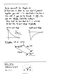
Use Malus’ Law to sketch below the fraction of the incident intensity I/I 0 that is transmitted as a<br />
function of β. Begin by tabulating coordinates (β,I/I 0 ) for a set of angles 0 ◦ ≤ β ≤ 90 ◦ , increasing β<br />
in 5 ◦ steps. Scale and label your graph appropriately, then plot your data table. Complete the graph by<br />
drawing a smooth curve through the plotted points. At what angle is ∆I/∆β the greatest? ............<br />
CONGRATULATIONS! YOU ARE NOW READY TO PROCEED WITH THE EXPERIMENT!<br />
Procedure and analysis<br />
The Faraday rotation apparatus consists of four basic components: the light source, the solenoid and power<br />
supply, the analyzer polariod and the optical detector.<br />
1: The light source<br />
The rectangular enclosure on the right side of the Faraday apparatus contains the light source, a red<br />
laser pointer of 650 nm wavelength. The laser light exits the enclosure through an integral polarizing<br />
filter so that the output of the light source is a 95% plane polarized wave. The laser beam can be<br />
adjusted to traverse the apparatus along its central axis and properly arrive at the optical detector<br />
by manipulating the four nylon thumb screws on the laser mount. Adjust the red spot at the input<br />
of the analyzer polaroid for a maximum meter reading.<br />
Note: The beam has been pre-aligned and should not require further adjustment. If there is no beam<br />
visible at the analyzer polaroid, see the lab instructor.
26 EXPERIMENT 3. FARADAY ROTATION<br />
2: The Solenoid<br />
The solenoid is a multilayer coil of wire 150 mm long that surrounds a sample of dielectric material,<br />
a SF59 glass rod of length l = 100 mm. When a current i flows throught the coil, a magnetic field<br />
develops around the coil. Inside the coil, this field vector ⃗ B points along the axis of the coil, in the<br />
direction of the analyzer polaroid, as shown in Figure 3.2. While the magnetic field does vary along<br />
the coil axis, this variation is not significant for samples shorter than and properly centered in the<br />
solenoid. The calibration constant for the solenoid is:<br />
B = 0.0111i (3.3)<br />
where i is in Amperes (A) and B in Tesla (T). To generate a magnetic field, set a voltage on the<br />
external power supply, then press the pushbutton on the Faraday apparatus to energize the solenoid<br />
briefly. The current flowing throught the solenoid is displayed on the power supply current meter.<br />
The coil resistance is R ≈ 2.6 Ω so that according to Ohm’s Law, V = iR, a setting of 2.6 V<br />
corresponds to a current of around 1 A. Avoid prolonged current flow through the solenoid; the coil<br />
will heat up and increase the temperature of the sample, altering your results.<br />
3: The analyzer polaroid<br />
This component is a polaroid film that can be rotated 360 ◦ in a calibrated mount graduated at 5 ◦<br />
intervals. A set screw is used to lock the protractor at a specific angle. Hold the protractor flat<br />
against the mount to prevent the angle, or meter reading, from changing as you gently tighten the<br />
set screw. Do not overtighten the assembly.<br />
4: The Detector<br />
The intensity of the transmitted beam is measured with a photodiode detector. The detector is<br />
sensitive to the visible as well as some of the infrared spectrum. The output of the detector is a<br />
current i d directly proportional to the input intensity I. The current flows through a resistor R,<br />
generating a voltage V = i d R that is displayed in units of 0.1 mV on the digital readout. A gain<br />
switch on the detector and gain adjustment knob on the front panel are used to set R and scale this<br />
output to the 0−1999 range of the four-digit 7-segment display, the region for which the detector<br />
output is linear. The displayed value represents the beam intensity in some arbitrary units, but since<br />
only relative intensity (I/I 0 ) measurements will be made, calibration of the beam intensity is not<br />
required.<br />
Part 1: Verification of Malus’ Law<br />
The task is to verify that Equation 3.1 is valid for this apparatus.<br />
• Turn on the power supply. Verify that the laser is turned off. The meter should display a zero<br />
reading, but may not. Why? Does the reading change with a gain adjustment? Test your hypothesis<br />
and note your observations below.<br />
.........................................................................<br />
• Switch on the power to the laser. The laser beam should be visible at the output of the light source;<br />
if it is not, see the lab instructor. The beam should also be visible at the input of the analyzer<br />
polaroid otherwise the apparatus needs to be aligned. Allow 5 minutes for the laser to warm up.
27<br />
• Slowly rotate the analyzer polaroid over 360 ◦ and note how the intensity readout varies. Adjust<br />
the detector gain to get a maximum reading that does not exceed the range of the display, 1999.<br />
This will yield the best display resolution for the measurement of I. This maximum reading is the<br />
unattenuated beam intensity I 0 . Record this value and corresponding angle below:<br />
I 0 = ...................., β 0 =....................<br />
• In 5 ◦ increments over a 180 ◦ range, record the beam intensity I. Set the angle carefully as described<br />
in the previous section; you may not need to tighten the set screw to take these measurements.<br />
β ( ◦ )<br />
I (mV)<br />
β ( ◦ )<br />
I (mV)<br />
β ( ◦ )<br />
I (mV)<br />
β ( ◦ )<br />
I (mV)<br />
Table 3.1: Intensity as a function of polarization angle<br />
• Use the PhysicaLab software to enter the data pairs (β,I) in the data window. Select scatter plot.<br />
Click Draw to plot a graph of your data. Select fit to: y= and enter A*(cos(B*x-C))**2+D in<br />
the fitting equation box. Note that the cosine function in the fitting equation expects an argument<br />
in radians while your data is in degrees. What is the conversion from degrees to radians? What is<br />
the physical meaning and unit of the four fit parameters A, B, C, D ?<br />
......................................................................<br />
......................................................................<br />
......................................................................<br />
From your graph, estimate and enter values for the fitting parameters A, B, C, D. Click Draw to<br />
perform a fit on your data. If the fit fails, you may need to reconsider some of your guesses. Label<br />
the axes and enter your name and a description of the data as part of the graph title. Click Print<br />
next to Draw to generate a hard copy of your graph. Record the fit results below:<br />
A = ..........±............... B = ..........±...............<br />
C = ..........±............... D = ..........±...............
28 EXPERIMENT 3. FARADAY ROTATION<br />
• Determine β 0 from the fit results and compare this value with a visual estimate of β 0 from the graph<br />
and the previously measured β 0 value. Evaluate your results in terms of measurement error.<br />
......................................................................<br />
......................................................................<br />
......................................................................<br />
The angle of interest is not actually β 0 , since I does not depend much on β near I 0 . The greatest change,<br />
hence the best resolution, in intensity I with β occurs when β = β m = β 0 ± 45 ◦ and I = I 0 /2. Does it<br />
matter which of the two angles is used? What difference do you note as β is increased?<br />
β m =......, ..........................................................<br />
Part 2: Determination of Verdet constant<br />
As shown in Equation 3.2, the change in polarization angle β is proportional to the magnetic field B and<br />
hence to the solenoid current i. To measure this rotation in the plane of polarization, set B = 0 and the<br />
analyzer angle to β m , the angle of the steepest slope, and record the intensity. Apply a current to the<br />
solenoid to generate a magnetic field B. The intensity reading will change. Rotate the analyzer polaroid<br />
until the intensity reading matches the previous B = 0 value, then estimate the new angle β.<br />
• Record below β for solenoid currents of i = 0,1,2,3 A. Be careful not to have the current turned on<br />
for any length of time because the coil windings will heat up and hence increase the temperature of<br />
the glass sample. The Verdet constant varies with temperature as well as with the frequency of light<br />
transmitted. Note your results below and include error estimates.<br />
I (A)<br />
β ( ◦ )<br />
Table 3.2: Rotation data, measured with protractor<br />
• Make a quick plot of the four points (i,β), then fit a straight line to your data by entering A+B*x<br />
in the fitting equation box. Use Equations 3.2 and 3.3 and the slope from your fit to estimate a<br />
value for the Verdet constant. Include an error calculation (refer to the Error rules in the Appendix,<br />
if necessary).<br />
ν = .............................. σ(ν) = ..............................<br />
.............................. ..............................<br />
.............................. ..............................<br />
ν = ...............±...............
29<br />
Part 3: Determination of Verdet constant, a better method<br />
You may have noticed that the rotation angle measured in the previous section is very small for the range<br />
of currents available. Along with the coarse 5 ◦ resolution of the analyzer scale, the resulting value for the<br />
Verdet constant exhibits a relatively large error, perhaps even large enough to make the result meaningless.<br />
However, you get a general feeling for the relationship between the solenoid current i and the resulting<br />
rotation β.<br />
You will now apply an indirect method that does not require angle measurements to determine the<br />
rotation angle and hence the Verdet constant. Using the Malus Equation 3.1 and solving for β yields:<br />
√<br />
I = I 0 cos 2 I<br />
β → β = arccos<br />
(3.4)<br />
I 0<br />
The rotation angle can thus be calculated, without the use of a protractor scale, by rotating the polarizer<br />
so that I = I 0 with B = 0, then applying some B, measuring the resulting I and evaluating Equation 3.4.<br />
This approach leads to a substantial improvement in resolution since both I and I 0 are measured<br />
precisely with the digital meter, however I does not change much near I 0 . As before, you want to maximize<br />
the resolution by taking measurements about the point I = I 0 /2, where ∆I/∆β is a maximum.<br />
• To set the analyzer polaroid to 45 ◦ relative to the incident beam:<br />
1. rotate the analyzer to get a maximum I 0 reading on the display;<br />
2. adjust the gain to maximize the display reading, allowing time for the display to settle;<br />
3. record the maximum intensity I 0 = ...............<br />
4. rotate the analyzer until I = I 0 /2, then secure it with the thumb screw.<br />
• The coil current is only readable during the time that the button is pressed and the coil has current<br />
flowing through the windings. This makes it difficult to set a specific current value, quickly, so that<br />
the coil does not heat up. However, because the coil is a resistor R that follows Ohm’s Law, V = iR,<br />
the coil current is directly proportional to the set voltage and you have a linear relationaship between<br />
i and V. You can thus calibrate the current i as a function of voltage V using two coordinate points.<br />
You determine one point by setting a voltage V max that causes a current i max just under 3 A to flow<br />
through the coil. The other calibration point is i = 0 wnen V = 0. The voltage V required to set<br />
any current i is given by the following relationship:<br />
( ) imax −0<br />
i = V. (3.5)<br />
V max −0<br />
• Fill Table 3.3 with a series of voltage values 0 < V ≤ V max . For each V entry in the table, adjust<br />
the power supply to set this output voltage. Press the button to energize the solenoid and note the<br />
solenoid current i and the resulting beam intensity I, then release the button and record the data in<br />
Table 3.3.<br />
• UseEquation3.3 tocalculate themagnetic fieldintensity B andEquation3.4tocalculate therotation<br />
angle β. Enter your data in Table 3.3<br />
• Plot your data as (B,β). The graph should approximate a straight line. Select fit to: y= and enter<br />
A*x+B in the fitting equation box and perform a linear fit on your data. Print a hard copy of your<br />
graph.<br />
A = ..........±.......... B = ..........±..........
30 EXPERIMENT 3. FARADAY ROTATION<br />
V (V)<br />
i (A)<br />
B (T)<br />
I<br />
β ( ◦ )<br />
Table 3.3: Rotation data calculated from intensity ratio<br />
From the slope, determine a value and error estimate for the Verdet constant.<br />
ν = .............................. σ(ν) = ..............................<br />
.............................. ..............................<br />
.............................. ..............................<br />
ν = ...............±...............<br />
IMPORTANT: BEFORE LEAVING THE LAB, HAVE A T.A. INITIAL YOUR WORKBOOK!<br />
Discussion<br />
Begin by tabulating and summarizing your Verdet constant results. Compare these in terms of error<br />
magnitudes. Do your results agree with the accepted value for the Verdet constant? Explain.<br />
The polarizer at the light source is not perfect. How would this affect your results?<br />
Why is an absolute calibration of the beam intensity not required?<br />
Is the presence of a non-zero value at the detector when the laser is turned off significant? How would<br />
you compensate for such a systematic error in your experiment?<br />
Summarize the results for Part 1. Is Malus’ Law a good model for the transmission properties of the<br />
polarizer?<br />
Comment on the results of Part 2. Is this a good way to determine the Verdet constant? Why? What<br />
change might be made to the apparatus to improve the results? Do your results provide a good estimate<br />
for the Verdet constant? How do you define a good estimate?<br />
Discuss your results of Part 3. How does this method of determining the Verdet constant improve upon<br />
the previous part? Explain.
first name (print) last name (print) student number TA initials grade<br />
Experiment 4<br />
Resistance<br />
When electrons, or other electric charge carriers (e.g. ions in a solution), are forced to move through a<br />
medium by an applied electric field (voltage, V), their motion is in most cases retarded by scattering off<br />
imperfections (impurities) and vibrating atoms in the medium. This resistance to the movement of charge<br />
is defined as<br />
R = V I<br />
where V is the voltage, or potential difference, applied<br />
across the material and I is the current, or rate of the<br />
movement of electric charge (electrons) in the material.<br />
The resistance R of a medium (resistor) is dependent on<br />
its chemical properties, geometry, temperature, external<br />
magnetic field, etc. The value of resistance may also<br />
show a dependence to the magnitude and polarity of the<br />
voltage V appliedacrossitsterminals, asisobservedwith<br />
a device made of semiconducting material.<br />
A resistor that is independent of the voltage applied<br />
across it is called an Ohmic resistor after George Simon<br />
Ohm (1787-1854) who described mathematically<br />
theelectrical characteristics of suchadevice. Ohm’sLaw<br />
states that the electric current I that flows in a conductor<br />
is proportional to the potential difference V between<br />
the ends of the conductor, and is inversely proportional<br />
to its resistance R.<br />
I = V R<br />
(4.1)<br />
Figure 4.1: IV relationship for resistor<br />
The unit for resistance is the ohm (Ω), and is derived<br />
from the units of voltage and current:<br />
1 ohm = 1 volt<br />
1 ampere .<br />
Figure 4.2: Basic resistor circuit<br />
Equation 4.1 is the equation of a straight line, with the slope equal to the resistance. By varying the<br />
voltage across a resistor and recording the current in each case, a IV graph can be plotted, and from that<br />
graph, the resistance of an unknown resistor can be established. A schematic representation of the simplest<br />
electric circuit is given in Figure 4.2.<br />
Ohmic resistors are used primarily to limit the current flow in an electric circuit. Several methods are<br />
used in their construction. For example, some resistors consist of a fine wire wound on an insulating core.<br />
The ones that you will use are formed from various carbon compounds.<br />
31
32 EXPERIMENT 4. RESISTANCE<br />
Kirchoff’s Laws<br />
ThebehaviourofanyelectriccircuitcanbeexaminedwiththeaidoftworulesdevelopedbyGustavKirchoff<br />
(1824-1887). These rules arise from the application of fundamental physical laws to electric circuits.<br />
A junction is a point in a circuit where a number of wires are connected together. Kirchoff’s current<br />
law, or junction rule, states that the total electron current entering a junction, or node, equals the total<br />
electron current leaving the junction, ∑ I = 0. Ineffect, it states that noelectrons are created or destroyed.<br />
This is the principle of conservation of electric charge.<br />
Kirchoff’s Voltage Law, or loop rule, states that the total work done on an electron by the voltage<br />
sources in a circuit equals the total work extracted from the electron while traversing the circuit. In<br />
following any such closed circuit loop, the gains in potential energy will be equal to the losses, so that<br />
∑ V = 0. This is the principle of conservation of energy.<br />
Effective resistance of resistors in series<br />
The effective resistance for R 1 and R 2 connected in<br />
series is R S . In general, the total resistance for any<br />
number N of resistors in series equals the sum of<br />
individual resistances, as shown by equation (4.2).<br />
N∑<br />
R S = R 1 +R 2 +···+R N = R i (4.2)<br />
i=1<br />
Applying Kirchoff’s Voltage Law (starting at O,<br />
traversing the loop clockwise) to the closed circuit<br />
loop in Figure 4.3 yields:<br />
V −IR 1 −IR 2 = 0<br />
V = IR 1 +IR 2<br />
V = I(R 1 +R 2 )<br />
V<br />
= R S = R 1 +R 2 .<br />
I<br />
Therefore, for two resistors connected in series,<br />
Figure 4.3: Resistors in series<br />
R S = R 1 +R 2 . (4.3)<br />
Effective resistance of resistors in parallel<br />
The effective resistance, R P , for any number N of<br />
resistors in parallel can be determined from equation<br />
(4.4).<br />
1<br />
R P<br />
= 1 R 1<br />
+ 1 R 2<br />
+···+ 1<br />
R N<br />
=<br />
N∑<br />
i=1<br />
1<br />
R i<br />
. (4.4)<br />
Figure 4.4: Resistors in parallel<br />
For two resistors connected in parallel:<br />
1<br />
R P<br />
= 1 R 1<br />
+ 1 R 2<br />
. (4.5)
33<br />
Review questions<br />
Show the relationship between the currents I, I 1 and I 2 at the junction O in Figure 4.4. This is an<br />
expression of Kirchoffs Current Law. If I = 7.5 A and I 1 = 4.5 A, what is the value of I 2 ?<br />
......................................................................<br />
Derive Equation 4.5 for the circuit shown in Figure 4.4. Begin by applying Kirchoff’s Current Law at<br />
junction O, and Kirchoff’s Voltage Law to the closed loops (1), and (2). Show a complete step by step<br />
solution.<br />
......................................................................<br />
......................................................................<br />
......................................................................<br />
CONGRATULATIONS! YOU ARE NOW READY TO PROCEED WITH THE EXPERIMENT!<br />
Procedure and analysis<br />
The experimental arrangement consists of a variable<br />
power supply to provide a voltage V to the<br />
test circuit. A potentiometer knob and voltmeter<br />
located on the front of the power supply are used<br />
to select a specific value of V. The voltmeter is<br />
connected in parallel to the voltage source.<br />
The output terminals of the power supply constitute<br />
an open circuit. The test circuit, or load, of<br />
effective resistance R is connected across the power<br />
supply to establish a closed circuit through which a<br />
current I can flow. This load may be one or more<br />
resistors in parallel or series, a diode, light bulb,<br />
motor or any other electrical component or system.<br />
To monitor the amount of current flowing in Figure 4.5: Experimental setup<br />
this closed circuit the power supply includes a current meter (ammeter) connected in series between the<br />
voltage source and the resistive load. Refer to Figure 4 for the circuit schematic. The digital meters have<br />
a measurement error of ± 0.5% plus one least significant digit (LSD) on the display.<br />
Part I: Single resistors<br />
In this exercise, you will determine R for a resistor from the slope of a line of best fit through a series of<br />
(I,V) data points. You will then compare the result with the nominal resistance of the component.<br />
• With the power supply off, check that the Range button is pressed. Rotate the voltage adjust knob<br />
on the power supply counterclockwise until it stops turning. The output voltage is now set to 0 V.
34 EXPERIMENT 4. RESISTANCE<br />
• Connect the circuit shown in Figure 4. Connect the resistor with the 1 Ω nominal resistance as the<br />
load resistor. We will call this resistor R 1 . The error, or tolerance, of the resistors is ± 5%.<br />
• Turn on the power supply. Press and hold the CC set button and use the curent adjust knob to<br />
set a maximum current to 2.0 A. This will limit the power supply current in case of a short circuit.<br />
• Use the voltage adjust knob to set the output voltage from 0.1 V to 1.0 V in increments of 0.1 V and<br />
at each step record in Table 4.1 the magnitude of the current flowing through the resistor. Remember<br />
to apply the proper units and significant figures to these results.<br />
V (V) 0.1 0.2 0.3 0.4 0.5 0.6 0.7 0.8 0.9 1.0<br />
σ(V) (V)<br />
I (A)<br />
σ(I) (A)<br />
Table 4.1: Experimental results for resistor R 1<br />
• Calculate σ(V) and σ(I), the errors in V and I, at V = 0.5 V and enter these results in Table 4.1.<br />
Include the other calculations as part of your Discussion.<br />
σ(V) = .............................. σ(I) = ..............................<br />
.............................. ..............................<br />
.............................. ..............................<br />
• Use the PhysicaLab software to enter the data pairs and their associated errors (I,V,σ(V),σ(I)) in<br />
the data window. Select scatter plot. Click Draw to generate a graph of your data. The graph<br />
should approximate a straight line. Select fit to: y= and enter A*x+B in the fitting equation<br />
box. Click Draw to perform a linear fit on your data. Label the axes and enter your name and a<br />
description of the data as part of the graph title. Click Print next to Draw to generate a hard<br />
copy of your graph. Do not use the browser print button to print your graph.<br />
• Enter below the experimental values for R 1 and σ(R) from the slope of the graph. Also tabulate the<br />
value and tolerance R 1 and σ(R) of resistor R 1 .<br />
(slope)R 1 = .................±.................Ω<br />
(nominal)R 1 = .................±.................Ω<br />
• Repeat theabove steps by connecting the circuit shown in Figure4usingtheresistor R 2 with nominal<br />
resistance of 0.75 Ω. as the load resistance. Enter your results in Table 4.2.
35<br />
V (V) 0.1 0.2 0.3 0.4 0.5 0.6 0.7 0.8 0.9 1.0<br />
σ(V) (V)<br />
I (A)<br />
σ(I) (A)<br />
Table 4.2: Experimental results for resistor R 1<br />
• Summarize below the values of R 2 from the slope of the graph and the the value displayed on the<br />
resistor R 2 .<br />
Part II: Resistors in series<br />
(slope)R 2 = .................±.................Ω<br />
(nominal)R 2 = .................±.................Ω<br />
• ReplacethesingleresistorusedinPartIbythetworesistorsconnectedinseriesasshowninFigure4.3.<br />
Set V=0.5 V and measure the corresponding value of I.<br />
V = ..........±.......... V<br />
I = ..........±.......... A<br />
Use Equation 4.1 to determine the experimental effective resistance R s . Apply the proper error<br />
propagation rule to evaluate the error σ(R s ) of the two resistors in series.<br />
R s = .............................. σ(R s ) = ..............................<br />
.............................. ..............................<br />
.............................. ..............................<br />
R s (Ohm ′ s Law) = ...............±...............Ω<br />
• Use the nominal component values for R 1 and R 2 and Equation 4.3 to calculate the theoretical<br />
effective resistance R s and error σ(R s ) of the two resistors in series:<br />
R s = .............................. σ(R s ) = ..............................<br />
.............................. ..............................<br />
.............................. ..............................<br />
R s (Series Law) = ...............±...............Ω
36 EXPERIMENT 4. RESISTANCE<br />
Part III: Resistors in parallel<br />
• Connect the two resistors in parallel. Set V = 0.5 V and measure the corresponding value of I.<br />
Calculate the experimental effective resistance R p and error σ(R p ) of the two resistors in parallel.<br />
R p = .............................. σ(R p ) = ..............................<br />
.............................. ..............................<br />
.............................. ..............................<br />
R p (Ohm ′ s Law) = ...............±...............Ω<br />
• Use the nominal component values and Equation 4.5 to calculate the theoretical resistance R p and<br />
the error σ(R p ) of the two resistors in parallel:<br />
R p = .............................. σ(R p ) = ..............................<br />
.............................. ..............................<br />
.............................. ..............................<br />
Part IV: IV characteristics of a diode<br />
R p (Parallel Law) = ...............±...............Ω<br />
As mentioned in the Introduction, many electrical devices do not<br />
obey Ohm’s law. A diode is a semiconducting device whose resistance<br />
not only depends on the voltage V applied across its terminals,<br />
but also on the polarity, or direction that the voltage is<br />
applied. The polarity of the diode is identified by a band at one<br />
end of the diode body. A diode is forward biased when the band<br />
end is connected to the negative (-) terminal of the power supply.<br />
It is reverse biased when the band end is connected to the positive<br />
(+) terminal of the power supply.<br />
• Set V = 0 V. Replace the resistors with the diode so that it<br />
is forward biased. Measure the current in the circuit over a<br />
range of voltages from 0.1 V to 1.0 V in steps of 0.1 V. Do<br />
not exceed 1 V as the diode may begin to conduct excessively,<br />
overheat and burn out. Present your results in Table 4.3.<br />
Figure 4.6: Current flow in a diode<br />
• Rearrange the diode so that it is connected in the reverse biased direction. Repeat the series of<br />
measurements and enter your data in Table 4.4.
37<br />
V (V) 0.1 0.2 0.3 0.4 0.5 0.6 0.7 0.8 0.9 1.0<br />
σ(V) (V)<br />
I (A)<br />
σ(I) (A)<br />
Table 4.3: Experimental results for forward biased diode<br />
V (V) -0.1 -0.2 -0.3 -0.4 -0.5 -0.6 -0.7 -0.8 -0.9 -1.0<br />
σ(V) (V)<br />
I (A)<br />
σ(I) (A)<br />
Table 4.4: Experimental results for reverse biased diode<br />
• On the graph paper below, plot your two data sets for the diode in a (V,I) format. Follow proper<br />
graphing techniques when plotting the points. Sketch a smooth line through your data points and<br />
properly label and title the graph. Describe quantitatively in your Discussion how the effective<br />
resistance of the diode varies with the applied voltage and polarity of the power supply.
38 EXPERIMENT 4. RESISTANCE<br />
V (V) 0.5 1.0 1.5 2.0 2.5 3.0 3.5 4.0 4.5 5.0<br />
I 1 (A)<br />
I 2 (A)<br />
I 3 (A)<br />
〈I〉 (A)<br />
Table 4.5: Experimental results for Tungsten filament<br />
Part V: Resistance characteristics of a heated filament<br />
In this exercise you are going to explore the temperature dependence of a resistor. The resistor in this case<br />
is the Tungsten filament of a low voltage light bulb. As the voltage applied across the filament is increased,<br />
the current causes the filament to increase in temperature and eventually begin to glow.<br />
• Replace the diode with the light bulb. Measure I and enter the results in Table 4.5. Estimate the<br />
voltage when the filament begins to glow. Repeat three times, then calculate 〈I〉 and 〈V〉. A different<br />
student should perform each set of readings.<br />
V on1 = ........V, V on2 = ........V, V on3 = ........V, 〈V on 〉 = ........V<br />
• On the grid below, plot the (V,〈I〉) results for the tungsten filament. Sketch a smooth line through<br />
the set of data and properly label and title your graph. On the line, identify the voltage 〈V on 〉.
39<br />
IMPORTANT: BEFORE LEAVING THE LAB, HAVE A T.A. INITIAL YOUR WORKBOOK!<br />
Discussion<br />
Summarize your results in a table, presenting the data properly rounded off according to the magnitude<br />
of the associated errors and labelled with the appropriate physical units.<br />
Compare your experimental resistance values with the manufacturers given values. Do the two sets<br />
of values agree within their margin of error? Explain. Why is there such a large difference between the<br />
magnitude of your experimental error for a component and the component’s tolerance value? Why do you<br />
think that the manufacturer specifies such a large value for the tolerance of the component?<br />
Review your results for the silicon diode.<br />
Describeindetailthebehaviourofaforwardbiaseddiodeasthevoltage acrosstheterminalsisincreased<br />
from 0 V to 1 V. Identify with voltage values the pertinent features.<br />
A real diode can only dissipate a limited amount of heat. Referring to your graph of the diode IV<br />
curve, what would you expect to observe as the voltage across a forward biased diode continues to be<br />
increased above 1 V? What additional component(s) would need to be added to a diode circuit to prevent<br />
excessive current from flowing through the diode?<br />
Describe the behaviour of a reverse biased diode as V is increased from 0 V to 1 V. What assumptions<br />
can you make regarding the operation of a reverse biased diode as the voltage is increased beyond 1 V?<br />
Explain. Do you think that there is a value of V beyond which this assumption is no longer valid?<br />
Review your results for the tungsten filament.<br />
Does the (V,I) curve that you graphed represent the resistance R of the filament as a function of<br />
voltage, or does it represent the reciprocal of the resistance 1/R (conductance)?<br />
Does the graph of the tungsten filament give any clues as to the behaviour of a resistor with temperature?<br />
Does the resistance change significantly as the filament gets brighter? Does it increase or decrease?<br />
Is there any outstanding feature in the graph near the voltage V at which you firstnoticed that the filament<br />
begins to glow?<br />
................................................................................<br />
................................................................................<br />
................................................................................<br />
................................................................................<br />
................................................................................<br />
................................................................................<br />
................................................................................<br />
................................................................................
40 EXPERIMENT 4. RESISTANCE<br />
Identifying a resistor value and tolerance<br />
The value of a resistor is typically identified on the component as a numeric value or by a series of colored<br />
bands. The orientation of the bands can be determined by selecting the First Band as the band closest to<br />
the end of the resistor body. The color of this band makes up the first digit of the resistance value.<br />
Figure 4.7: Resistor colour bands<br />
Colour<br />
First Band Second Band Third Band Fourth Band<br />
First Digit Second Digit Multiplier Tolerance<br />
Black 0 0 10 0 –<br />
Brown 1 1 10 1 –<br />
Red 2 2 10 2 –<br />
Orange 3 3 10 3 –<br />
Yellow 4 4 10 4 –<br />
Green 5 5 10 5 –<br />
Blue 6 6 10 6 –<br />
Violet 7 7 10 7 –<br />
Gray 8 8 10 8 –<br />
White 9 9 10 9 –<br />
Gold – – 10 −1 ± 5% of R<br />
Silver – – 10 −2 ± 10% of R<br />
No Colour – – – ± 20% of R<br />
For example, the resistance R of a resistor whose bands are yellow, violet, red, gold is<br />
R = yellow-violet×red±gold<br />
R = 47×10 2 Ω±(5% of 47×10 2 Ω)<br />
R = 4700±200 Ω (error rounded to one significant figure) = (4.7±0.2)×10 3 Ω
first name (print) last name (print) student number TA initials grade<br />
Experiment 5<br />
Electron charge-to-mass ratio<br />
This experiment was designed to determine the charge-to-mass ratio, e/m, for an electron. Commonly<br />
called the Bainbridge Experiment in honour of the scientist who developed the method, this experiment<br />
exhibits an ingenious combination of electromagnetic theory and mechanics.<br />
Figure 5.1: The Bainbridge Tube<br />
As seen in Figure 5.1, the central component of the apparatus is a large vacuum tube (Bainbridge<br />
tube). Inside the tube, a vertical metal cylinder with a narrow slot cut in its side, the anode, encloses an<br />
axially mounted wire, the cathode.<br />
The cathode heater power supply provides a voltage across the cathode wire and causes a significant<br />
electron current flow through the wire. Collisions between these energetic electrons and the atoms in the<br />
wire ejects some electrons from the material, forming an electron cloud around the cathode.<br />
The anode power supply is then used to set the anode at a potential V more positive than that of<br />
the cathode, to create a radial electric field inside the cylinder that will accelerate the negatively charged<br />
41
42 EXPERIMENT 5. ELECTRON CHARGE-TO-MASS RATIO<br />
electrons toward the outer anode. Some of these electrons shoot through the slot in the anode. After<br />
escaping, they will continue to move in a straight line with a constant speed v since there is no electric<br />
field outside the anode.<br />
Work-energy theorem demands that the work done by the electric field in accelerating an electron is<br />
equal to the change in the electron’s potential energy,<br />
∆(K.E.) = W = eV. (5.1)<br />
Assumingthat theinitial kineticenergy oftheelectrons nearthesurfaceof thecathodeiszero, Equation 5.1<br />
yields the value for the kinetic energy an electron has after it escapes through the slot in the anode.<br />
Changing the anode voltage V controls this kinetic energy and, therefore, the speed v of the electron,<br />
K.E. = 1 2 mv2 ⇒ v =<br />
√<br />
2V<br />
( e<br />
m)<br />
. (5.2)<br />
The second stage of this experiment involves magnetic forces. Two large Helmholtz coils, positioned<br />
above and below the Bainbridge tube, are used to create a uniform magnetic field in the tube. With this<br />
arrangement, the direction of the magnetic field intensity ( B) ⃗ is vertical, perpendicular to the velocity ⃗v<br />
of the electrons. The magnetic force ( F) ⃗ experienced by an electron is given by the vector cross-product<br />
⃗F = e⃗v × B ⃗ and F = ∣F<br />
⃗ ∣ = evB. (5.3)<br />
Since ⃗ F is always perpendicular to ⃗v, it does no work on the electron, and cannot change its kinetic energy<br />
or its speed. The magnetic force acts as a centripetal force, F c = ma c , making the electrons move in a<br />
circle of radius r. The plane of the circle is perpendicular to ⃗ B. From mechanics, the centripetal force is<br />
F = evB = F c = ma c = mv2<br />
r . (5.4)<br />
Rearranging Equation 5.4 so that only e/m remains on the left-hand side yields<br />
e<br />
m = 2V<br />
r 2 B2. (5.5)<br />
Thus the charge-to-mass ratio for an electron, e/m, can be determined from V, r and B.<br />
The anode potential V can be measured accurately using a voltmeter, or read directly from the power<br />
supply. The magnetic field strength, B, depends of the size of the Helmholtz coils and the current, I,<br />
flowing in them. For the coils you will use in this experiment, B is given by<br />
B =<br />
(<br />
1.96×10 −4 T/A<br />
)<br />
×I , (5.6)<br />
where B is in units of Tesla (T) and I in units of Ampere (A).<br />
The radius of the circular orbit, r, is determined from the dimensions of the experimental apparatus<br />
itself in the following manner. The tube is filled with mercury vapour. Electrons colliding with mercury<br />
atoms induce these atoms to emit a faint purple light, making the electron path visible in a dark room.<br />
Fivemetalpostsaremountedinthetubeatknowndistancesfromthecathode. Byvaryingthemagnetic<br />
field strength B at constant anode voltage V, or by varying V at constant B, the electron beam is moved<br />
until it strikes a post. At that moment we match precisely the size of the circular path the electrons take,<br />
to one of the known cathode-to-pole distances of the tube itself (see Table 5.2 in the experimental section).<br />
Note that we match the diameter d (d = 2r) of the circular path, and not its radius, r.<br />
This is essentially the strategy we will pursue for this experiment: use the measured voltage V and a<br />
known size of the circular orbit r, determine the magnetic field strength B from the measured current I,<br />
and substitute these values into Equation (5.5) to calculate the ratio e/m.
43<br />
The electron beam emerging from the slot spreads out slightly as it goes around the tube. There are<br />
two main reasons for this spreading. First, not all the electrons leave the slot with exactly the speed v<br />
given by Equation (5.2), nor are all of the velocities ⃗v exactly perpendicular to ⃗ B. Also, collisions with the<br />
mercury may change the velocity of the electrons and therefore, the radius of their orbit. To reduce the<br />
experimental imperfections due to this spreading, we will position the beam so that it is split “in half” by<br />
the post when determining e/m.<br />
Review questions<br />
• Derive an equation for the speed of the electrons v in terms of the measurable variables V, B, and<br />
r. This is accomplished by solving Equations (5.2) and (5.5) for v instead of e/m. Show a complete<br />
step by step solution. Start with the work-energy theorem:<br />
W = eV = 1 2 mv2<br />
......................................................................<br />
......................................................................<br />
......................................................................<br />
• Derive an expression for the error σ(e/m) in the equation below. You will need the equation in Part<br />
III of this lab. Begin by applying a change of variables as shown in the Appendix to develop a clear<br />
step by step solution.<br />
e/m = 2∗slope∗B −2<br />
......................................................................<br />
......................................................................<br />
......................................................................<br />
• Report an accepted value for the likely strength of the Earth’s magnetic field B E in St. Catharines<br />
and the electron charge-to-mass ratio, e/m. You may use a <strong>Physics</strong> textbook, a reference book, or<br />
even the internet to find this value. Cite your source in detail.<br />
B E = ......................... , from ................................<br />
e/m = ......................... , from ................................<br />
CONGRATULATIONS! YOU ARE NOW READY TO PROCEED WITH THE EXPERIMENT!
44 EXPERIMENT 5. ELECTRON CHARGE-TO-MASS RATIO<br />
Procedure and Analysis<br />
Figure 5.2: Schematic Diagram of Electrical Apparatus<br />
Part I: Measurement of the Earth’s magnetic field<br />
Asktheinstructortoexplaintheoperationofanyoftheelectrical componentswhichyoudonotunderstand.<br />
• Switch on the anode power supply A and set the anode voltage to V = 25V. The helipot dial for the<br />
anode power supply has been scaled to read voltage directly, at 10V/turn, with an accuracy of ±1%.<br />
• Switch on the cathode heater power supply C and slowly increase the current until the electron beam<br />
is visible. DO NOT exceed 5A cathode heater current or you will burn out the filament. Consult<br />
the instructor if the tube does not operate properly.<br />
• Observe the electron beam which, due to the Earth’s magnetic field B E , should be slightly curved.<br />
• Switch on the magnetic field power supply B and slowly increase the coil current, until the electron<br />
beam looks straight. Now the magnetic field B generated by the coil is of equal magnitude<br />
and opposite direction to the Earth’s magnetic field B E , making the net magnetic field around the<br />
Bainbridge tube equal to zero. At this point, the electrons should experience no net magnetic force,<br />
F = evB = 0, and their path should remain straight for all values of the accelerating voltage V.<br />
• Vary the anode voltage through the 15–35 V range and adjust the coil current to produce the least<br />
amount of sideways beam movement. Ideally, there should be no movement, however the setup is<br />
not perfect. Record this estimated zero field current in Table 5.1 and repeat the procedure n = 5<br />
times, setting I n initially to zero each time. Calculate I 0 , the average of the I n values. The error in<br />
all current measurements is 0.3% +0.01 A. Is this error representative of the error in I 0 ? Explain.<br />
How should the error in I 0 be calculated?<br />
..............................................................................<br />
..............................................................................
45<br />
n 1 2 3 4 5 I 0 = Σ I n /n<br />
I n (A)<br />
Table 5.1: Determination of I 0 from average of five measured I n values<br />
Note: In order to obtain the value of coil current I affecting the electron beam, the zero field I 0<br />
must always be subtracted from the meter reading, i.e. I = I m −I 0 .<br />
• Use the value of I 0 to calculate the magnitude of the magnetic field of the Earth B E at the Bainbridge<br />
apparatus.<br />
Part II: Constant anode voltage<br />
B E = ..................±..................T<br />
Post No. d (m) r (m) V (V) I 0 (A) I m (A) I (A) B (T) e m (C/kg) v (m/s)<br />
1 0.065<br />
2 0.078<br />
3 0.090<br />
4 0.103<br />
5 0.115<br />
Table 5.2: Calculation of e/m and electron velocity v<br />
In this section you will determine the average e/m and the standard deviation σ(e/m) of a series of<br />
e/m values calculated from experimental data.<br />
• Set the anode voltage on power supply A to 25 V. Increase the coil current to increase the curvature<br />
of the electron beam until it is split by the outermost post (Post No. 5). Make sure that the beam<br />
is not being reflected from the inner surface of the Bainbridge tube.<br />
• Record I m and V in the appropriate row of Table 5.2. Calculate B, r, e/m and the speed v of the<br />
electrons as decribed in the theory section of this lab. Enter the results in Table 5.2.<br />
( )<br />
B = 1.96×10 −4 T/A ×I = ..................<br />
r = 1 ×d = ..................<br />
2<br />
e<br />
m = 2V<br />
r 2 B 2 = .................. = ..................<br />
v = 2V = .................. = ..................<br />
rB<br />
• Repeat these measurements and calculations for each of the remaining posts, keeping V constant.<br />
Include these calculations as part of your Discussion.
46 EXPERIMENT 5. ELECTRON CHARGE-TO-MASS RATIO<br />
i e m<br />
e m − 〈 e m<br />
〉 ( em − 〈 e m<br />
〉) 2<br />
i v v −〈v〉 (v −〈v〉) 2<br />
1 1<br />
2 2<br />
3 3<br />
4 4<br />
5 5<br />
〈 em 〉 = variance = 〈v〉 = variance =<br />
σ ( e m<br />
) = σ(v) =<br />
Table 5.3: Calculation of standarddeviation of e/m and v. Here, variance(x) = σ 2 (x) ≈ 1 N<br />
∑ Ni=1<br />
(x i −〈x〉) 2 .<br />
Since the error in r, σ(r) is not known, σ(e/m) cannot be determined via the usual error propagation rules.<br />
Instead, a statistical calculation of the standard deviation of e/m, σ(e/m), provides the best possible<br />
estimate of error.<br />
• Use Table 5.3 as your worksheet to calculate the average and the standard deviation of e/m and v.<br />
The value of σ(x) provides the desired error estimate for 〈x〉. Thus you may now complete this part of the<br />
experiment by reporting the final results for e/m and v. You may need to adjust the number of significant<br />
figures you report here, to be consistent with your calculated error estimate (it does not make sense to<br />
report 1.2345±0.1, for example).<br />
e/m = ..................±.................. C/kg<br />
Part III: Constant coil current<br />
v = ..................±.................. m/s<br />
In this section you will determine e/m and σ(e/m) by performing a linear least squares fit on a set of<br />
graphed data points. Equation (5.5) can be rewritten to indicate that V varies with r 2 .<br />
V = B2<br />
2<br />
( e<br />
m)<br />
r 2 =<br />
( )<br />
B 2 e<br />
r 2 (5.7)<br />
2m<br />
and is the equation of a straight line through the origin, with B 2 e/(2m) as the slope. To test this relation,<br />
I and hence B will be fixed and V varied to position the beam at the various posts.<br />
• Set the anode voltage V to the minimum required to produce a stable beam. Record this value.<br />
• Position thebeamat theinnermost post(No.1) by varyingthecoil currentI m andhencethemagnetic<br />
field strength B. Record the value of I m necessary to do this.<br />
• Leaving I m fixed, measure the value of V required to position the beam at the various posts. Record<br />
these values in Table 5.4.<br />
• Fill in Table 5.4. The measurement error in the voltage V is σ(V) = ±0.02 V.
47<br />
Post No. r (m) r 2 (m 2 ) V (V) σ(V) (V) I 0 (A) I m (A) I (A)<br />
1<br />
2<br />
3<br />
4<br />
5<br />
Table 5.4: Data for determining e/m and σ(e/m) using a linear least squares fit<br />
• Using the Physicalab software, enter the coordinate pairs (r 2 ,V) into the data window. Also enter<br />
the error values for these two quantities. Since we do not know the magnitude of the error in the<br />
radius r, set σ(r) = σ(r 2 ) = 0. Be sure to enter the data in the appropriate columns. Select scatter<br />
plot. Click Draw to generate a graph of your data. Your data should approximate a straight line<br />
and the error bars should be displayed. If this is not the case, check your data and then redraw<br />
the graph. Select fit to: y= and enter A+B*x in the fitting equation box. Here B is the fitting<br />
parameter corresponding to the slope of the straight line, not the magnetic field vector B. Label<br />
the axes and enter your name as part of the graph title. Click Draw then Print to generate a<br />
printout of your graph. Every student should print their own graph.<br />
• Record below the value of the slope and standard deviation of the slope:<br />
slope = B2 e<br />
2m = ..................±.................. V/m2 (5.8)<br />
• From your graph results, calculate the voltage that would be required to place the beam at a post<br />
d = 0.130 m from the cylinder cathode. Show a complete solution, no error estimate required.<br />
..............................................................................<br />
..............................................................................<br />
..............................................................................<br />
..............................................................................<br />
..............................................................................<br />
In the following calculations be sure to not round off your values prematurely. Do not perform further<br />
calculations with a result after it has been truncated according to the position of the significant digit of<br />
the associated error.<br />
• Calculate B and σ(B) from I and σ(I). The error in the measurement of the current is 0.3 % of the<br />
I value plus one least significant digit (LSD) of the meter display. Since the meter scale was set to
48 EXPERIMENT 5. ELECTRON CHARGE-TO-MASS RATIO<br />
display current in units of Amperes (A), with three digits of resolution (0.00), the LSD corresponds<br />
to 0.01 A and hence the total error in the current is σ(I) = (0.003 I +0.01) A.<br />
I = ..................±.................. A<br />
B = .............................. σ(B) = ..............................<br />
.............................. ..............................<br />
.............................. ..............................<br />
B = ..................±.................. T<br />
• With Equation 5.8 expressed in terms of e/m, calculate e/m and σ(e/m) using the values of slope<br />
and B:<br />
e/m = 2∗slope∗B −2 σ(e/m) = ..............................<br />
.............................. ..............................<br />
.............................. ..............................<br />
e/m = ..................±.................. C/Kg<br />
IMPORTANT: BEFORE LEAVING THE LAB, HAVE A T.A. INITIAL YOUR WORKBOOK!<br />
Discussion<br />
Tabulate your final results for e/m and the magnitude of the earth’s magnetic field B E . There is no need<br />
to duplicate any of the data tables contained in the lab workbook, or to make an extensive review of the<br />
lab theory and procedures. Attach your computer printouts and worksheets to this Discussion. Here are<br />
a few ideas on the issues you need to address in your Discussion; as always, this is not a complete list.<br />
Do your two results for the electron charge to mass ratio e/m agree with one another? Explain how the<br />
errors magnitudes associated with these values are used to assert or deny this agreement. How do these<br />
values compare with the accepted value of e/m from your review section?<br />
Does your values for the Earth’s magnetic field strength B E obtained from Part I agree with the<br />
accepted value from the review section of this experiment?<br />
InPart II,whereVwas kept constant, doyour results for theelectron velocity v agree withthe expected<br />
electron velocity for V = 25 V?<br />
Do we need an error estimate for the voltage V? Explain.<br />
What are the most significant sources of experimental error and how could these errors be minimized?
first name (print) last name (print) student number TA initials grade<br />
Experiment 6<br />
Diffraction of light by a grating<br />
The optical diffraction grating is a glass or plastic plate with many fine, parallel grooves spaced the same<br />
distance d from each other on its surface. When monochromatic light from a distant source or laser hits the<br />
grating, each groove re-radiates the light as spherical waves in phase with the incident wave. The diffracted<br />
light beams are formed by the superposition of many spherical waves. In the case where the incident light<br />
beam is a parallel beam, and is incident at right angles to the grating, the diffraction pattern will be generated<br />
by groups of beams parallel at a given angle α to the direction of the incident beam. as in Figure 6.1.<br />
Since the beam incident onto the grating is in<br />
phase, a given diffracted beam will be offset from<br />
its parallel neighbour by a distance dsinα. When<br />
this distance is equal to an integer number m of<br />
wavelengths λ of the incident light, the two beams<br />
are in phase and will exhibit constructive interference<br />
by displaying a series of bright regions on the<br />
screen. These interference maxima are given by:<br />
dsinα = mλ, m = 0,±1,±2,... (6.1)<br />
where λ is the wavelength, d is the grating spacing,<br />
and m is an integer called the order number. If<br />
the path difference between adjacent beams is (m+<br />
1/2)λ, then destructive interference will result in<br />
dark regions, or interference minima, on the screen. Figure 6.1: Diffraction by a grating<br />
The zero-order beam m = 0 is a continuation of the<br />
incidentbeam(i.e. α = 0). Therearetwofirstorder<br />
beams, m = ±1 at angles given by sinα = ±λ/d, two second order beams m = ±2 at sinα = ±2λ/d, et<br />
cetera. Hence the measurement of the angle α, together with the order number m, gives the ratio λ/d,<br />
and if either λ or d is known, the other can be calculated.<br />
Note that if λ > d one doesn’t get diffraction maxima of order m ≥ 1. On the other hand, if λ is much<br />
less than d the low order maxima might not be resolved as the corresponding angles become much too<br />
small. Thus, the diffraction effect becomes important when λ is not too small a fraction of d. To diffract<br />
X-rays, electrons, or neutron matter waves, one needs a diffraction grating whose d is comparable with the<br />
wavelength of the waves. It turns out that crystal materials have interatomic spacings comparable with<br />
the λ of X-rays. X-ray diffraction is now a standard way of determining the atomic arrangements in a<br />
crystal.<br />
49
50 EXPERIMENT 6. DIFFRACTION OF LIGHT BY A GRATING<br />
To experimentally determine a value for the grating distance d of a diffraction grating a monochromatic<br />
light source of a known wavelength λ is used as the incident beam. The beam is diffracted from the grating<br />
and generates an interference pattern on a screen a distance D from the grating. On the screen the distance<br />
L between pairs of bright spots from the diffraction of order ±m can be measured and Equation 6.1 can<br />
be used to calculate the grating distance d. Note that this equation assumes that the beams from adjacent<br />
grating slits are parallel, that is, that D ≫ L.<br />
A Hydrogen atom consists of a positively<br />
charged proton making up the atomic nucleus and<br />
a negatively charged electron orbiting this nucleus.<br />
Quantum Theory predicts that the electron may<br />
only find itself in one of n = 1,2,3,... discrete orbits,<br />
or energy levels, around the nucleus.<br />
When a Hydrogen atom is subjected to an electric<br />
discharge, its one electron may absorb some of<br />
this energy. Whenthis happens, theelectron makes<br />
a transition from an orbit n 1 to an orbit n 2 where<br />
n 2 > n 1 . The electron eventually decays back to a<br />
lowerorbit, releasingthissurplusenergyintheform<br />
of a photon of one of several specific wavelengths λ.<br />
Some of these transitions radiate photons that have<br />
the wavelength of visible light andcan thus bemeasured<br />
with a spectrometer.<br />
Figure 6.2: Electronic energy transitions of H 2<br />
Johann J. Balmer (1825-1898) discovered that for the Hydrogen atom the series of energy transitions<br />
wavelengths from an initial energy level n > 2 to the energy level n = 2, the Balmer series, are approximately<br />
given by:<br />
λ =<br />
[<br />
R( 1<br />
2 2 − 1 n 2 )] −1<br />
, (6.2)<br />
The value of the Rydberg constant R in the Balmer equation is determined by fitting this empirical<br />
equation to experimental data and is equal to R = 1.097×10 7 m −1 .<br />
The electron energy level transitions that produce<br />
wavelengths in the visible region are from an<br />
initial orbit n = 3,4 or 5 to a final orbit n = 2,<br />
as shown in Figure 6.2. These transitions will be<br />
visible as red (n = 3 → 2), blue (n = 4 → 2), and<br />
purple(n = 5 → 2) lines inthespectrumof molecular<br />
Hydrogen (H 2 ) from an H 2 discharge tube. The<br />
unscattered combination of these three colors will<br />
have a pink colour.<br />
The spectrometer is an optical instrument that<br />
usesaprismoradiffractiongratingtoscatter anincident<br />
light beam of interest into component wavelengths.<br />
The grating used in this spectrometer is<br />
chosen to optimally view the first order (m = ±1)<br />
diffraction pattern of the incident beam.<br />
When the light from the H 2 discharge lamp is<br />
viewed through a spectrometer, the three colors<br />
linesscatter at different angles symmetrically about Figure 6.3: Diffraction of the H 2 spectrum<br />
thedirectpathoftheincidentlight, asinFigure6.3.
51<br />
Review questions<br />
• Derive an equation for the diffraction grating distance d as a function of the given variables m and<br />
λ, and the measured variables L and D. Begin with Equation 6.1 and the relationship tanα = L/2D<br />
from Figure 6.4. Use the approximation that tanα ≈ sinα if D ≫ L. Show a complete step by step<br />
solution.<br />
......................................................................<br />
......................................................................<br />
......................................................................<br />
......................................................................<br />
• Derive an equation for σ(λ), the error in λ. This error equation will be needed in Part II of this lab.<br />
Begin by rearranging Equation 6.1 in terms of λ. Express the equation as a product of terms, then<br />
perform a change of variables to develop a complete step by step solution, as shown in the Appendix.<br />
λ = d m sin(α) = d∗m−1 ∗sin(α) = A∗B ∗C<br />
......................................................................<br />
......................................................................<br />
......................................................................<br />
......................................................................<br />
......................................................................<br />
......................................................................<br />
• Argue using Equation 6.1 that there can be no diffraction pattern if λ > d.<br />
......................................................................<br />
......................................................................<br />
CONGRATULATIONS! YOU ARE NOW READY TO PROCEED WITH THE EXPERIMENT!
52 EXPERIMENT 6. DIFFRACTION OF LIGHT BY A GRATING<br />
Procedure and analysis<br />
Part I: Determining the spacing of a diffraction grating<br />
In this part of the experiment you will determine<br />
the spacing d of a glass grating by passing a laser<br />
beam through it and examining the diffraction pattern<br />
projected on a screen. The laser beam is parallel<br />
and monochromatic, with wavelength<br />
λ±σλ = 632.8±0.5 nm.<br />
• Check that the screen and grating surface are<br />
perpendicularto the incident beam, and measure<br />
the distance D between the grating and<br />
the screen, as shown in Figure 6.4.<br />
D = ...........±...........m<br />
Figure 6.4: Experimental setup for Part I.<br />
• Mount a sheet of graph paper on the screen and carefully mark the series of interference maxima.<br />
Identify the straight path m = 0 maximum. Each student must make and analyse their own<br />
interference pattern. Measure the distance L between the centres of pairs of spots of order m, (+m<br />
to −m) for m = ±1 to m = ±10. Record your results in Table 6.1.<br />
• With L and D measured, use the equation you derived in the review exercise to calculate d for the<br />
ten measurements of L. With sinα ≈ tanα, d = 2mλD/L. Use Table 6.1 to calculate the average<br />
value 〈d〉 and standard deviation σ(d) of d.<br />
m L (m) d (m) (d−〈d〉) (m) (d−〈d〉) 2 (m)<br />
±1<br />
±2<br />
±3<br />
±4<br />
±5<br />
±6<br />
±7<br />
±8<br />
±9<br />
±10<br />
〈d〉 = variance =<br />
σ(d) =<br />
Table 6.1: Calculation of 〈d〉 and σ(d). Here, variance(x) = σ 2 (x) ≈ 1 N<br />
∑ Ni=1<br />
(x i −〈x〉) 2 .
53<br />
Part II: Determining the wavelengths of the Balmer spectrum of H 2<br />
The light source is a hydrogen discharge tube. This<br />
source illuminates aslit at one end of the collimator<br />
tube, and a lens at the other end makes a parallel<br />
beam of the light passing through the slit. The<br />
beam is diffracted by the grating and collected by<br />
the front lens of the telescope, which focuses the<br />
light on a set of cross-hairs. The telescope can rotate<br />
around the grating, its angular position with<br />
respect to an arbitrary zero given by an angular<br />
scale on the base of the instrument. Proceed as follows,<br />
remembering never to touch the grating as it<br />
is easily damaged and is expensive to replace.<br />
• Rotate the telescope to a position opposite the collimator. Looking through the telescope you should<br />
see a sharp image of the slit, its colour the same as that of the light emanating from the discharge<br />
tube. Gently lock the telescope in place with the knob located at the centre of the telescope base.<br />
• Turn the fine-adjust knob located on the right side of the telescope base to centre the diagonally<br />
oriented cross hairs on an edge of the slit image. A screw on the collimator near the light source<br />
allows adjustment of the slit width. Be sure to have the slit and crosshairs in focus.<br />
• Read the position of the telescope from the angular scale on the base. This can be done to a precision<br />
of 1 ′ ( ± one minute, 60 ′ = 1 ◦ ) . To read the scale:<br />
1. Locate the “0” line on the vernier scale, and note which main scale division it is immediately<br />
after, e.g. 212 ◦ 30 ′ on the main scale in Figure 6.5. Note that the numbers on the main and<br />
vernier scales increase from right to left, and not from left to right as you are used to reading.<br />
2. Scan along the line where the main and vernier scales meet, and note which one vernier scale<br />
division is directly in line with a main scale division, e.g. 17 ′ on the vernier scale in Figure 6.5.<br />
3. Add the main and vernier scale readings to obtain the angular scale reading, e.g. 212 ◦ 30 ′ +17 ′ =<br />
212 ◦ 47 ′ in Figure 6.5. Enter your measurement in Table 6.2.<br />
Figure 6.5: Example of Angular Vernier Scale Reading – 212 ◦ 47 ′
54 EXPERIMENT 6. DIFFRACTION OF LIGHT BY A GRATING<br />
• Unlock the telescope and slowly rotate it to the right until the first violet slit image is in the field of<br />
view. Lock the telescope, and use the fine-adjust knob until the cross hairs are again situated on the<br />
same edge of the slit image as was used before. Read the position indicated on the angular scale and<br />
let its value be θ +1 . This value corresponds to the direction of the diffracted beam with m = +1 for<br />
the violet spectral line.<br />
• Unlock the telescope, rotate it to the left of center until the firstviolet image is seen again. Determine<br />
its angular position θ −1 , corresponding to the diffracted beam with m = −1. Repeat the above<br />
measurements for the blue and purple spectral lines and enter your data in the first row of Table 6.2.<br />
• Convert your data values from degrees and minutes to decimal degrees, recalling that 1 ◦ = 60 ′ , and<br />
enter these in the second row of Table 6.2.<br />
◦ , ′<br />
◦<br />
Pink (θ 0 ) Violet (θ +1 ) Violet (θ −1 ) Blue (θ +1 ) Blue (θ −1 ) Red (θ +1 ) Red (θ −1 )<br />
Table 6.2: Measurements for the spectral lines of H 2 in degrees/minutes and decimal degrees<br />
The diffraction angle α ±1 for a particular colour is the measured angle of deviation θ ±1 of that colour<br />
from the light’s direct path reference angle θ 0 . Calculating the difference between the angular positions of<br />
the pink and coloured lines will give you α ±1 , i.e.<br />
α ±1 = |θ 0 −θ ±1 | (6.3)<br />
• Calculate from the data in Table 6.2 the values of the diffraction angle α ±1 for the three lines of the<br />
H 2 spectrum. There will be two results for each colour, α ±1 , one for each side of the reference angle<br />
θ 0 . Calculate the average 〈α〉 of these two angles then estimate the error with σ(α) = 1 2 |α +1 −α −1 |.<br />
line α +1 α −1 〈α〉 σ(α)<br />
Violet (α V )<br />
Blue (α B )<br />
Red (α R )<br />
Table 6.3: Calculated diffraction angles for the spectral lines of H 2<br />
The diffraction grating used in the spectrometer is made with a line density of<br />
N ±σ(N) = 600±1 lines/mm.<br />
This is not the same value as the grating spacing in Part I. The line density and grating spacing are related<br />
via d = 1/N. The distance d between the lines and error σ(d) for the grating used in this spectrometer is<br />
d = .......... mm,<br />
σ(d) = .................= .................= .......... mm
55<br />
• Calculate a wavelength λ(α) and the error σ(λ(α)) of the violet spectral line of H 2 . Show the<br />
calculations below. Record this data in Table 6.4.<br />
λ V = d m sin(α V) σ(λ V ) =<br />
...................... .............................................<br />
...................... .............................................<br />
...................... .............................................<br />
λ V = ...............±...............m<br />
• Calculate a wavelength λ(α) and the error σ(λ(α)) of the blue spectral line of H 2 . Show the calculations<br />
below. Record this data in Table 6.4.<br />
λ B = d m sin(α B) σ(λ B ) =<br />
...................... .............................................<br />
...................... .............................................<br />
...................... .............................................<br />
λ B = ...............±...............m<br />
• Calculateawavelength λ(α)andtheerrorσ(λ(α)) oftheredspectrallineofH 2 . Showthecalculations<br />
below. Record this data in Table 6.4.<br />
λ R = d m sin(α R) σ(λ R ) =<br />
...................... .............................................<br />
...................... .............................................<br />
...................... .............................................<br />
λ R = ...............±...............m
56 EXPERIMENT 6. DIFFRACTION OF LIGHT BY A GRATING<br />
• Use the Balmer Equation 6.2 to calculate the theoretical wavelengths λ(Balmer) of the violet, blue<br />
and red lines of the H 2 spectrum. Show below the calculation for the wavelength of the violet spectral<br />
line produced by the n = 5 → n = 2 energy transition of the Hydrogen atom. Record this data and<br />
your results for the other two colours in Table 6.4. Include all your other calculations as part of the<br />
Discussion.<br />
......................................................................<br />
......................................................................<br />
......................................................................<br />
line transition λ(α) σ(λ(α)) λ(Balmer)<br />
Violet<br />
Blue<br />
Red<br />
Table 6.4: Calculated λ(α) from angles 〈α〉 and λ(Balmer) from Equation 6.2<br />
IMPORTANT: BEFORE LEAVING THE LAB, HAVE A T.A. INITIAL YOUR WORKBOOK!<br />
Discussion<br />
Summarize your results for Part I. Tabulate your calculated value for the spacing of the diffraction grating<br />
and the associated error. Consider the experimental arrangement and the theory on which this value<br />
depends and comment on ways that this error might be reduced.<br />
Compare the magnitude of the value of the grating spacing and the wavelength of the laser light used<br />
to produce the interference pattern. Is the ratio of these two values as you would expect? Explain.<br />
Summarize your results for Part II. Compare the values of the wavelengths obtained experimentally<br />
for the first order diffraction of the Hydrogen spectrum with those theoretically predicted by the Balmer<br />
equation. Do the two sets of results agree within the margin of your experimental error? Explain.<br />
Consider the experimental arrangement used in this part of the experiment. Outline some of the<br />
difficulties encountered while measuring the spectral lines of Hydrogen and suggest some possible solutions.<br />
Did these difficulties contribute a significant error to the experimental results? How might this error be<br />
minimized?<br />
The resolution of the protractor scale on the spectrometer is one minute or 0.0167 ◦ , yet we estimated<br />
the error σ(α) in Table 6.3 as σ(α) = 1 2 |α +1−α −1 |. Why was the resolution value not used? Is the equation<br />
for σ(α) a valid method of calculating the error in α? Explain.
first name (print) last name (print) student number TA initials grade<br />
Appendix A<br />
Review of math basics<br />
Fractions<br />
a<br />
c + b d = ad+bc<br />
cd<br />
; If<br />
a<br />
c = b d<br />
, then ad = cb and<br />
ad<br />
bc = 1.<br />
Quadratic equations<br />
Squaring a binomial: (a+b) 2 = a 2 +2ab+b 2<br />
Difference of squares: a 2 −b 2 = (a+b)(a−b)<br />
The two roots of a quadratic equation ax 2 +bx+c = 0 are given by x = −b±√ b 2 −4ac<br />
.<br />
2a<br />
Exponentiation<br />
(a x )(a y ) = a (x+y) ,<br />
a x<br />
a y = ax−y , a 1/x = x√ a , a −x = 1 a x , (ax ) y = a (xy)<br />
Logarithms<br />
Given that a x = N, then the logarithm to the base a of a number N is given by log a N = x.<br />
For the decimal number system where the base of 10 applies, log 10 N ≡ logN and<br />
Addition and subtraction of logarithms<br />
log1 = 0 (10 0 = 1)<br />
log10 = 1 (10 1 = 10)<br />
log1000 = 3 (10 3 = 1000)<br />
Given a and b where a,b > 0: The log of the product of two numbers is equal to the sum of the individual<br />
logarithms, and the log of the quotient of two numbers is equal to the difference between the individual<br />
logarithms .<br />
log(ab) = loga+logb<br />
( a<br />
log = loga−logb<br />
b)<br />
The following relation holds true for all logarithms:<br />
loga n = nloga<br />
57
58 APPENDIX A. REVIEW OF MATH BASICS<br />
Natural logarithms<br />
It is not necessary to use a whole number for the logarithmic base. A system based on “e” is often used.<br />
Logarithms using this base log e are written as “ln”, pronounced “lawn”, and are referred to as natural<br />
logarithms. This particular base is used because many natural processes are readily expressed as functions<br />
of natural logarithms, i.e. as powers of e. The number e is the sum of the infinite series (with 0! ≡ 1):<br />
Trigonometry<br />
e =<br />
∞∑<br />
n=0<br />
1<br />
n! = 1 0! + 1 1! + 1 2! + 1 +··· = 2.71828...<br />
3!<br />
Pythagoras’ Theorem states that for a right-angled triangle c 2 = a 2 + b 2 .<br />
Defining a trigonometric identity as the ratio of two sides of the triangle,<br />
there will be six possible combinations:<br />
sinθ = b c<br />
cscθ = c b<br />
cosθ = a c<br />
secθ = c a<br />
tanθ = b a = sinθ<br />
cosθ<br />
cotθ = a b = cosθ<br />
sinθ<br />
sin(θ ±φ) = sinθ cosφ±cosθsinφ sin2θ = 2sinθ cosθ 180 ◦ = π radians = 3.15159...<br />
cos(θ ±φ) = cosθ cosφ∓sinθsinφ cos2θ = 1−2sin 2 θ 1 radian = 57.296... ◦<br />
tan(θ ±φ) = tanθ±tanφ<br />
1∓tanθ tanφ<br />
tan2θ = 2tanθ<br />
1−tan 2 θ<br />
sin 2 θ+cos 2 θ = 1<br />
To determine what angle a ratio of sides represents, calculate the inverse of the trig identity:<br />
if sinθ = b ( ) b<br />
c , then θ = arcsin c<br />
For any triangle with angles A,B,C respectively opposite the sides a,b,c:<br />
The sine waveform<br />
a<br />
sinA = b<br />
sinB = c<br />
sinC<br />
If we increase θ at a constant rate from<br />
0 to 2π radians and plot the magnitude<br />
of the line segment b = c sinθ as a function<br />
of θ, a sine wave of amplitude c and<br />
period of 2π radians is generated.<br />
Relative to some arbitrary coordinate<br />
system, the origin of this sine wave<br />
is located at a offset distance y 0 from the<br />
horizontal axis and at a phase angle of θ 0<br />
from the vertical axis. Thesine wave referenced<br />
from this (θ,y) coordinate system<br />
is given by the equation<br />
y = y 0 +csin(θ +θ 0 )<br />
, (sine law) c2<br />
= a 2 +b 2 −2ac cosC. (cosine law)
first name (print) last name (print) student number TA initials grade<br />
Appendix B<br />
Error propagation rules<br />
• The Absolute Error of a quantity Z is given by σ(Z), always ≥ 0.<br />
• The Relative Error of a quantity Z is given by σ(Z)<br />
|Z|<br />
, always ≥ 0.<br />
• To determine the error in a quantity Z that is the sum of other quantities, you add the absolute errors<br />
of those quantities (Rules 2,3 below). To determine the error in a quantity Z that is the product of<br />
other quantities, you add the relative errors of those quantities (Rules 4,5 below).<br />
Relation<br />
Error<br />
1. Z = cA σ(Z) = |c|σ(A) (Use only if A is a single term, i.e. Z = 3x.)<br />
2. Z = A+B +C +··· σ(Z) = σ(A)+σ(B)+σ(C)+···<br />
3. Z = A−B −C −··· σ(Z) = σ(A)+σ(B)+σ(C)+··· (Error terms are always added.)<br />
4. Z = A×B ×C ×···<br />
σ(Z)<br />
|Z|<br />
= σ(A)<br />
|A|<br />
+ σ(B)<br />
|B|<br />
+ σ(C)<br />
|C|<br />
+···<br />
5. Z = A σ(Z)<br />
B<br />
|Z|<br />
= σ(A)<br />
|A|<br />
+ σ(B)<br />
|B|<br />
6. Z = A b σ(Z)<br />
|Z|<br />
= |b| σ(A)<br />
|A|<br />
(Note the absolute value of the power.)<br />
7. Z = sinA σ(Z) = σ(sinA) = |sin[A+σ(A)]−sin[A−σ(A)]|<br />
2<br />
(Similar for cosA)<br />
8. Z = logA σ(Z) = σ(logA) = |log[A+σ(A)]−log[A−σ(A)]|<br />
2<br />
• a,b,c,...,z represent constants<br />
• A,B,C,...,Z represent measured or calculated quantities<br />
• σ(A),σ(B),σ(C),...,σ(Z) represent the errors in A,B,C,...,Z, respectively.<br />
How to derive an error equation<br />
Let’s use the change of variable method to determine the error equation for the following expression:<br />
• Begin by rewriting Equation B.1 as a product of terms:<br />
y = M √<br />
0.5 kx(1−sinθ) (B.1)<br />
m<br />
59
60 APPENDIX B. ERROR PROPAGATION RULES<br />
y = M ∗ m −1 ∗ [ 0.5 ∗ k ∗ x ∗ (1−sinθ)] 1/2<br />
(B.2)<br />
= M ∗ m −1 ∗ 0.5 1/2 ∗ k 1/2 ∗ x 1/2 ∗ (1−sinθ) 1/2 (B.3)<br />
• Assign to each term in Equation B.3 a new variable name A,B,C,... , then express v in terms of<br />
these new variables,<br />
y = A ∗ B ∗ C ∗ D ∗ E ∗ F<br />
(B.4)<br />
• With σ(y) representing the error or uncertainty in the magnitude of y, the error expression for y is<br />
easily obtained by applying Rule 4 to the product of terms Equation B.4:<br />
σ(y)<br />
|y|<br />
= σ(A)<br />
|A|<br />
+ σ(B)<br />
|B|<br />
+ σ(C)<br />
|C|<br />
+ σ(D)<br />
|D|<br />
+ σ(E)<br />
|E|<br />
+ σ(F)<br />
|F|<br />
(B.5)<br />
• Select from the table of error rules an appropriate error expression for each of these new variables as<br />
shown below. Note that F requires further simplification since there are two terms under the square<br />
root, so we equate these to a variable G:<br />
A = M, σ(A) = σ(M) Rule 1<br />
σ(B)<br />
B = m −1 ,<br />
|B|<br />
= |−1| σ(m)<br />
|m|<br />
= σ(m)<br />
|m|<br />
Rule 6<br />
C = 0.5 1/2 σ(C)<br />
,<br />
|C|<br />
= ∣ 1 σ(0.5)<br />
2∣<br />
|0.5|<br />
= 0 since σ(0.5) = 0<br />
D = k 1/2 σ(D)<br />
,<br />
|D|<br />
= ∣ 1 σ(k)<br />
2∣<br />
|k|<br />
= σ(k)<br />
2|k|<br />
Rule 6<br />
E = x 1/2 σ(E)<br />
,<br />
|E|<br />
=<br />
1 σ(x)<br />
2<br />
|x|<br />
= σ(x)<br />
2|x|<br />
Rule 6<br />
F = G 1/2 σ(F)<br />
,<br />
|F|<br />
= ∣ 1 σ(G)<br />
2∣<br />
|G|<br />
= σ(G)<br />
2|G|<br />
Rule 6<br />
G = 1−sinθ, σ(G) = σ(1)+σ(sinθ) = 0+ | sin[θ+σ(θ)]−sin[θ−σ(θ)] |<br />
2<br />
Rules 3,6<br />
• Finally, replace the error terms into the original error Equation B.5, simplify and solve for σ(y) by<br />
multiplying both sides of the equation with y:<br />
[ σ(M)<br />
σ(y) = |y| + σ(m) + σ(k)<br />
|M| |m| 2|k| + σ(x) | sin[θ +σ(θ)]−sin[θ −σ(θ)] |<br />
+<br />
2|x| |4(1−sinθ)|<br />
]<br />
(B.6)
first name (print) last name (print) student number TA initials grade<br />
Appendix C<br />
Graphing techniques<br />
A mathematical function y = f(x) describes the one to one<br />
relationship between the value of an independent variable x<br />
andadependentvariabley. Duringanexperiment, weanalyse<br />
some relationship between two quantities by performing a seriesof<br />
measurements. Toperformameasurement, weset some<br />
quantity x to a chosen value and measure the corresponding<br />
value of the quantity y. A measurement is thus represented<br />
by a coordinate pair of values (x,y) that defines a point on a<br />
two dimensional grid.<br />
Thetechniqueofgraphingprovidesaveryeffective method<br />
of visually displaying the relationship between two variables.<br />
By convention, the independent variable x is plotted along the<br />
horizontal axis(x-axis) andthedependentvariabley isplotted<br />
along the vertical axis (y-axis) of the graph. The graph axes<br />
should be scaled so that the coordinate points (x,y) are well<br />
distributed across the graph, taking advantage of the maximum<br />
display area available. This point is especially important<br />
when results are to be extracted directly form the data<br />
presented in the graph. The graph axes do not have to start<br />
at zero.<br />
Scale each axis with numbers that represent the range of<br />
values being plotted. Label each axis with the name and unit<br />
of the variable being plotted. Include a title above the graphing<br />
area that clearly describes the contents of the graph being<br />
plotted. Refer to Figure C.1 and Figure C.2.<br />
Figure C.1: Proper scaling of axes<br />
The line of best fit<br />
Figure C.2: Improper scaling of axes<br />
Supposethere is a linear relationship between x and y, so that<br />
y = f(x) is the equation of a straight line y = mx+b where m is the slope of the line and b is the value<br />
of y at x = 0. Having plotted the set of coordinate points (x,y) on the graph, we can now extract a value<br />
for m and b from the data presented in the graph.<br />
Draw a line of ’best fit’ through the data points. This line should approximate as well as possible the<br />
trend in your data. If there is a data point that does not fit in with the trend in the rest of the data, you<br />
should ignore it.<br />
61
62 APPENDIX C. GRAPHING TECHNIQUES<br />
The slope of a straight line<br />
The slope m of a straight-line graph is determined by<br />
choosing two points, P 1 = (x 1 ,y 1 ) and P 2 = (x 2 ,y 2 ),<br />
on the line of best fit, not from the original data, and<br />
evaluating Equation C.1. Note that these two points<br />
should be as far apart as possible.<br />
m = rise<br />
run<br />
m = ∆y<br />
∆x = y 2 −y 1<br />
x 2 −x 1<br />
(C.1)<br />
Error bars<br />
Figure C.3: Slope of a line<br />
All experimental values are uncertain to somedegree due<br />
to the limited precision in the scales of the instruments<br />
used to set the value of x and to measure the resulting<br />
value of y. This uncertainty σ of a measurement is<br />
generally determined from the physical characteristics of<br />
themeasuringinstrument, i.e. thegraduations of ascale.<br />
When plotting a point (x,y) on a graph, these uncertainties<br />
σ(x) and σ(y) in the values of x and y are indicated<br />
using error bars.<br />
For any experimental point (x±σ(x),y ±σ(y)), the<br />
Figure C.4: Error Bars for Point (x,y)<br />
error bars will consist of a pair of line segments of length<br />
2σ(x) and 2σ(y), parallel to the x and y axes respectively<br />
and centered on the point (x,y). The true value lies within the rectangle formed by using the error<br />
bars as sides. The rectangle is indicated by the dotted lines in Figure C.3. Note that only the error bars,<br />
and not the rectangle are drawn on the graph.<br />
The uncertainty in the slope<br />
Figure C shows a set of data points for a linear relationship.<br />
The slope is that of line 2, the line of best fit<br />
through these points. The uncertainty in this slope is<br />
taken to be one half the difference between the line of<br />
maximum slope line 1 and the line of miinimum slope,<br />
line 3:<br />
σ(slope) = slope max −slope min<br />
2<br />
(C.2)<br />
The lines of maximum and minimum slope should go<br />
through the diagonally opposed vertices of the rectangles<br />
defined by the error bars of the two endpoints of the<br />
graph, as in Figure C.<br />
Figure C.5: Determining slope error
63<br />
Logarithmic graphs<br />
In science courses you will encounter a great number of functions and relationships, both linear and nonlinear.<br />
Linearfunctionsaredistinguishedbyaproportionalchangeinthevalueofthefunctionwithachange<br />
in value of one of the variables, and can be analyzed by plotting a graph of y versus x to obtain the slope m<br />
andvertical intercept b. Non-linear functionsdonot exhibitthis behaviour, butcan beanalyzed inasimilar<br />
manner with some modification. For example, a commonly occuring function is the exponential function,<br />
y = ae bx ,<br />
(C.3)<br />
where e = 2.71828..., and a and b are constants.<br />
Plotted on linear (i.e. regular) graph paper, the<br />
function y = ae bx appears as in Figure C.6. Taking<br />
the natural logarithm of both sides of equation<br />
(C.3) gives<br />
lny = ln<br />
(ae bx)<br />
lny = lna+ln<br />
(e bx)<br />
lny = lna+bxlne<br />
lny = lna+bx (since lne = 1)<br />
Equation (C.4) is the equation of a straight line<br />
for a graph of lny versus x, with lna the vertical Figure C.6: The exponential function y = ae bx .<br />
intercept, and b the slope. Plotting a graph of lny<br />
versus x (semilogarithmic, i.e. logarithmic on the vertical axis only) should result in a straight line, which<br />
can be analyzed.<br />
There are two ways to plot semilogarithmic data for analysis:<br />
1. Calculate the natural logarithms of all the y values, and plot lny versus x on linear scales. The slope<br />
and vertical intercept can then be determined after plotting the line of best fit.<br />
2. Use semilogarithmic graph paper. On this type of paper, the divisions on the horizontal axis are<br />
proportional to the number plotted (linear), and the divisions on the vertical axis are proportional to<br />
the logarithm of the number plotted (logarithmic). This method is preferable since only the natural<br />
logarithms of the vertical coordinates used to determine the slope of the lines best fit, minimum and<br />
maximum slope need to be calculated.<br />
Semilogarithmic graph paper<br />
The horizontal axis is linear and the vertical axis is logarithmic. The vertical axis is divided into a series<br />
of bands called decades or cycles.<br />
• Each decade spans one order of magnitude, and is labelled with numbers 1, 2, 3, 4, 5, 6, 7, 8, 9, 1.<br />
• the second “1” represents 10× what the first “1” does, the third 10× the second, et cetera, and<br />
• there is no zero on the logarithmic axis since the logarithm of zero does not exist.<br />
A logarithmic axis often has more than one decade, each representing higher powers of 10. In Figure C.7,<br />
the axis has 3 decades representing three consecutive orders of magnitude. For instance, if the data to be<br />
plotted covered the range 1 → 1000, the lowest decade would represent 1 → 10 (divisions 1, 2, 3, ..., 9),
64 APPENDIX C. GRAPHING TECHNIQUES<br />
Figure C.7: A 3-Decade Logarithmic Scale.<br />
the second decade 10 → 100 (divisions 10, 20, 30, ..., 90) and the third decade 100 → 1000 (divisions 100,<br />
200, 300, ...900, 1000).<br />
Another advantage of using a logarithmic scale is that it allows large ranges of data to be plotted. For<br />
instance, plotting 1 → 1000 on a linear scale would result in the data in the lower range (e.g. 1 → 100)<br />
being compressed into a very small space, possibly to the point of being unreadable. On a logarithmic<br />
scale this does not occur.<br />
Calculating the slope on semilogarithmic paper<br />
The slope of a semilogarithmic graph is calculated in the usual manner:<br />
m = slope<br />
= rise<br />
run<br />
∆(vertical)<br />
=<br />
∆(horizontal) .<br />
For ∆(vertical) it is necessary to calculate the change in the logarithm of the coordinates, not the change<br />
in the coordinates themselves. Using points (x 1 ,y 1 ) and (x 2 ,y 2 ) from a line on a semilogarithmic graph of<br />
y versus x and Equation C.4, the slope of the line is obtained.<br />
m = rise<br />
run<br />
m = lny 2 −lny 1<br />
x 2 −x 1<br />
m = ln(y 2/y 1 )<br />
x 2 −x 1<br />
(C.4)<br />
Note that the units for m will be (units of x) −1 since lny results in a pure number.<br />
Analytical determination of slope<br />
There are analytical methods of determining the slope m and intercept b of a straight line. The advantage<br />
of using an analytical method is that the analysis of the same data by anyone using the same analytical<br />
method will always yield the same results. Linear Regression determines the equation of a line of best fit<br />
by minimizing the total distance between the data points and the line of best fit.<br />
To perform“Linear Regression” (LR), onecan usethe preprogrammedfunction of a scientific calculator<br />
or program a simple routine using a spreadsheet program. Based on the x and y coordinates given to it, a<br />
LR routine will return the slope m and vertical intercept b of the line of best fit as well as the uncertainties<br />
σ(m) and σ(b) in these values. Be aware that performing a LR analysis on non-linear data will produce<br />
meaningless results. You should first plot the data points and determine visually if a LR analysis is indeed<br />
valid.