Diploma thesis

3 Complex square well potential
away but we can see again that even for τ = 0.2 only this k-state remains while the n-state has
already nearly vanished.
3.4 Related Systems
The last section of this chapter is dedicated to some related systems. On the one hand we
consider the asymmetric potential where area 1 and 3 do not yield the same extension and which
thus represents a generalization of our so far regarded system. From this we will get an impression
in what extent the particular symmetry influences our system and w will be able to evaluate an
appropriate interpretation of (3.34). On the other hand we compare the results of our model with
these two quite similar real valued systems in order to underline new properties the potential well
exhibits only in the complex case.
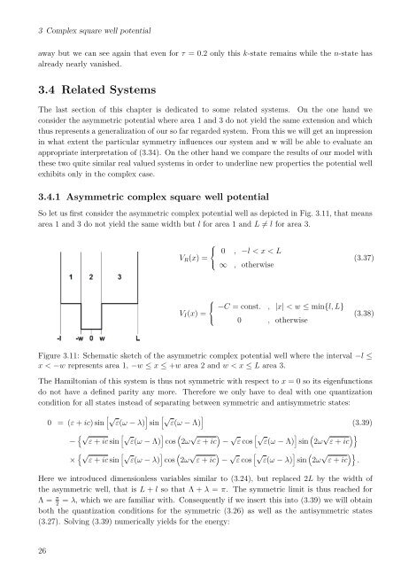
3.4.1 Asymmetric complex square well potential
So let us first consider the asymmetric complex potential well as depicted in Fig. 3.11, that means
area 1 and 3 do not yield the same width but l for area 1 and L ≠ l for area 3.
⎧
⎨ 0 , −l < x < L
V R (x) =
⎩ ∞ , otherwise
(3.37)
⎧
⎨ −C = const. , |x| < w ≤ min{l, L}
V I (x) =
⎩ 0 , otherwise
(3.38)
Figure 3.11: Schematic sketch of the asymmetric complex potential well where the interval −l ≤
x < −w represents area 1, −w ≤ x ≤ +w area 2 and w < x ≤ L area 3.
The Hamiltonian of this system is thus not symmetric with respect to x = 0 so its eigenfunctions
do not have a defined parity any more. Therefore we only have to deal with one quantization
condition for all states instead of separating between symmetric and antisymmetric states:
0 = (ε + ic) sin [ √ ε(ω − λ)
]
sin
[√ ε(ω − Λ)
]
− { √
ε + ic sin
[√ ε(ω − Λ)
]
cos
(
2ω
√
ε + ic
)
−
√ ε cos
[√ ε(ω − Λ)
]
sin
(
2ω
√
ε + ic
)}
× { √
ε + ic sin
[√ ε(ω − λ)
]
cos
(
2ω
√
ε + ic
)
−
√ ε cos
[√ ε(ω − λ)
]
sin
(
2ω
√
ε + ic
)}
.
(3.39)
Here we introduced dimensionless variables similar to (3.24), but replaced 2L by the width of
the asymmetric well, that is L + l so that Λ + λ = π. The symmetric limit is thus reached for
Λ = π = λ, which we are familiar with. Consequently if we insert this into (3.39) we will obtain
2
both the quantization conditions for the symmetric (3.26) as well as the antisymmetric states
(3.27). Solving (3.39) numerically yields for the energy:
26