Detailed analysis of MSE spectra

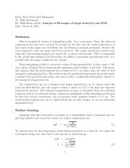
From: Steve Scott
To: Howard Yuh, Bob Granetz
Re: MSE Memo #8: Detailed Analysis of MSE FFT Spectra
Date: July 2, 2003
Motivation
Previous memos in this series have carried out standard Müeller Matrix analysis for the mse
diagnostic optics including the effect of imperfect mirrors which introduce a phase shift δ and
a non-unity reflectivity ratio r m for the S- versus P- polarizations. The calculated photon
intensity at the photomultiplier tubes is:
[
4I net = (I b + I 0 ) 1 + r m + r ]
m − 1
√ (cos(A) + sin(A) sin(B))
2
[
+I 0 cos(2γ) r m − 1 + r ]
m + 1
√ (cos(A) + sin(A) sin(B))
2
+I 0 sin(2γ) √ 2r m [cos(δ) cos(B) + sin(δ)(sin(A) − sin(B) cos(A))] (1)
where the time-dependent retardances imposed by the two pem’s are A(t) = R 1 cos(ω 1 t)
and B(t) = R 2 cos(ω 2 t). Customarily, we operate both pem’s with a retardance amplitude
R 1 = R 2 = π.
I wrote a small idl procedure to calculate I net (t) directly from Eq. 1 given user-supplied
values for the mirror properties, the pem retardances, the pitch-angle of the magnetic field in
the coordinate frame of the mse diagnostic. Then I performed standard fft decomposition
to determine the expected fft amplitudes for various assumptions about the diagnostic
performance. This provides a check on analytic calculations of the fft amplitudes, which
are obtained using the expansions:
cos(R cos(ωt)) =
∞∑
J 0 (R) + (−1) n J 2n (R) cos(2nωt)
n=1
sin(R cos(ωt)) =
∞∑
2 (−1) n−1 J 2n−1 (R) cos((2n − 1)ωt). (2)
n=1
Note that the terms sin(A(t)) sin(B(t)) and sin(B(t)) cos(A(t)) in Eq. 1 will give rise to a
large number of fft components at frequencies corresponding to sums and differences of ω 1
and ω 2 .
It’s convenient to group the terms into two sets: ‘ideal’ frequencies at which we expect
nonzero fft amplitudes for mirrors having no phase shift (δ = 0), and additional ‘nonideal’
terms that arise when the mirrors introduce a phase shift. These frequencies are listed in
Table 1. Since ω 1 ≈ ω 2 , the ideal frequencies tend to be grouped around the even multiplies
of the pem frequencies, while the nonideal frequencies tend to be groupe around the odd
multiples. As we will see in subsequent plots, the expected fft spectrum is quite rich, with
significant fft amplitudes out to at least 4 times the fundamental pem frequency, and with
4-5 split components near each harmonic.
1

Ideal Nonideal
0 ω 1
2ω 1 3ω 1
4ω 1 5ω 1
6ω 1 7ω 1
8ω 1 9ω 1
2ω 2 ω 2
4ω 2 3ω 2
6ω 2 5ω 2
8ω 2 7ω 2
ω 1 ± ω 2 9ω 2
3ω 1 ± ω 2 2ω 1 ± ω 2
5ω 1 ± ω 2 4ω 1 ± ω 2
7ω 1 ± ω 2 6ω 1 ± ω 2
3ω 2 ± ω 1 8ω 1 ± ω 2
5ω 2 ± ω 1 3ω 2 ± 2ω 1
7ω 2 ± ω 1 4ω 1 ± 3ω 2
3ω 1 ± 3ω 2 5ω 2 ± 2ω 1
5ω 1 ± 3ω 2 6ω 1 ± 3ω 2
5ω 2 ± 3ω 1 5ω 2 ± 4ω 1
5ω 1 ± 5ω 2 7ω 2 ± 2ω 1
7ω 1 ± 3ω 2
7ω 2 ± 3ω 1
9ω 1 ± 1ω 2
9ω 2 ± 1ω 1
Table 1: Frequencies at which we expect nonzero fft amplitudes for ideal and nonideal
mirrors. Nonideal mirrors will have the frequency components listed in both columns.
Expected Signals When only One PEM is Operating
If we turn off pem#2, then
I net = M p · M P EM1 · M m · S v . (3)
Doing the matrix multiplication with Maple yields an intensity
4I net = (I 0 + I b )(1 + r m + r m − 1
√ cos(A) 2
+I 0 cos(2γ)(r m − 1 + r m + 1
√ cos(A)) 2
+I 0 sin(2γ) √ 2r m (cos(δ) + sin(δ) sin(A)). (4)
Making the usual substitutions yields the intensities:
I ω1 = I 0 sin(δ) √ r m J 1 (A 1 )
√
2
sin(2γ)
2

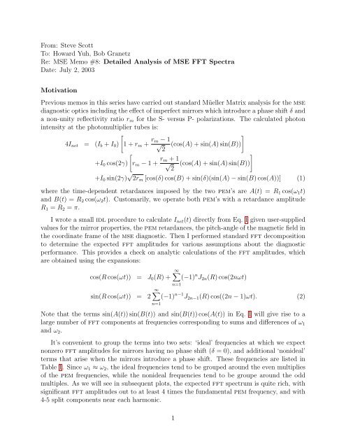
Figure 1: Computed fft spectrum for mse operating with both pems at their customary
retardance (R 1 = R 2 = π) for imperfect mirrors having a large phase shift, δ = 30 o . A
field-line pitch angle of 24 o with respect to the pem optics is assumed. The light green
lines represent frequencies that are expected from ideal mirrors. The yellow lines reprsent
frequencies that are expected from the non-ideal mirror behavior. The important point of
this figure is that non-negligible fft amplitudes occur only at those frequencies where we
expect them - all of the fft features correspond to either a known ideal or a known non-ideal
frequency.
3

Figure 2: Computed fft spectrum for mse operating with both pems at their customary
retardance (R 1 = R 2 = π) for perfect mirrors having no shift, δ = 0 o and equal reflectivity
for S- and P- polarization. A field-line pitch angle of 24 o with respect to the pem
optics is assumed. Magenta vertical lines indicate the frequencies corresponding to simple
harmonics of the pem frequencies. The blue lines represent the fft amplitudes that are
close to frequencies expected for ideal mirrors listed in Table 1. In subsequent plots, green
lines represent fft amplitudes that are near frequencies expected from the non-ideal mirror
characteristics.
4

Figure 3: fft spectrum for mse operating with both pems at their customary retardance
(R 1 = R 2 = π) for perfect mirrors having no shift, δ = 0 o and equal reflectivity for S- and
P- polarization. A field-line pitch angle of 24 o with respect to the pem optics is assumed.
This is the same case as the previous plot, Fig. 2, but plotted on a log scale to allow the
identification of low-amplitude components.
5

Figure 4: fft spectrum for mse operating with both pems at their customary retardance
(R 1 = R 2 = π) for imperfect perfect mirrors having a moderate phase shift, δ = 5 o and
unity reflectivity for S- and P- polarization. A field-line pitch angle of 24 o with respect to
the pem optics is assumed. Note that the mirror’s phase shift creates new but rather small
fft amplitudes near the first and third harmonics of both pem frequencies.
6

Figure 5: fft spectrum for mse operating with both pems at their customary retardance
(R 1 = R 2 = π) for imperfect perfect mirrors having a moderate phase shift, δ = 5 o and
unity reflectivity for S- and P- polarization. A field-line pitch angle of 24 o with respect to
the pem optics is assumed. Note that the mirror’s phase shift creates new but rather small
fft amplitudes near the first and third harmonics of both pem frequencies. This is the same
case as the previous plot, Fig. 4, but plotted on a log scale to allow the identification of
low-amplitude components.
7

Figure 6: fft spectrum for mse operating with both pems at their customary retardance
(R 1 = R 2 = π) for imperfect perfect mirrors having a large phase shift, δ = 30 o and unity
reflectivity for S- and P- polarization. A field-line pitch angle of 24 o with respect to the
pem optics is assumed. Note that the mirror’s phase shift creates new but rather small fft
amplitudes near the first and third harmonics of both pem frequencies.
8

Figure 7: fft spectrum for mse operating with both pems at their customary retardance
(R 1 = R 2 = π) for imperfect perfect mirrors having a large phase shift, δ = 30 o and unity
reflectivity for S- and P- polarization. A field-line pitch angle of 24 o with respect to the
pem optics is assumed. Note that the mirror’s phase shift creates new but rather small fft
amplitudes near the first and third harmonics of both pem frequencies. This is the same
case as the previous plot, Fig. 6, but plotted on a log scale to allow the identification of
low-amplitude components.
9

Figure 8: fft spectrum for mse operating with both pems at their customary retardance
(R 1 = R 2 = π) for imperfect perfect mirrors having a very large phase shift, δ = 60 o and
unity reflectivity for S- and P- polarization. A field-line pitch angle of 24 o with respect to
the pem optics is assumed. Note that the mirror’s phase shift creates new but rather small
fft amplitudes near the first and third harmonics of both pem frequencies.
10

Figure 9: fft spectrum for mse operating with both pems at their customary retardance
(R 1 = R 2 = π) for imperfect perfect mirrors having a very large phase shift, δ = 60 o and
unity reflectivity for S- and P- polarization. A field-line pitch angle of 24 o with respect to
the pem optics is assumed. Note that the mirror’s phase shift creates new but rather small
fft amplitudes near the first and third harmonics of both pem frequencies. This is the same
case as the previous plot, Fig. 8, but plotted on a log scale to allow the identification of
low-amplitude components.
11

Figure 10: Computed ratio of fft amplitude at 20 kHz to 40 kHz as a function of the
assumed phase shift, δ, introduced by the mse mirrors. For these calculations both pems
are assumed to be operating at their nominal retardance, R 1 = R 2 = π and the mirrors are
assumed to have the same reflectivity for S- and P- polarizations.
12

Figure 11: Computed ratio of fft amplitude at 20 kHz to 40 kHz as a function of the
assumed phase shift, δ, introduced by the mse mirrors. For these calculations both pems
are assumed to be operating at their nominal retardance, R 1 = R 2 = π and the mirrors are
assumed to have the same reflectivity for S- and P- polarizations. This is the same data as
shown in Fig. 10 but the x-axis has been expanded.
13

Figure 12: fft spectrum for mse operating with both pems at their customary retardance
(R 1 = R 2 = π) for imperfect perfect mirrors having a large phase shift, δ = 30 o and in
addition a reflectivity ratio R m = 0.6 and a ratio of unpolarized-to-polarized light of 10:1.
A field-line pitch angle of 24 o with respect to the pem optics is assumed. The point of this
plot is whether we can possibly generate the fft amplitudes that we observe at the first
harmonic by even unreasonable assumptions about non-ideal features of the mirrors.
14

Figure 13: fft spectrum for mse operating with both pems at their customary retardance
(R 1 = R 2 = π) for imperfect perfect mirrors having a large phase shift, δ = 30 o and in
addition a reflectivity ratio R m = 0.6 and a ratio of unpolarized-to-polarized light of 10:1.
A field-line pitch angle of 24 o with respect to the pem optics is assumed. The point of this
plot is whether we can possibly generate the fft amplitudes that we observe at the first
harmonic by even unreasonable assumptions about non-ideal features of the mirrors. This
is the same plot as Fig. 12
15

Figure 14: Bessel functions J 0 , J 1 , and J 2 . The nominal retardance of the pems is R = π.
There is a zero of J 0 at 2.405 and a zero of J 1 at 3.832 so if the actual retardance of one or
both pems deviates from the nominal value by about 0.7 we would see unusual ratios of the
22 kHz to 20 kHz.
16

δ (degrees) I 40 /I 20 I 22 /I 20
5 26.8 0.72
30 4.6 0.72
60 2.6 0.72
R MSE (cm)
86.8 3.5 0.029
85.3 4.4 0.023
83.7 3.9 0.024
82.1 4.4 0.036
78.5 4.4 0.018
76.6 5.0 0.059
74.6 5.9 0.086
72.5 7.5 0.15
70.9 7.5 0.21
67.1 2.7 0.16
Table 2: Comparison of expected intensity ratios (for different assumptions about the phase
shift imposed by the mirror) to the observed intensity ratio on calibration shot 1030521013.
Note that the intensity ratio I 40 /I 20 is matched only if we assume a very large phase shift
of order 30 o , whereas from the mirror specs we expect a phase shift of less than a degree
or so. However, we observe very little intensity at 22 kHz, e.g. in the outer channels the
observed intensity in the 20 kHz component is 25-50 times larger than the 22 kHz component,
whereas we expect them to have roughly the same intensity if the pem retardances are at
their nominal values, R 1 = R 2 = π. So imperfect mirrors that impose a large phase shift of
order 30 o would be consistent with our data only if the retardance is also off.
I ω2 = 0.
I 2ω1 = (I b + I 0 )J 2 (A 1 )(1 − r m )
2 √ − I 0J 2 (A 1 )(1 + r m )
2
2 √ cos(2γ)
2
I 2ω2 = 0. (5)
Note that the intensities for ω 1 and 2ω 1 are just the same as when both pem#1 and pem#2
are operating. Also note that there will be a nonzero intensity at frequency ω 1 only if the
mirrors introduce a phase shift, i.e. if mirrors were perfect (δ = 0), there would be no
intensity at ω 1 .
Similarly, we we turn off pem#1, then
which yields
I net = M p · M P EM2 · M m · S v . (6)
4I net = (I 0 + I b )(1.707r m + 0.2929)
+I 0 cos(2γ)(1.707r m − 0.2929)
+I 0 sin(2γ)(cos(δ) cos(B) − sin(δ) sin(B)). (7)
17

This yields intensities:
I ω1 = 0.
I ω2 = − I 0
I 2ω1 = 0.
I 2ω2 = − I 0
√
rm sin(δ)J 1 (A 2 )
√
2
sin(2γ)
√
rm cos(δ)J 2 (A 2 )
√
2
sin(2δ) (8)
The fft amplitude of 2ω 2 is the same as for the case when both pems are operating. The
fft amplitude of ω 2 has the same parametric dependence as when both pems are operating,
except that it has been reduced in magnitude by a factor J 0 (A 1 ). The lack of symmetry is
troubling.
18

Figure 15: fft spectrum for mse operating with only pem-1 at its customary retardance
(R 1 = π) for perfect mirrors having no phase shift, δ = 0 o . A field-line pitch angle of 24 o
with respect to the pem optics is assumed. As expected, we lose the fft components that
involve 2ω 2 .
19

Figure 17: fft spectrum for mse operating with only pem-1 at a nonstandard retardance
(R 1 = 1.1π) for perfect mirrors having no phase shift, δ = 0 o . A field-line pitch angle of 24 o
with respect to the pem optics is assumed.
21

Figure 18: fft spectrum for mse operating with only pem-1 at a nonstandard retardance
(R 1 = 1.3π) for perfect mirrors having no phase shift, δ = 0 o . A field-line pitch angle of 24 o
with respect to the pem optics is assumed.
22

Figure 19: fft spectrum for mse operating with only pem-1 at a nonstandard retardance
(R 1 = 2π) for perfect mirrors having no phase shift, δ = 0 o . A field-line pitch angle of 24 o
with respect to the pem optics is assumed.
23

Figure 20: fft spectrum for mse operating with only pem-2 at a standard retardance
(R 2 = π) for an imperfect mirror having a large phase shift, δ = 30 o . A field-line pitch angle
of 24 o with respect to the pem optics is assumed.
24

Figure 21: fft spectrum for mse operating with both pems with the second pem operating
at a standard retardance (R 2 = π) but the first pem operating at a retardance that sits at
the zero of the zero-th order Bessel function, R 1 = 2.405 for an imperfect mirror having a
large phase shift, δ = 30 o . A field-line pitch angle of 24 o with respect to the pem optics
is assumed. As predicted by the MSE Memo #7, the choice of this retardance for pem#1
removes the fft amplitude at ω 2 .
25

Memo #7 computed the effect of imperfect MSE mirrors, i.e. mirrors having a different
reflectance for S- and P- polarizations and/or mirrors which introduce a phase shift, on the
MSE analyis. We concluded that one signature of imperfect mirrors would be to generate
fft components at the pem fundamental frequencies in addition to the usual components
at the second harmonic of the pem frequencies:
I ω1 = J 1(A 1 )I
√ 0
Z sin(2γ) (9)
2
(10)
I ω2 = − J 1(A 2 )J 0 (A 1 )I
√ 0
Z sin(2γ) (11)
2
I 2ω1 = − J 2(A 1 )I
√ 0
(S cos(2γ) + T (1 + I b /I 0 )) (12)
2
I 2ω2 = − J 2(A 2 )I
√ 0
Y sin(2γ). (13)
2
where Z is a parameter that arises from the phase shift (i.e. Z = 0 if there is no phase shift)
and T is a parameter that arises from the non-ideal reflectance (i.e. T = 0 if the reflectance
is the same for both S- and P- polarizations). One ‘signature’ of non-ideal mirrors would
then be a particular ratio of the fft amplitudes at the first harmonic pem frequencies:
I ω2
= − J 0(A 1 )J 1 (A 2 )
I ω1 J 1 (A 1 )
(14)
We believe that both pems are configured to impose a retardance of π/2, so A 1 = A 2 = π/2.
Then J 0 (π/2) = 0.472 and J 1 (A 2 ) = 0.567 and J 1 (A 1 ) = 0.567 so the ratio becomes
I ω2
I ω1
= −0.47. (15)
The problem is that, empirically, we observe this ratio to be essentially zero.
One possible explanation for this observation would be if the actual retardance for PEM#1
were to be close to zero of J 0 , which occurs for A 1 = 2.405.
This memo works through the arithmetic for a simpler problem, namely a single mirror
which has unity reflectance for the S- polarization, a reflectance r m for the P-polarization,
and which introduces a phase shift δ. The advantage of this analysis is that we can compare
it to published analysis by Nick Hawkes, who solved the same problem, which provides a
check on the answer.
Following Hawkes(JET-R(96)10), we analyze MSE optical elements using Müeller matrices
to represent the effects of the mirrors, the PEMs, and the fixed polarizer. The Stokes
vector for the output light, I net , is obtained by multiplying together the Müeller matrices for
each element in their order along the optical path,
I net = M p · M P EM2 · M P EM1 · M m · S v (16)
26

Figure 22: Calculated time dependence of intensity of light passing through the mse diagnostic
optics including pems assuming that only pem-1 is operating. A pitch-angle of 24 o
is assumed, and perfect optics are assumed (δ = 0, R m = 1.0). The time dependence is
illustrated for various assumptions of the maximum retardation imposed by pem-1 from 0
to π radians. The nominal retardation value is π.
27

Figure 23: Calculated time dependence of intensity of light passing through the mse diagnostic
optics including pems assuming that only pem-1 is operating. A pitch-angle of 24 o
is assumed, and perfect optics are assumed (δ = 0, R m = 1.0). The time dependence is
illustrated for various assumptions of the maximum retardation imposed by pem-1 from π
to 2π radians. The nominal retardation value is π.
28

Figure 24: Calculated time dependence of intensity of light passing through the mse diagnostic
optics including pems assuming that only pem-2 is operating. A pitch-angle of 24 o
is assumed, and perfect optics are assumed (δ = 0, R m = 1.0). The time dependence is
illustrated for various assumptions of the maximum retardation imposed by pem-1 from 0
to π radians. The nominal retardation value is π.
29

Figure 25: Calculated time dependence of intensity of light passing through the mse diagnostic
optics including pems assuming that only pem-2 is operating. A pitch-angle of 24 o
is assumed, and perfect optics are assumed (δ = 0, R m = 1.0). The time dependence is
illustrated for various assumptions of the maximum retardation imposed by pem-1 from π
to 2π radians. The nominal retardation value is π.
30

Figure 26: Calculated ratio of fft amplitude at 4ω 1 to the amplitude at 2ω 1 as a function
of retardance of the pem-1 for a situation where the mse diagnostic is operated with only
pem-1 active. The calculated ratio is independent of the phase shift imposed by the mirrors,
δ, and also independent of the pitch-angle of the field line.
31

Figure 27: Computed ratio of signal intensity variation over time, (I max − I min )/(I max +
I min ), as a function of pem-1 retardance when the mse diagnostic is operated with only
pem-1 operational. The dependence for various field-line pitch-angles is illustated. These
calculations assume that the mirrors impose zero phase shift, δ = 0, and that the ratio of S-
to P- reflectivity is unity.
32

Figure 28: Computed ratio of signal intensity variation over time, (I max − I min )/(I max +
I min ), as a function of pem-2 retardance when the mse diagnostic is operated with only
pem-2 operational. The dependence for various field-line pitch-angles is illustated. These
calculations assume that the mirrors impose zero phase shift, δ = 0, and that the ratio of S-
to P- reflectivity is unity.
33

Figure 29: Computed ratio of signal intensity variation over time, (I max −I min )/(I max +I min ),
as a function of pem-1 retardance when the mse diagnostic is operated with only pem-1
operational. The dependence for various phase shifts imposed by the mirror (δ) is illustrated
for a field-line pitch-angle of 24 o . . These calculations assume that the ratio of S- to P-
reflectivity is unity.
34

Figure 30: Computed ratio of signal intensity variation over time, (I max −I min )/(I max +I min ),
as a function of pem-s retardance when the mse diagnostic is operated with only pem-2
operational. The dependence for various phase shifts imposed by the mirror (δ) is illustrated
for a field-line pitch-angle of 24 o . . These calculations assume that the ratio of S- to P-
reflectivity is unity.
35

Figure 31: Calculated ratio of fft amplitude at 4ω 1 to the amplitude at 2ω 1 as a function
of retardance of the pem-1 or pem-2 for a situation where the mse diagnostic is operated
with only one pem active. The calculated ratio is independent of the phase shift imposed
by the mirrors, δ, and also independent of the pitch-angle of the field line.
36

Figure 32: Calculated ratio of fft amplitude at 4ω 1 to the amplitude at 2ω 1 as a function
of retardance of the pem-1 or pem-2 for a situation where the mse diagnostic is operated
with only one pem active. The calculated ratio is independent of the phase shift imposed by
the mirrors, δ, and also independent of the pitch-angle of the field line. This is an expanded
version of Fig. 31.
37

Figure 33: Calculated ratio of fft intensity ratio at 4ω to 2ω when both pem’s are operational.
Calculations were performed for both δ = 0 and δ = 15 o (no difference).
38

where M m is the Müeller matrix for a mirror, M P EM1 and M P EM2 are the Müeller matrices for
the first and second photoelastic modulators, M p is the Müeller matrix for a static polarizer
at 22.5 o , and S v is the Stokes vector for the partially polarized light incident on the mse
diagnostic:
⎡
⎤
I b + I 0
I
S v = 0 cos(2γ)
⎢
⎥
(17)
⎣ I 0 sin(2γ) ⎦
0
where I 0 is the intensity of the polarized light (polarized at an angle γ to the horizontal) and
I b is the intensity of the background, unpolarized light. The Müeller matrix for the mirror
is
⎡ r m+1 r m−1
⎤
0 0
2 2 r m−1 r m+1
0 0
M m = ⎢ 2 2 √ √ ⎥
(18)
⎣ 0 0 rm cos(δ) rm sin(δ)
0 0 − √ ⎦
√
r m sin(δ) rm cos(δ)
The Müeller matrices for the PEMs at 0 o and 45 o are:
⎡
M P EM1 = ⎢
⎣
⎡
M P EM2 = ⎢
⎣
1 0 0 0
0 cos(A) 0 − sin(A)
0 0 1 0
0 sin(A) 0 cos(A)
1 0 0 0
0 1 0 0
0 0 cos(B) sin(B)
0 0 − sin(B) cos(B)
⎤
⎥
⎦
⎤
⎥
⎦
(19)
(20)
and the PEM for a fixed polarizer at 22.5 o is
⎡
M p = 1 ⎢
4 ⎣
√ √
√
2 2 2 0
√ 2 1 1 0
2 1 1 0
0 0 0 0
⎤
⎥
⎦
(21)
Relationship of Measured Intensities to Polarization Angle
I used Maple to carry out the matrix multiplication. The output intensity, taken from
the first component of the output Stokes vector, is
[
4I net = (I b + I 0 ) 1 + r m + r ]
m − 1
√ (cos(A) + sin(A) sin(B))
2
[
+I 0 cos(2γ) r m − 1 + r ]
m + 1
√ (cos(A) + sin(A) sin(B))
2
+I 0 sin(2γ) √ 2r m [cos(δ) cos(B) + sin(δ)(sin(A) − sin(B) cos(A))] (22)
39

Now we make use of the expansions
cos(A) = cos(A 1 cos(ω 1 t)) = J 0 (A 1 ) − 2J 2 (A 1 ) cos(2ω 1 t)
cos(B) = cos(A 2 cos(ω 2 t)) = J 0 (A 2 ) − 2J 2 (A 2 ) cos(2ω 2 t))
sin(A) = sin(A 1 cos(ω 1 t)) = 2J 1 (A 1 ) cos(ω 1 t)
sin(B) = sin(A 2 cos(ω 2 t)) = 2J 1 (A 2 ) cos(ω 2 t)) (23)
We can now evaluate the intensities at the frequencies: ω 1 , 2ω 1 , ω 2 , and 2ω 2 :
I ω1 = I 0 sin(δ) √ r m J 1 (A 1 )
√ sin(2γ)
2
I ω2 = − I 0 sin(δ) √ r m J 0 (A 1 )J 1 (A 2 )
√
2
I 2ω1 = (I b + I 0 )J 2 (A 1 )(1 − r m )
2 √ 2
sin(2γ)
− I 0J 2 (A 1 )(1 + r m )
2 √ 2
cos(2γ)
I 2ω2 = − I 0J 2 (A 2 ) √ r m cos(δ)
√
2
sin(2γ). (24)
The expressions for I ω1 , I 2ω1 , and I 2ω2 agree with those of Hawkes (Hawkes didn’t publish
the result for I ω2 .) So we come to the same conclusion as before, namely
I ω2
= − J 0(A 1 )J 1 (A 2 )
I ω1 J 1 (A 1 )
(25)
Conclusions
40