Lecture Notes in Advanced Thermodynamics
Lecture Notes in Advanced Thermodynamics
Lecture Notes in Advanced Thermodynamics
You also want an ePaper? Increase the reach of your titles
YUMPU automatically turns print PDFs into web optimized ePapers that Google loves.
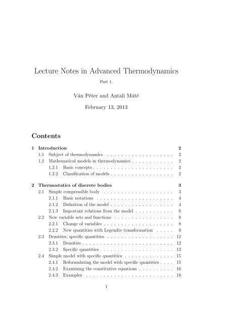
<strong>Lecture</strong> <strong>Notes</strong> <strong>in</strong> <strong>Advanced</strong> <strong>Thermodynamics</strong><br />
Part 1.<br />
Ván Péter and Antali Máté<br />
February 13, 2013<br />
Contents<br />
1 Introduction 2<br />
1.1 Subject of thermodynamics . . . . . . . . . . . . . . . . . . . 2<br />
1.2 Mathematical models <strong>in</strong> thermodynamics . . . . . . . . . . . . 2<br />
1.2.1 Basic concepts . . . . . . . . . . . . . . . . . . . . . . . 2<br />
1.2.2 Classification of models . . . . . . . . . . . . . . . . . . 2<br />
2 Thermostatics of discrete bodies 3<br />
2.1 Simple compressible body . . . . . . . . . . . . . . . . . . . . 3<br />
2.1.1 Basic notations . . . . . . . . . . . . . . . . . . . . . . 4<br />
2.1.2 Def<strong>in</strong>ition of the model . . . . . . . . . . . . . . . . . . 4<br />
2.1.3 Important relations from the model . . . . . . . . . . . 6<br />
2.2 New variable sets and functions . . . . . . . . . . . . . . . . . 8<br />
2.2.1 Change of variables . . . . . . . . . . . . . . . . . . . . 8<br />
2.2.2 New quantities with Legendre transformation . . . . . 9<br />
2.3 Densities, specific quantities . . . . . . . . . . . . . . . . . . . 12<br />
2.3.1 Densities . . . . . . . . . . . . . . . . . . . . . . . . . . 12<br />
2.3.2 Specific quantities . . . . . . . . . . . . . . . . . . . . . 13<br />
2.4 Simple model with specific quantities . . . . . . . . . . . . . . 15<br />
2.4.1 Reformulat<strong>in</strong>g the model with specific quantities . . . . 15<br />
2.4.2 Exam<strong>in</strong><strong>in</strong>g the constitutive equations . . . . . . . . . . 16<br />
2.4.3 Examples . . . . . . . . . . . . . . . . . . . . . . . . . 18<br />
1
1 Introduction<br />
1.1 Subject of thermodynamics<br />
What is the subject of thermodynamics?<br />
– elementary approach: physics of heat, temperature and energy<br />
→ eng<strong>in</strong>eer<strong>in</strong>g advantage: perform<strong>in</strong>g practical calculations of energy<br />
transfer processes (classical thermodynamics course)<br />
– advanced level: general background and framework of macroscopic<br />
physics<br />
→ eng<strong>in</strong>eer<strong>in</strong>g advantage: better understand<strong>in</strong>g of other macroscopic<br />
physics courses (solid mechanics, fluid mechanics, classical thermodynamics,<br />
electrodynamics, physical chemistry)<br />
1.2 Mathematical models <strong>in</strong> thermodynamics<br />
1.2.1 Basic concepts<br />
thermodynamic system : a mathematical abstraction which is used for<br />
modell<strong>in</strong>g a piece of reality, a system is a collection of <strong>in</strong>teract<strong>in</strong>g bodies<br />
thermodynamic body<br />
: the smallest <strong>in</strong>dividual piece of a system<br />
state : the set of all pieces of <strong>in</strong>formation which determ<strong>in</strong>es our whole<br />
knowledge from the system, time and space dependent.<br />
state variables : mathematical objects which are used to represent the<br />
state, they can be numbers, functions, etc. . .<br />
1.2.2 Classification of models<br />
different areas of thermodynamics → different features of state variables<br />
phenomenology - statistics<br />
– phenomenological: state variables are related directly to macroscopic<br />
features of the material<br />
– statistical: state variables are related to the behaviour of the microscopic<br />
particles, and macroscopic features are derived from them by<br />
statistical methods (not covered <strong>in</strong> this subject)<br />
2
thermostatics - thermodynamics<br />
– thermostatics: state variables do not depend on time<br />
(analogy: mechanical statics)<br />
– thermodynamics: state variables can change <strong>in</strong> time<br />
(analogy: mechanical dynamics)<br />
discrete thermodynamics - cont<strong>in</strong>uum thermodynamics<br />
– discrete thermodynamics: state variables are homogeneous<br />
(analogy: mechanics of po<strong>in</strong>t masses and rigid bodies)<br />
– cont<strong>in</strong>uum thermodynamics: state variables are space dependent<br />
(analogy: cont<strong>in</strong>uum mechanics)<br />
2 Thermostatics of discrete bodies<br />
other names:<br />
– thermostatics of homogeneous bodies<br />
– equilibrium ,,thermodynamics”<br />
we can imag<strong>in</strong>e a homogeneous body as a very small amount of material<br />
or a box of material where all the properties are constant <strong>in</strong> space and time<br />
2.1 Simple compressible body<br />
simple compressible body: a thermodynamic body, which can be characterized<br />
<strong>in</strong> equilibrium state by the mass (M), the volume (V ) and the<br />
<strong>in</strong>ternal energy (E)<br />
remarks:<br />
– <strong>in</strong> the follow<strong>in</strong>g ,,body” means this simple compressible body<br />
– this is an appropriate model for thermal and mechanical behaviour of<br />
s<strong>in</strong>gle-component gases<br />
– for other material types (solids, fluids, multi-component gases, radiation,<br />
etc.) or other physical properties (chemical, electrical, etc.) different,<br />
usually more complicated models are used<br />
3
2.1.1 Basic notations<br />
basic state variables: (E, V, M) ∈ (R + ) 3<br />
(they can be chosen <strong>in</strong>tuitively or consider<strong>in</strong>g physical mean<strong>in</strong>g)<br />
state function: an f(E, V, M) : (R + ) 3 → R function which creates a new<br />
state variable from the basic state variables<br />
extensive scal<strong>in</strong>g of a state function (f◦λ)(E, V, M) := f(λE, λV, λM),<br />
where λ is an arbitrary real number<br />
(resizes the system, giv<strong>in</strong>g the value of the state function for a λ times<br />
,,larger” body )<br />
<strong>in</strong>tensive state function: f ◦ λ = f for ∀λ ∈ R<br />
(the state function rema<strong>in</strong>s constant if the body is resized)<br />
extensive state function: f ◦ λ = λ · f for ∀λ ∈ R<br />
(the state function is <strong>in</strong>creas<strong>in</strong>g l<strong>in</strong>early with the resiz<strong>in</strong>g)<br />
remarks:<br />
– the function itself and the value of the function are not strictly dist<strong>in</strong>guished<br />
<strong>in</strong> notation<br />
– <strong>in</strong> the def<strong>in</strong>itions and follow<strong>in</strong>g calculations equal sign (=) between<br />
state functions means equality for all possible (E, V, M) values<br />
– E, V and M can be considered also as extensive state functions, e.g.<br />
E(E, V, M) = E<br />
– the partial derivation of a function can be denoted <strong>in</strong> shorter way:<br />
∂f(E, V, M) ∂f<br />
=:<br />
∂E ∂E ∣ =: ∂ E f<br />
V,M<br />
2.1.2 Def<strong>in</strong>ition of the model<br />
Def<strong>in</strong>ition(discrete thermostatic body):<br />
– a set of ⎧ ⎫<br />
⎨ T (E, V, M) ⎬<br />
p(E, V, M)<br />
⎩ ⎭<br />
µ(E, V, M)<br />
state functions over the (E, V, M) state space<br />
4
– for that there exists a S(E, V, M) state function called entropy, which<br />
has to fulfil the follow<strong>in</strong>g properties:<br />
(P 1 ) (entropy is a potential)<br />
∂S<br />
∂E ∣ = 1<br />
V,M<br />
T ;<br />
∂S<br />
∂V<br />
∣ = p<br />
E,M<br />
T ;<br />
∂S<br />
∂M ∣ = − µ<br />
E,V<br />
T<br />
(1)<br />
(P 2 ) (entropy is <strong>in</strong>creas<strong>in</strong>g with energy)<br />
∂S<br />
∂E ∣ > 0 (2)<br />
V,M<br />
(P 3 ) (entropy is extensive)<br />
S ◦ λ = λ · S (3)<br />
Consequence: The entropy is extensive if and only if there is a specific<br />
entropy function: s(E/M, V/M) = S(E,V,M)<br />
M<br />
(P 4 ) (specific entropy is concave)<br />
D 2 s(e, v) is a negative def<strong>in</strong>ite matrix (4)<br />
Remarks:<br />
– T denotes the temperature, p is for the pressure and µ is called chemical<br />
potential<br />
– T, p and µ functions are called state functions, they correspond to the<br />
thermostatic system, the properties restrict the set of possible constitutive<br />
functions due to physical pr<strong>in</strong>ciples<br />
– the properties are related, but cannot be derived from the laws of thermodynamics,<br />
the dynamical laws have an effect on the structure of the<br />
system even <strong>in</strong> equilibrium state<br />
5
Example: ideal gas<br />
– the well-known equations of the ideal gas (R is the gas constant and c<br />
is the isochoric specific heat, they are real constants):<br />
E = cMT ;<br />
pV = MRT<br />
– from that the state functions are:<br />
T (E, V, M) = E<br />
cM<br />
p(E, V, M) = MRT<br />
V<br />
= RE<br />
cV<br />
– let us choose the chemical potential function as:<br />
µ(E, V, M) = c ln E M + R ln V M<br />
– for these functions an appropriate entropy function:<br />
S(E, V, M) = Mc ln E M + MR ln V M<br />
+ M(c + R)<br />
– it can be easily checked that for c > 0 this entropy function fulfils<br />
properties (P 1 ), (P 2 ) and (P 3 ), for prov<strong>in</strong>g the validity of (P 4 ) a longer<br />
calculation is required<br />
2.1.3 Important relations from the model<br />
Gibbs relation<br />
– the total differential of the entropy function (d can be imag<strong>in</strong>ed as a<br />
very small change <strong>in</strong> the quantity)<br />
dS = ∂S<br />
∂E ∣ dE + ∂S<br />
V,M<br />
∂V ∣ dV + ∂S<br />
E,M<br />
∂M ∣ dM<br />
E,V<br />
– us<strong>in</strong>g the (P 1 ) property:<br />
dS = 1 T dE + p T dV − µ dM (5)<br />
T<br />
– after rearrang<strong>in</strong>g the Gibbs relation is obta<strong>in</strong>ed:<br />
dE = T dS − pdV + µdM (6)<br />
6
<strong>in</strong>tensive property of T ,p and µ:<br />
– let us calculate the resiz<strong>in</strong>g of (5):<br />
dS ◦ λ = 1<br />
T ◦ λ dE ◦ λ + p ◦ λ<br />
T ◦ λ dV ◦ λ − µ ◦ λ<br />
T ◦ λ dM ◦ λ<br />
– E,V ,M are extensive (trivial) and S is extensive too due to property<br />
(P 3 ):<br />
λdS = 1<br />
T ◦ λ λdE + p ◦ λ<br />
T ◦ λ λdV − µ ◦ λ<br />
T ◦ λ λdM<br />
– from that:<br />
∂S<br />
∂E ∣ = 1<br />
V,M<br />
T ◦ λ ;<br />
∂S<br />
∂V<br />
∣ = p ◦ λ<br />
E,M<br />
T ◦ λ ;<br />
– compar<strong>in</strong>g them with property (P 1 ):<br />
∂S<br />
∂M ∣ = − µ ◦ λ<br />
E,V<br />
T ◦ λ<br />
T ◦ λ = T ; p ◦ λ = p; µ ◦ λ = µ (7)<br />
– thus T , p and µ are <strong>in</strong>tensive state functions<br />
Potential relation<br />
– differentiat<strong>in</strong>g property (P 1 ) respect to λ:<br />
(<br />
) (<br />
) (<br />
)<br />
∂S<br />
∂S<br />
∂E ∣ ◦ λ E +<br />
∂S<br />
V,M<br />
∂V ∣ ◦ λ V +<br />
E,M<br />
∂M ∣ ◦ λ M = S<br />
E,V<br />
– us<strong>in</strong>g property (P 1 ):<br />
– us<strong>in</strong>g (7):<br />
1<br />
T ◦ λ E + p ◦ λ<br />
T ◦ λ V − µ ◦ λ<br />
T ◦ λ M = S<br />
1<br />
T E + p T V − µ T M = S<br />
– after rearrang<strong>in</strong>g we get the potential relation:<br />
E = T S − pV + µM (8)<br />
7
2.2 New variable sets and functions<br />
2.2.1 Change of variables<br />
<strong>in</strong>troduction of a new variable<br />
– given a function f(x, y)<br />
– the variable x is changed to z with the substitution x = x(z, y)<br />
– the new function is<br />
ˆf(y, z) := f ( x(y, z), z ) (9)<br />
derivatives respect to the new variable<br />
– (partial) differentiat<strong>in</strong>g (9) respect to z<br />
– rearrang<strong>in</strong>g:<br />
∂ z ˆf|y = ∂ x f| y · ∂ z x| y<br />
∂ x f| y = ∂ z ˆf| y<br />
∂ z x| y<br />
(10)<br />
– special case z = f<br />
∂ x f| y = 1<br />
∂ f x| y<br />
derivatives respect to the rema<strong>in</strong><strong>in</strong>g variable<br />
– (partial) differentiat<strong>in</strong>g (9) respect to y:<br />
– us<strong>in</strong>g (10):<br />
– rearrang<strong>in</strong>g:<br />
– special case z = f<br />
∂ y ˆf|z = ∂ x f| y · ∂ y x| z + ∂ y f| x<br />
∂ y ˆf|z = ∂ z ˆf| y<br />
∂ z x| y<br />
· ∂ y x| z + ∂ y f| x<br />
∂ y f| x = ∂ y ˆf|z − ∂ yx| z<br />
∂ z x| y<br />
· ∂ z ˆf|y (11)<br />
∂ y f| x = −∂ y x| f · ∂ x f| y<br />
8
Example: <strong>in</strong>ternal energy<br />
– let us change the variable space from the standard (E, V, M) to (S, V, M)<br />
– the Gibbs relation rema<strong>in</strong>s valid if we change the T (E, V, M) function<br />
to T (S, V, M) and so on, so the <strong>in</strong>ternal energy is a potential of the<br />
(T, −p, µ) functions:<br />
∂E<br />
∂S<br />
∣ = T ;<br />
V,M<br />
∂E<br />
∂V<br />
∣ = −p;<br />
S,M<br />
∂E<br />
∂M ∣ = µ (12)<br />
S,V<br />
– <strong>in</strong> the previous notations x = E, z = S and the ,,y-s” are V and M<br />
– let f be p(E, V, M), therefore (10) becomes:<br />
∂ E p| V,M = ∂ Sp| V,M<br />
∂ S E| V,M<br />
us<strong>in</strong>g (12):<br />
– now apply<strong>in</strong>g (11):<br />
∂ E p| V,M = ∂ Sp| V,M<br />
T<br />
∂ V p| E,M = ∂ V p| S,M − ∂ V E| S,M<br />
∂ S E| V,M<br />
· ∂ S p| V,M<br />
us<strong>in</strong>g (12):<br />
∂ V p| E,M = ∂ V p| S,M + p T · ∂ Sp| V,M<br />
2.2.2 New quantities with Legendre transformation<br />
<strong>in</strong>troduction of the Legendre transform<br />
– given a function f(x, y)<br />
– the variable x is changed to z with the substitution x = x(z, y)<br />
– the Legendre transform of f(x, y) is g(z, y) which is determ<strong>in</strong>ed by the<br />
follow<strong>in</strong>g two properties:<br />
g(z, y) + x(z, y) · z = f ( x(z, y), y ) (13)<br />
∂ z g| y = −x(z, y) (14)<br />
9
derivatives respect to the new variable<br />
– (partial) differentiat<strong>in</strong>g (13) respect to z<br />
– us<strong>in</strong>g (14):<br />
∂ z g| y + x(z, y) + z · ∂ z x| y = ∂ x f| y · ∂ z x| y<br />
so z can be also considered as a z(x, y) function<br />
z = ∂ x f| y (15)<br />
– from (14) and (15) comes that the derivatives of f and g are <strong>in</strong>verse<br />
functions<br />
– x and z are called conjugated variables<br />
derivatives respect to the variable, that is no transformed<br />
– (partial) differentiat<strong>in</strong>g (13) respect to y:<br />
– us<strong>in</strong>g (15):<br />
∂ y g| z + ∂ y x| z · z = ∂ x f| y · ∂ y x| z + ∂ y f| x<br />
∂ y g| z = ∂ y f| x (16)<br />
the exact equality is valid if the x(z, y) substitution is done on the right<br />
side after the derivation<br />
– thus the Legendre transformation keeps constant the derivatives respect<br />
to the rema<strong>in</strong><strong>in</strong>g variables<br />
example: free energy<br />
– let us start with the f = E(S, V, M) function and x = E, then accord<strong>in</strong>g<br />
to (15):<br />
z = ∂ S E| V,M<br />
due to (12):<br />
z = T<br />
– let the new function be F (T, V, M) and called Helmholtz free energy,<br />
then the formula of the Legendre transformation <strong>in</strong> (13) becomes:<br />
F + ST = E<br />
so the def<strong>in</strong>ition of the free energy is:<br />
F = E − T S (17)<br />
10
– substitut<strong>in</strong>g to the potential relation (8) :<br />
(potential relation for free energy)<br />
– differentiat<strong>in</strong>g (17)<br />
– us<strong>in</strong>g the Gibbs-relation (6):<br />
F = −pV + µM<br />
dF = dE − d(T S) = dE − SdT − T dS<br />
dF = T dS − pdV + µdM − SdT − T dS<br />
(Gibbs relation for free energy)<br />
dF = −SdT − pdV + µdM<br />
– thus after the S ↔ T <strong>in</strong>terchange the free energy is an F (T, V, M) function,<br />
which is a potential of the S(T, V, M), p(T, V, M) and µ(T, V, M)<br />
functions:<br />
∂F<br />
∂T<br />
∣ = −S;<br />
V,M<br />
∂F<br />
∂V<br />
(we can check the validity of (16))<br />
∣ = −p;<br />
T,M<br />
∂F<br />
∂M ∣ = µ<br />
T,V<br />
– it can be checked easily that F is not an extensive function over its<br />
(T, V, M) variable space, but it is extensive if we transform the variables<br />
to the standard (E, V, M) variables<br />
– the whole procedure can be applied similarly to get the enthalpy (H)<br />
and the Gibbs free energy (G), the results can be found <strong>in</strong> the tables,<br />
E, F, H and G are called thermodynamic potentials<br />
quantity def<strong>in</strong>ition potential relation<br />
energy - E = T S − pV + µM<br />
Helmholtz free energy F := E − T S F = −pV + µM<br />
enthalpy H := E + pV H = ST + µM<br />
Gibbs free energy G := E − T S + pV G = µM<br />
Table 1: Important thermodynamic potentials - def<strong>in</strong>itions<br />
11
quantity variables Gibbs relation<br />
energy E(S, V, M) dE = T dS − pdV + µdM<br />
Helmholtz free energy F (T, V, M) dF = −SdT − pdV + µdM<br />
enthalpy H(S, p, M) dH = T dS + V dp + µdM<br />
Gibbs free energy G(T, p, M) dG = −SdT + V dp + µdM<br />
Table 2: Important thermodynamic potentials - variables<br />
2.3 Densities, specific quantities<br />
– the extensive and <strong>in</strong>tensive properties are constra<strong>in</strong>ts<br />
– one of the extensive variables can be elim<strong>in</strong>ated<br />
– it can be useful to choose a reference variable<br />
– usually the volume (densities) and the mass (specific quantities) are<br />
used for reference<br />
2.3.1 Densities<br />
transformation of the basic state variables<br />
– energy density:<br />
ε := E V<br />
– mass density:<br />
ρ := M V<br />
transformation of the state functions<br />
– the (E, V, M) state space can be simplified to (ε, ρ)<br />
– consider<strong>in</strong>g an extensive state function:<br />
( E<br />
ˆf(ε, ρ) := f (ε, 1, ρ) = f<br />
V , 1, M )<br />
= V f ( E<br />
, 1, )<br />
M<br />
V V<br />
=<br />
V V<br />
f(E, V, M)<br />
V<br />
specially:<br />
Ê = ε;<br />
ˆM = ρ<br />
12
– consider<strong>in</strong>g an <strong>in</strong>tensive state function:<br />
( E<br />
ĝ(ε, ρ) := g (ε, 1, ρ) = g<br />
V , 1, M V<br />
)<br />
= g(E, V, M)<br />
– the functions over the new state space (ε, ρ) are <strong>in</strong>tensive functions<br />
potential relation for densities:<br />
– let us divide (8) by V :<br />
E<br />
V = T S V − p + µM V<br />
– us<strong>in</strong>g the def<strong>in</strong>ition of the densities:<br />
Gibbs relation for densities:<br />
– let us substitute the densities to (6):<br />
ε = T s − p + µρ (18)<br />
d(εV ) = T d(sV ) − pdV + µd(ρV )<br />
– us<strong>in</strong>g the derivation rule d(xy) = xdy + ydx:<br />
V dε + εdV = T V ds + T sdV − pdV + µV dρ + µρdV<br />
dV (ε − T s + p − µρ) + V (dε − T ds − µdρ) = 0<br />
– the expression <strong>in</strong> the first bracket is zero due to (18), therefore the<br />
Gibbs relation for densities:<br />
2.3.2 Specific quantities<br />
transformation of the basic state variables<br />
– specific energy:<br />
– specific volume:<br />
dε = T ds + µdρ (19)<br />
e := E M<br />
v := V M<br />
13
transformation of the state functions<br />
– the (E, V, M) state space is simplified to (e, v)<br />
– consider<strong>in</strong>g an extensive state function:<br />
˜f(e, v) := f (e, v, 1) = f<br />
specially:<br />
( E<br />
M , V M , 1 )<br />
= Mf ( E<br />
M , V M , 1)<br />
M<br />
Ẽ = e;<br />
Ṽ = v<br />
=<br />
f(E, V, M)<br />
M<br />
– consider<strong>in</strong>g an <strong>in</strong>tensive state function:<br />
( E<br />
˜g(e, v) := g (e, v, 1) = g<br />
M , V )<br />
M , 1 = g(E, V, M)<br />
– the functions over the state space (e, v) are neither extensive not <strong>in</strong>tensives<br />
potential relation for specific quantities:<br />
– let us divide (8) by M:<br />
– us<strong>in</strong>g the def<strong>in</strong>itions:<br />
E<br />
M = T S M − p V M + µ<br />
e = T s − pv + µ (20)<br />
Gibbs relation for specific quantities:<br />
– let us substitute the specific quantities to (6):<br />
d(eM) = T d(sM) − pd(vM) + µdM<br />
– us<strong>in</strong>g the derivation rule:<br />
Mde + edM = T vds + T sdM − pvdM − pMdv + µdM<br />
dM(ε − T s + pv − µ) + M(de − T ds + pdv) = 0<br />
– from (20) the first bracket equals zero, thus the Gibbs relation:<br />
de = T ds − pdv (21)<br />
14
extensive quantity (A) V M E S F G H<br />
density (A/V ) 1 ρ ε s<br />
specific quantity (A/M) v 1 e s f g h<br />
Table 3: Densities and specific quantities<br />
2.4 Simple model with specific quantities<br />
2.4.1 Reformulat<strong>in</strong>g the model with specific quantities<br />
Def<strong>in</strong>ition(discrete thermostatic body for specific quantities):<br />
– a set of { } T (e, v)<br />
p(e, v)<br />
state functions over the (e, v) state space<br />
– for that there exists a s(e, v) state function called specific entropy, which<br />
has to fulfil the follow<strong>in</strong>g properties:<br />
(B 1 ) (specific entropy is a potential)<br />
∂s<br />
∂e∣ = 1 v<br />
T ; ∂s<br />
∂v ∣ = p<br />
e<br />
T<br />
(22)<br />
(B 2 ) (specific entropy is <strong>in</strong>creas<strong>in</strong>g with energy)<br />
∂s<br />
∂e∣ > 0 (23)<br />
v<br />
remarks:<br />
(B 3 ) (specific entropy is concave)<br />
D 2 s(e, v) is a negative def<strong>in</strong>ite matrix (24)<br />
– if the mass M is constant, this and the previous models are equivalent<br />
– the property correspond<strong>in</strong>g to (P 3 ) is miss<strong>in</strong>g, this property was used<br />
to reduce the three variables to two<br />
– we do not require the complicated extensive and <strong>in</strong>tensive properties<br />
15
2.4.2 Exam<strong>in</strong><strong>in</strong>g the constitutive equations<br />
motivation<br />
– T (e, v) and p(e, v) functions are often given as empirical approximations<br />
– it is useful to check if they fulfil the propertys of thermostatics<br />
– sometimes the propertys can be used to make restrictions to the parameters<br />
of the model<br />
Condition of the potential property of entropy<br />
– if the entropy function is twice differentiable then the mixed second<br />
partial derivatives must be equal<br />
∂ 2 s(e, v)<br />
∂v∂e<br />
= ∂2 s(e, v)<br />
∂e∂v<br />
– us<strong>in</strong>g property (B 1 ):<br />
( )<br />
∂<br />
1<br />
∂v ∣ = ∂ ( )<br />
p(e, v)<br />
e<br />
T (e, v) ∂e∣ v<br />
T (e, v)<br />
(25)<br />
– this condition is useful to check the T and p functions aga<strong>in</strong>st the (B 1 )<br />
property, without calculat<strong>in</strong>g the entropy function<br />
– if (25) is not valid, then there exists no s(e, v) function, if the condition<br />
fulfils, then s exists and the gas described by T and p functions is called<br />
entropic<br />
Condition of the <strong>in</strong>creas<strong>in</strong>g property of entropy<br />
– property (B 2 ) is simple, it requires only<br />
∂s<br />
∂e∣ > 0<br />
v<br />
– if the property (B 1 ) is substituted, a very simple condition is obta<strong>in</strong>ed:<br />
T (e, v) > 0 (26)<br />
therefore the range of the temperature function must be positive<br />
16
Condition of the concave property of specific entropy<br />
– the condition of property (B 2 ) is called thermodynamic stability, which<br />
requires the concavity of the specific entropy function<br />
– the concavity requires that the Hesse-matrix of the specific entropy<br />
function, this D 2 s(e, v) has to be negative def<strong>in</strong>ite (or −D 2 s(e, v) positive<br />
def<strong>in</strong>ite) whenever the function is two times cont<strong>in</strong>uously differentiable<br />
– the positive def<strong>in</strong>iteness of a symmetric matrix can be <strong>in</strong>vestigated by<br />
the Sylvester criteria, a matrix<br />
[<br />
a11 a 12<br />
a 12 a 22<br />
]<br />
is positive def<strong>in</strong>ite if and only if a 11 > 0 and a 11 a 22 − a 2 12 > 0<br />
– apply<strong>in</strong>g to the entropy function:<br />
⎡<br />
= ⎣<br />
]<br />
p<br />
T<br />
Ds = [ ] [<br />
∂ e s| v ∂ v s| e = 1<br />
T<br />
⎡<br />
−D 2 s = ⎣ −∂ ( 1<br />
) ∣ (<br />
∣v<br />
e −∂ 1<br />
) ∣ ⎤<br />
∣e<br />
T<br />
v T<br />
(<br />
−∂ p<br />
) ∣ (<br />
∣v<br />
e −∂ p<br />
) ∣ ⎦<br />
∣e<br />
=<br />
T v T<br />
1<br />
1<br />
∂<br />
T 2 e T | v ∂<br />
T 2 v T | e<br />
− 1 T ∂ ep| v + p<br />
T 2 ∂ e T | v<br />
⎤<br />
− 1 ∂ ⎦<br />
T vp| e + p ∂<br />
T 2 v T | e<br />
– us<strong>in</strong>g the a 11 > 0 condition:<br />
1<br />
T 2 ∂ eT | v > 0<br />
– us<strong>in</strong>g the a 11 a 22 − a 2 12 > 0 condition:<br />
∂ e T | v > 0 (27)<br />
1<br />
T 4 (<br />
∂e T | v (p ∂ v T | e − T ∂ v p| e ) − ∂ v T | e (p ∂ e T | v − T ∂ e p| v ) ) > 0<br />
1 ( )<br />
∂v T |<br />
T 3 e ∂ e p| v − ∂ v p| e ∂ e T | v > 0<br />
− ∂ (<br />
eT | v<br />
∂<br />
T 3 v p| e − ∂ )<br />
vT | e<br />
∂ e p| v > 0<br />
∂ e T | v<br />
17
– the bracket equals to ∂ v p| T because of (11), therefore:<br />
− ∂ eT | v<br />
T 3 ∂ v p| T > 0<br />
– ∂ e T | v is positive due to (27) and T 3 is positive due to (26), thus<br />
∂ v p| T < 0 (28)<br />
– (27) and (28) are a particular example of the le Chatelier-Brown pr<strong>in</strong>ciple.<br />
2.4.3 Examples<br />
ideal gas<br />
– the thermic equation of state:<br />
– the caloric equation of state:<br />
pv = RT<br />
e = cT<br />
– from that the standard state functions:<br />
– the condition of (25):<br />
T (e, v) = e c<br />
p(e, v) = Re<br />
cv<br />
( )<br />
∂<br />
1<br />
∂v ∣ = 0<br />
e<br />
T (e, v)<br />
( )<br />
∂<br />
p(e, v)<br />
∂e∣ = 0<br />
v<br />
T (e, v)<br />
they are equal, hence the ideal gas model is entropic<br />
– the condition (26): because the energy (e) is positive by def<strong>in</strong>ition, the<br />
condition for the positive temperature is:<br />
18<br />
c > 0
– the condition (27):<br />
– the condition (28):<br />
from (26) we get:<br />
∂ e T | v = 1 c > 0<br />
c > 0<br />
p(T, v) = RT<br />
v<br />
∂ v p| T = − RT<br />
v 2<br />
R > 0<br />
– therefore if c > 0 and R > 0 then an ideal gas fulfils the properties of<br />
thermostatics<br />
van der Waals gas<br />
– the termic equation of state is:<br />
– the caloric equation of state is:<br />
p = RT<br />
v − b − a v 2<br />
T = e c + a cv<br />
– therefore the standard state functions:<br />
– the condition (25):<br />
p(e, v) =<br />
p<br />
T =<br />
T (e, v) = e c + a cv<br />
Re<br />
c(v − b) + Ra<br />
cv(v − b) − a v 2<br />
1<br />
T =<br />
c<br />
e + a v<br />
R<br />
v − b − a v · 2<br />
e + a v<br />
it can be checked that<br />
( )<br />
∂<br />
1<br />
∂v ∣ = ∂ ( )<br />
p(e, v)<br />
e<br />
T (e, v) ∂e∣ =<br />
v<br />
T (e, v)<br />
therefore the van der Waals gas model is entropic<br />
19<br />
c<br />
ac<br />
(ev + a) 2
– the condition (26):<br />
e<br />
c + a cv > 0<br />
if c > 0 then ev > −a, if c < 0 then ev < a<br />
– the condition (27):<br />
∂ e T | v = 1 c > 0<br />
c > 0<br />
– the condition (28):<br />
∂ v p| T = −<br />
RT<br />
(v − b) + 2a<br />
2 v < 0 3<br />
– Therefore the van der Waals gas body fulfils (B 2 ) and (B 3 ) properties<br />
for a given doma<strong>in</strong> of (e, v) restricted by the parameters.<br />
20


