There's more to volatility than volume - Santa Fe Institute

More documents

Recommendations

Info

V. LONG-MEMORY There is mounting evidence that volatility is a long-memory process (Ding, Granger, and Engle 1993, Breidt, Crato and de Lima 1993, Harvey 1993, Andersen et al. 2001). A longmemory process is a random process with an autocorrelation function that is not integrable. This typically happens when the autocorrelation function decays asymptotically as a power law of the form τ −γ with γ < 1. The existence of long-memory is important because it implies that values from the distant past have a significant effect on the present and that the stochastic process lacks a typical time scale. A stochastic process that is build out of a sum whose increments have long-memory has anomalous diffusion, i.e. the variance grows as τ 2H , where H > 0.5, and H is the Hurst exponent, which is defined below. Statistical averages of long-memory processes converge slowly. Plerou et al. (2000) demonstrated that the number of transactions in NYSE stocks is a long-memory process. This led them to conjecture that fluctuations in the number of transactions are the proximate cause of long-memory in volatility. This hypothesis makes sense in light of the fact that either long-memory or sufficiently fat tails in fluctuations in transaction frequencies are sufficient to create long-memory in volatility (Deo, Hsieh, and Hurvich 2005). However, our results so far in this paper suggests caution – just because it is possible to create long-memory with this mechanism does not mean it is the dominant mechanism – there may be multiple sources of long-memory. If there are two long memory processes with autocorrelation exponents γ 1 and γ 2 , if γ 1 < γ 2 the long-memory of process one will dominate that of process two, since for large values of τ C 1 (τ) ≫ C 2 (τ). We will see that this is the case here – the long-memory caused by fluctuations in volume and number of transactions is dominated by long-memory caused by other factors. We investigate the long-memory of volatility by computing the Hurst exponent H. For a random process whose second moment is finite and whose autocorrelation function asymptotically decays as a power law τ −γ with 0 < γ < 1, the Hurst exponent is H = 1 − γ/2. A process has long memory if 1/2 < H < 1. We compute the Hurst exponent rather than working directly with the autocorrelation function because it is better behaved statistically. We compute the Hurst exponent using the DFA method (Peng et al. 1994). The time series {x(t)} is first integrated to give X(t) = ∑ t i=1 x(i). For a data set with n points, X(t) is then broken into K disjoint sets k = 1, . . . , K of size L ≈ n/K. A polynomial Y k,L of order m is then fit for each set k using a least squares regression. For a given value of L let D(L) be the root mean square deviation of the data from the polynomials averaged over the K sets, i.e. D(L) = (1/K ∑ k,i(X(i) − Y k,L (x(i)) 2 ) 1/2 . The Hurst exponent is formally defined as H = lim L→∞ lim n→∞ log D(L)/ log L. In practice, with a data set of finite n the Hurst exponent is measured by regressing log D(L) against log L over a region with L min < L < n/4. H is the slope of the regression. To test the hypothesis that the number of transactions drives the long-memory of volatility we compute the Hurst exponent of the real time volatility, H(ν), and compare it to the Hurst exponent of the volatility in transaction time, H(ν θ ), and the Hurst exponent in shuffled transaction real time, H(˜ν θ ). If the long-memory of transaction time is the dominant cause of volatility then we should see that H(ν) ≈ H(˜ν θ ), due to the fact that ˜ν preserves the number of transactions in each 15 minute interval, and we should also see that H(ν) > H(ν θ ), due to the fact that ν θ holds the number of transactions constant in each interval, so it should not display as much clustered volatility. We illustrate the scaling diagrams used to compute these three Hurst exponents for the LSE stock Astrazeneca in
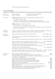
FIG. 8: Computation of Hurst exponent of volatility for the LSE stock Astrazeneca. The logarithm of the average variance D(L) is plotted against the scale log L. The Hurst exponent is the slope. This is done for real time volatility ν (black circles), transaction time volatility ν θ (red crosses), and shuffled transaction real time volatility ˜ν θ (blue triangles). The slopes in real time and transaction time are essentially the same, but the slope for shuffled transaction real time is lower, implying that transaction fluctuations are not the dominant cause of long-memory in volatility. Figure 8. This figure does not support the conclusion that transaction time fluctuations are the proximate cause of volatility. We find H(ν) ≈ 0.70 ± 0.07, H(ν θ ) ≈ 0.70 ± 0.07, and H(˜ν θ ) ≈ 0.59 ± 0.03. Thus for Astrazenca it seems the opposite is true, i.e. H(ν) ≈ H(ν θ ) and H(ν) > H(˜ν θ ). While it is true that H(˜ν θ ) > 0.5, which means that fluctuations in transaction frequency contribute to long-memory, the fact that H(ν θ ) > H(˜ν θ ) means that this is dominated by even stronger long-memory effects that are caused by other factors. Note that the quoted error bars for H as based on the assumption that the data are normal and IID, and are thus much too optimistic. For a long-memory process such as this the relative error scales as n (H−1) rather than n −1/2 , and estimating accurate error bars is difficult. The only known procedure is the variance plot method (Beran, 1992), which is not very reliable and is tedious to implement. This drives us to make a cross-sectional test, where the consistency of the results and their dependence on other factors will make the statistical significance quite clear. To test the consistency of our results above we compute Hurst exponents for all the stocks in each of our three data sets. In addition, to test whether fluctuations in volume are important, we also compute the Hurst exponents of volatility in volume time, H(ν v ) and in shuffled volume real time, H(˜ν v ). The results are shown in Figure 9, where we plot the Hurst exponents for H(ν θ ), H(˜ν θ ), H(ν v ), and H(˜ν v ) against the real time volatility H(ν) for each stock in each data set. Whereas the Hurst exponents in volume and transaction time cluster along the identity line, the Hurst exponents for shuffled real time are further away from the identity line and are consistently lower in value. This is seen at a glance in the figure by the fact that the solid marks are clustered along the identity line whereas the open marks are scattered away from it. The results are quite consistent – out of the 60 cases
Page 1 and 2: There’s more to volatility than v
Page 3 and 4: themselves. Plerou et al. divide th
Page 5 and 6: privately, there are no published q
Page 7 and 8: B. Volatility in transaction time T
Page 9 and 10: FIG. 3: An illustration of the rela
Page 11 and 12: the majority of variation in volati
Page 13 and 14: FIG. 5: Cumulative distribution of
Page 15 and 16: FIG. 6: Cumulative distribution of
Page 17: FIG. 7: Test of the theory of Gabai
Page 21 and 22: volatility market a b d (×100) R 2
Page 23 and 24: of the work in Farmer et al. (2004)
Page 25: [17] A. R. Gallant, P. E. Rossi, an

There's more to volatility than volume - Santa Fe Institute

You also want an ePaper? Increase the reach of your titles

Delete template?

Save as template?