The Economy at Full Employment - Pearson

Chapter 

7 THE 

ECONOMY AT 

FULL EMPLOYMENT* 

Key Concepts 

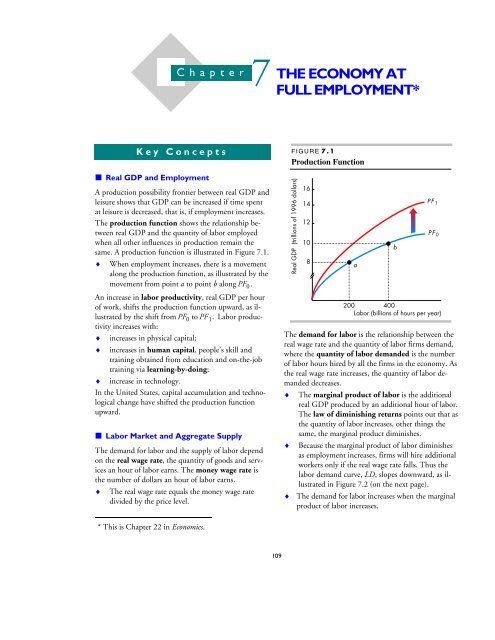
FIGURE 7.1 

Production Function 

Real GDP and Employment 

A production possibility frontier between real GDP and 

leisure shows that GDP can be increased if time spent 

at leisure is decreased, that is, if employment increases. 

The production function shows the relationship between 

real GDP and the quantity of labor employed 

when all other influences in production remain the 

same. A production function is illustrated in Figure 7.1. 

♦ When employment increases, there is a movement 

along the production function, as illustrated by the 

movement from point a to point b along PF 0 . 

An increase in labor productivity, real GDP per hour 

of work, shifts the production function upward, as illustrated 

by the shift from PF 0 to PF 1. 

Labor productivity 

increases with: 

♦ increases in physical capital; 

♦ increases in human capital, people’s skill and 

training obtained from education and on-the-job 

training via learning-by-doing; 

♦ increase in technology. 

In the United States, capital accumulation and technological 

change have shifted the production function 

upward. 

Labor Market and Aggregate Supply 

The demand for labor and the supply of labor depend 

on the real wage rate, the quantity of goods and services 

an hour of labor earns. The money wage rate is 

the number of dollars an hour of labor earns. 

♦ The real wage rate equals the money wage rate 

divided by the price level. 

Real GDP (trillions of 1996 dollars) 

16 

14 

12 

10 

8 

a 

PF 1 

PF 0 

200 400 

Labor (billions of hours per year) 

The demand for labor is the relationship between the 

real wage rate and the quantity of labor firms demand, 

where the quantity of labor demanded is the number 

of labor hours hired by all the firms in the economy. As 

the real wage rate increases, the quantity of labor demanded 

decreases. 

♦ 

The marginal product of labor is the additional 

real GDP produced by an additional hour of labor. 

The law of diminishing returns points out that as 

the quantity of labor increases, other things the 

same, the marginal product diminishes. 

♦ Because the marginal product of labor diminishes 

as employment increases, firms will hire additional 

workers only if the real wage rate falls. Thus the 

labor demand curve, LD, slopes downward, as illustrated 

in Figure 7.2 (on the next page). 

♦ The demand for labor increases when the marginal 

product of labor increases. 

b 

* This is Chapter 22 in Economics. 

109

110 

CHAPTER 7 (22) 

FIGURE 7.2 

The Labor Market 

Real wage rate (1996 dollars per hour) 

35 

LS 

LD 

200 


The supply of labor is the relationship between the 

quantity of labor supplied and the real wage rate when 

all other influences on work plans remain the same. 

♦ The labor supply curve, LS, slopes upward, as illustrated 

in Figure 7.2, because higher real wage 

rates increase the amount of goods and services that 

can be purchased for an hour’s work. 

In Figure 7.2 the equilibrium real wage rate is $35 per 

hour and equilibrium employment is 200 billion hours. 

♦ The equilibrium quantity of employment from the 

labor market and the production function determine 

potential GDP. The long-run aggregate 

supply curve, LAS, is the relationship between the 

quantity of real GDP supplied and the price level 

when real GDP equals potential GDP. The LAS 

curve is vertical at potential GDP. 

♦ In the short run, the labor market can depart from 

full employment. The short-run aggregate supply 

curve, SAS, is the relationship between the quantity 

of real GDP supplied and the price level when the 

money wage rate and potential GDP remain constant. 

The SAS curve is upward sloping. 

♦ If the price level rises and the money wage does not 

change, the real wage falls. Firms hire more workers, 

real GDP increases and the economy moves 

along the SAS curve. A shortage of labor results so 

that the money wage rate rises. Eventually the real 

wage rate returns to its equilibrium and GDP again 

equals potential GDP. 

Changes in Potential GDP 

Real GDP increases if the economy recovers from a 

recession or it potential GDP increases. Potential GDP 

increases if the population increases or if labor productivity 

increases. 

♦ An increase in population increases the supply of 

labor so that the labor supply curve shifts rightward. 

The production function does not shift. Employment 

increases and the economy moves along 

its (unchanged) production function to a higher 

level of potential GDP. 

♦ An increase in labor productivity (because of an 

increase in physical capital, human capital, or technology) 

shifts the production function upward and 

increases the demand for labor. Employment increases 

because of the increase in demand for labor. 

Potential GDP increases because employment increases 

and because the production function has 

shifted upward. 

In the United States, over the last twenty years, the 

population increased, thereby increasing the supply of 

labor. The demand for labor increased because the 

capital stock increased and because technology advanced. 

Both these last two factors increased productivity 

and thus shifted the production function upward. 

So potential GDP has increased because equilibrium 

employment has increased and because the production 

function has shifted upward. 

Unemployment at Full Employment 

Two factors help explain why unemployment is always 

present even at full employment (when the unemployment 

rate equals the natural rate of unemployment): 

♦ Job search — the activity of looking for an acceptable 

vacant job. The length of time spent searching, 

and hence the natural rate of unemployment, increases 

when more young people enter the labor 

market; when unemployment compensation payments 

become more generous; and when structural 

change in the economy increases. 

♦ Job rationing — paying workers an aboveequilibrium 

wage rate and then rationing jobs by 

some method. Jobs can be rationed because of efficiency 

wages (paying a higher wage rate to increase 

productivity) or because of a minimum wage law 

(which sets the lowest legal wage a firm can pay) 

that prevents some workers from finding jobs.

THE ECONOMY AT FULL EMPLOYMENT 111 

Helpful Hints 

1. FROM THE LABOR MARKET TO POTENTIAL GDP : 

The production function stands between the labor 

market and the aggregate output market. The equilibrium 

level of employment is determined in the 

labor market and then the production function indicates 

how much output results from that level of 

employment. 

The labor market functions like the “typical” supply 

and demand markets you studied in Chapter 3. 

Everything you learned there about how to use the 

supply and demand model applies to the labor 

market in this chapter. In particular, the key difference 

between shifts in a curve versus movements 

along a curve continues to apply: Changes in the 

real wage rate create movements along the labor 

demand and labor supply curves while other relevant 

factors shift these curves. 

2. PRODUCTION FUNCTION : The production function 

graphically illustrates the relationship between 

the amount of labor employment and the level of 

real GDP. 

In the next chapters you will meet a similar concept, 

the “productivity function”. The productivity 

function relates output per hour of work to capital 

per hour of work. Graphically, the productivity 

function appears similar to the production function. 

The productivity function is related to the 

production function but it is not the same. Thoroughly 

study the production function now so that 

you are not confused between the two when you 

study the productivity function. 

Questions 

True/False and Explain 


11. If the production possibilities frontier does not 

shift, real GDP can be increased only if leisure is 

increased. 

12. An increase in employment causes a movement 

along the production function. 

13. Labor productivity increases when the amount of 

the nation’s human capital increases. 

14. Learning-by-doing increases the nation’s physical 

capital. 

15. In the United States, there have been movements 

along the U.S. production function but no shifts in 

the function. 


16. The demand for labor curve is downward sloping. 

17. As more workers are employed, the marginal product 

of labor increases. 

18. A rise in the real wage rate increases the quantity of 

labor supplied. 

19. When employment equals the equilibrium quantity, 

the economy is on its LAS curve. 


10. An increase in the demand for labor raises the real 

wage rate. 

11. An increase in the demand for labor increases potential 

GDP. 

12. An increase in the nation’s physical capital stock 

decreases the demand for labor. 

13. An increase in labor productivity shifts the production 

function downward and decreases the quantity 

of employment. 

14. Since 1980 in the United States, the supply of labor 

has increased more than the demand for labor. 


15. When the unemployment rate equals the natural 

rate, there is no job search. 

16. An increase in unemployment compensation will 

decrease job search. 

17. Efficiency wages can be a cause of unemployment. 

Multiple Choice 


11. The production possibilities frontier between real 

GDP and leisure 

a. shifts inward when the capital stock increases 

because unemployment rises. 

b. shows that increasing leisure will decrease real 

GDP. 

c. shifts if employment increases. 

d. All of the above answers are correct.

112 


12. Which of the following shifts the nation’s production 

function upward? 

a. An increase in employment. 

b. A decrease in employment. 

c. An increase in human capital. 

d. A decrease in human capital. 

13. A movement along the production function with no 

shift in the production function is created by 

a. changes in the amount of physical capital. 

b. changes in the amount of human capital. 

c. advances in technology. 

d. changes in employment. 

14. Between 1980 and 2001, the U.S. production function 

shifted ____ and the quantity of labor hours 

____. 

a. upward; increased 

b. upward; decreased 

c. downward; increased 

d. downward; decreased 


15. The money wage rate is $10 per hour and the price 

level is 100. If the price level rises to 200 and the 

money wage rate does not change, what happens to 

the real wage rate? 

a. The real wage rate doubles. 

b. The real wage rate rises, but does not double. 

c. The real wage rate does not change. 

d. The real wage rate falls. 

16. Five workers produce total output of $200; six 

workers produce total output of $222. The marginal 

product of the sixth worker equals 

a. $40. 

b. $37. 

c. $22. 

d. None of the above answers is correct. 

17. The demand curve for labor is downward sloping 

because the 

a. marginal product of labor diminishes as more 

workers are employed. 

b. supply curve of labor is upward sloping. 

c. demand curve shifts when capital increases. 

d. None of the above answers are correct because 

the demand curve for labor is upward sloping. 

18. As the real wage rate increases, the quantity of labor 

supplied increases 

a. only because people already working increase the 

quantity of labor they supply. 

b. only because the higher wage rate increases labor 

force participation. 

c. because people already working increase the 

quantity of labor they supply and because the 

higher wage rate increases labor force participation. 

d. None of the above answers is correct because an 

increase in the real wage rate decreases the quantity 

of labor supplied. 

19. A rise in the real wage rate 

a. shifts the labor demand curve rightward. 

b. shifts the labor demand curve leftward. 

c. shifts the labor supply curve leftward. 

d. does not shift the labor demand or labor supply 

curve. 

10. If the economy is at full employment, the 

a. entire population is employed. 

b. entire labor force is employed. 

c. long-run aggregate supply curve is upward sloping. 

d. the quantity of labor supplied equals the quantity 

of labor demanded. 

11. At potential GDP, 

a. the labor market is in equilibrium, with the 

quantity of labor demanded equal to the quantity 

supplied. 

b. there is no necessary relationship between the 

quantity of labor demanded and the quantity 

supplied. 

c. the real wage has adjusted so that it equals the 

money wage. 

d. the real wage rate must be rising because otherwise 

people will not work. 


12. An increase in population shifts the 

a. labor demand curve rightward. 

b. labor demand curve leftward. 

c. labor supply curve rightward. 

d. labor supply curve leftward.


13. An increase in productivity from new technology 

shifts the production function ____ and shifts the 

demand for labor curve ____. 

a. upward; rightward 

b. upward; leftward 

c. downward; rightward 

d. downward; leftward 

14. An increase in the demand for labor ____ the real 

wage and ____ the quantity of employment. 

a. raises; increases 

b. raises; decreases 

c. lowers; increases 

d. lowers; decreases 

15. Which of the following will NOT increase labor 

productivity? 

a. An increase in physical capital. 

b. An increase in human capital. 

c. An increase in employment. 

d. An advance in technology. 

16. In the United States, from 1981 to 2001, the demand 

for labor has 

a. increased more than the supply of labor has 

increased. 

b. increased less than the supply of labor increased. 

c. increased while the supply of labor has decreased. 

d. decreased while the supply of labor has increased 

17. The demand for labor and the supply of labor are 

both increasing over time, but the demand for labor 

is increasing at a faster rate. Over time, therefore, 

you would expect to see the real wage rate ____ and 

employment ____. 

a. rise; increase 

b. rise; decrease 

c. fall; increase 

d. fall; decrease 


18. An increase in unemployment compensation payments 

will 

a. decrease the extent of search unemployment. 

b. lead to more job rationing. 

c. decrease the extent of demographic change. 

d. increase the length of time a worker searches for 

a job. 

19. Which of the following is a reason that jobs might 

be rationed? 

a. Efficiency wages 

b. Equilibrium real wage rate. 

c. The vertical LAS curve. 

d. An increase in the demand for labor 

20. An efficiency wage refers to 

a. workers being paid wages below the equilibrium 

wage rate in order to increase the economy’s 

efficiency. 

b. wages being set to generate the efficient level of 

unemployment. 

c. workers being paid wages above the equilibrium 

wage rate in order to increase their productivity. 

d. None of the above. 

21. Suppose that the real wage rate is above the equilibrium 

real wage rate. Then the quantity demanded of 

labor ___ the quantity supplied of labor and there 

____ unemployment. 

a. is more than; is 

b. is more than; is not 

c. is less than; is not 

d. is less than; is 

Short Answer Problems 

1. What is the connection between the production 

possibilities frontier showing the relationship between 

leisure and real GDP and the production 

function showing the relationship between employment 

and real GDP? 

2. a. What does diminishing returns mean? 

b. Moving along a production function, why does 

the marginal product of labor diminish as employment 

increases? 

3. Why is the marginal product of labor curve the 

same as the labor demand curve? What does this 

equality imply for the slope of the labor demand 

curve? 

4. a. What is the real wage rate? How does it differ 

from the money rate? How is the real wage rate 

constructed? 

b. Why does the supply of labor depend on the 

real wage rate rather than the money wage rate?

114 


FIGURE 7.3 

Short Answer Problem 5 

FIGURE 7.4 



25 

20 

15 

10 

5 

LS 

LD 


17 

15 

13 

11 

10 

PF 

0 

50 

100 150 200 250 


200 300 400 


5. In Figure 7.3 what is the equilibrium real wage 

rate? Illustrate a real wage rate at which jobs are rationed. 

Indicate the amount of unemployment. 

6. What can account for job rationing? 

7. Suppose that new technology shifts the production 

function upward and increases labor productivity. 

Using Figures 7.4 and 7.5, show what happens in 

both. Does the equilibrium quantity of employment 

rise or fall? Does real GDP increase or decrease? 

You’re the Teacher 

1. “Look, I really studied this chapter, but why 

bother? I mean, I thought we were going to be 

learning about stuff like money, and recessions, and 

stuff like that. I know that unemployment is important, 

but why do we bother to study unemployment 

at full employment?” It is undoubtedly 

good that your friend has been studying this chapter, 

but it undoubtedly would be better if your 

friend understood why this chapter is important. 

Can you help your friend grasp this key point? 

FIGURE 7.5 



LS 

21 

14 

7 

LD 

100 200 300 400 

Labor (billions of hours per year)


True/False Answers 

Answers 


11. F Increasing leisure decreases employment and 

hence decreases real GDP. 

12. T An increase in employment causes a movement 

along the production function to a higher level 

of real GDP. 

13. T When productivity increases, the nation’s production 

function shifts upward. 

14. F Learning-by-doing increases human capital, not 

physical capital. 

15. F The U.S. production function has shifted upward 

because of increases in capital and advances 

in technology. 


16. T The demand for labor curve is downward sloping 

because the marginal product of labor diminishes 

as more workers are employed. 

17. F As more workers are employed, the marginal 

product diminishes. 

18. T If the real wage rate rises, more workers enter the 

labor force and workers already in the labor 

force supply more hours of work. 

19. T Equilibrium employment is full employment, 

which means the economy is at potential GDP 

on its LAS curve. 


10. T An increase in the demand for labor raises both 

the real wage rate and employment. 

11. T Because an increase in the demand for labor 

increases employment, it also increases potential 

GDP. 

12. F An increase in capital raises the marginal product 

of labor, which increases the demand for labor. 

13. F An increase in productivity shifts the production 

function upward and increases the quantity of 

employment. 

14. F The demand for labor has increased by more 

than the supply of labor and, as a result, the real 

wage has risen. 


15. F Job search always exists. 

16. F An increase in unemployment compensation 

creates more job search and hence increases unemployment. 

17. T When wages are set above the equilibrium level, 

unemployment results. 

Multiple Choice Answers 


11. b If leisure increases, people are spending less time 

at work. As a result, real GDP decreases. 

12. c Changes in employment, answers (a) and (b), 

create movements along the production function. 

An increase in human capital shifts the 

production function upward. 

13. d As the previous answer pointed out, changes in 

employment create a movement along the production 

function. Changes in other relevant 

factors shift the production function. 

14. a The production function shifted upward because 

of increases in productivity. 


15. d The real wage rate equals the money wage rate 

divided by the price level so when the price level 

rises and the money wage rate does not change, 

the real wage rate falls 

16. c The marginal product of labor equals the change 

in output divided by the change in employment, 

or, in this case, ($222 – $200)/(6 – 5) = $22. 

17. a The demand for labor curve is the same as the 

marginal product of labor curve. 

18. c For both reasons given in the answer, the supply 

of labor curve is upward sloping, indicating that 

an increase in the real wage rate increases the 

quantity of labor supplied. 

19. d A change in the real wage rate creates a movement 

along the labor demand and labor supply 

curves but does not shift either curve. 

10. d When the labor market is in equilibrium, the 

economy is at full employment. 

11. a When the labor market is in equilibrium — the 

quantity of labor supplied equals the quantity of 

labor demanded — the economy is producing its 

potential GDP.

116 



12. c With more people, the supply of labor increases. 

13. a The increase in productivity increases the marginal 

product of labor, which shifts the demand 

for labor curve rightward. 

14. a As Figure 7.6 illustrates, the increase in the demand 

for labor is reflected in the rightward shift 

in the demand curve from LD 0 to LD 1 . The 

wage rate rises from $10 an hour to $15 and the 

level of employment increases from 100 billion 

hours to 150 billion. This answer demonstrates 

how an increase in productivity and the resulting 

increase in the demand for labor (the last question) 

results in a higher real wage rate. 

FIGURE 7.6 

Multiple Choice Question 14 


25 

20 

15 

10 

5 

0 

50 

LS 

LD 0 

LD 1 

100 150 200 250 


15. c By itself, an increase in employment will create a 

movement along the production function to a 

lower level of productivity. 

16. a Because the demand for labor has increased 

more than the supply of labor, the real wage rate 

has risen. 

17. a The situation outlined in the question is what 

occurred in the United States, so in the United 

States employment and the real wage rate have 

increased. 


18. d Unemployment compensation payments reduce 

the cost of being unemployed, so an increase in 

these payments makes unemployed workers 

more willing to search for longer periods of time 

to find better jobs. 

19. a Efficiency wages and the minimum wage both 

can lead to job rationing. 

20. c Answer (c) is the definition of an efficiency 

wage. 

21. d With the real wage rate above the equilibrium 

wage rate, there are workers who cannot find 

jobs and these workers are unemployed. 

Answers to Short Answer Problems 

1. The production possibilities frontier and the production 

function are basically opposite sides of the 

same coin. 

The production possibilities frontier shows that if 

leisure is decreased — so that employment is increased 

— then real GDP increases. Because of increasing 

opportunity cost, the production 

possibilities frontier also shows that as more additional 

time is spent in employment, the additional 

GDP that results diminishes. 

The production function shows similar results. The 

production function demonstrates that if employment 

increases, real GDP increases. Because of diminishing 

returns, the production function also 

shows that as employment increases, the additional 

GDP that results diminishes. 

2. a. Diminishing returns means that as the quantity 

of labor increases, the additional GDP that results 

diminishes. In other words, the 1,000,001st 

hour of labor by itself creates less additional 

GDP than does the 1,000,000th hour of labor. 

b. Moving along a production function, the marginal 

product of labor diminishes because along 

the production function the amount of the 

capital stock and technology are constant. Thus 

additional labor must work with the same number 

of factories, assembly lines, and so forth. In 

this situation, an added worker might not create 

much additional output because the assembly 

lines, machine tools, and so forth are already efficiently 

stocked with enough workers. 

3. The marginal product of labor is the same as the 

labor demand curve because firms want to earn the 

maximum possible profit. When a firm is considering 

hiring another worker, the firm looks at two 

factors: How much it costs to hire the worker and


how much the worker adds to the firm’s output. If 

the worker adds more to the firm’s output than it 

costs to hire the worker, the firm will employ the 

worker. (Conversely, if it costs more to hire the 

worker than the worker adds to output, the firm 

will not hire the worker.) 

The cost of hiring another worker is the real wage 

rate. And, the amount of output that the worker 

produces is the marginal product of labor. If the 

marginal product exceeds the real wage rate, the 

firm hires the worker because it is profitable. As the 

firm hires more and more workers, the marginal 

product of labor diminishes. But, as long as the 

marginal product exceeds the real wage rate, the 

firm hires the workers because by so doing the firm 

raises its profit. Eventually the firm hires enough 

workers so that the marginal product of an additional 

worker just equals the real wage. The firm 

will hire this worker but will hire no more workers 

because for all additional workers the marginal 

product of labor would be less than the real wage 

rate. So the quantity of workers that the firm hires is 

determined by the marginal product of labor curve, 

so that the quantity hired is given by the marginal 

product of labor curve. But the quantity of workers 

the firm hires is the same as the quantity it demands, 

so therefore the marginal product of labor 

curve is the same as the labor demand curve. 

4. a. The real wage rate shows the quantity of goods 

and services that can be purchased with an 

hour’s labor. The money wage rate is the quantity 

of money received for an hour’s labor. The 

real wage rate is defined as the money wage rate 

divided by the price level. 

b. The supply of labor depends on the real wage 

rate because workers are interested in what they 

can buy in exchange for their work. The money 

wage rate just shows the number of dollar bills 

that the worker will receive for an hour’s labor. 

But the worker is concerned with what can be 

purchased with these dollar bills, which is what 

the real wage rate indicates. 

5. In Figure 7.7 the equilibrium wage rate is $15 an 

hour. Any wage rate higher than the equilibrium 

wage rate creates some job rationing. For instance, 

at the wage rate of $20 an hour, the demand for labor 

is only 100 billion hours of labor, yet at this 

wage rate 200 billion hours of labor are supplied. At 

FIGURE 7.7 



25 

20 

15 

10 

5 

0 

50 

LS 

LD 

100 150 200 250 


this wage rate unemployment is 100 billion hours of 

labor. 

More generally, at any wage rate, the extent of unemployment 

equals the difference between the 

quantity of labor supplied and the quantity demanded. 

6. Two factors can account for job rationing: efficiency 

wages and the minimum wage. 

Efficiency wages occur when firms pay aboveequilibrium 

wage rates to increase their workers’ 

productivity. Firms might pay a wage rate that exceeds 

the equilibrium wage rate knowing that, although 

the higher wage rate increases their costs, 

this effect is more than offset by the higher productivity 

of the workers receiving the higher wage rate. 

Finally, the minimum wage might be at a level that 

is above the equilibrium wage rate. In this case the 

quantity of labor demanded is less than that supplied, 

and jobs are rationed because not everyone 

who wants to work at the going (minimum) wage 

rate can find employment. 

7. Start with the production function, illustrated in 

Figure 7.8 (on the next page). The upward shift and 

increase in productivity are illustrated. (Your diagram 

does not need to look exactly like what is illustrated, 

but the production function must shift 

upward and become steeper.) 

The key feature of this change is that labor productivity 

increased, so the change increases the demand 

for labor. Hence in Figure 7.9, the demand for

118 


FIGURE 7.8 


FIGURE 7.9 



15 

13 

11 

9 

7 

a 

b 

PF 1 

PF 0 


21 

14 

7 

LS 

LD 0 

LD 1 

200 300 400 


100 

200 300 400 


labor curve has shifted rightward, from LD 0 to 

LD 1 . (Your figure does not need to look exactly 

like Figure 7.9, as long as the labor demand curve 

has shifted rightward.) As a result, the equilibrium 

quantity of employment increases, to 300 billion 

hours, and the equilibrium real wage rate rises, to 

$21 per hour in the figure. 

GDP changes for two reasons: First, the production 

function has shifted upward, so even if employment 

did not change, GDP would increase. But, employment 

does increase. Thus as Figure 7.8 demonstrates, 

GDP increases from $7 trillion to $12 

trillion as the economy moves from point a on production 

function PF0 

to point b on production 

function PF 1 . 

You’re the Teacher 

1. “Well the things you mentioned, money, recessions, 

and so on are important and when I flip through 

the book I see that we’ll get to them a little later in 

the class. But they are not the only really important 

macroeconomic topics. I mean, one of the really 

important topics is economic growth, how rapidly 

our economy grows. And it’s this topic that this 

chapter is concerned about. 

“Look, here’s how I see it. We want to know how 

fast our economy can grow and what we can do to 

make sure that it grows at the best speed possible, 

right? Well, economic growth basically depends on 

two things: the resources our nation has and the 

technology we can use. Well, one of the most important 

resources is labor and this chapter is focusing 

on that. This chapter helped me understand 

what factors change the equilibrium amount of labor, 

like the productivity growth. I mean, productivity 

has to be important because it not only 

increases the demand for labor and so increases the 

amount of labor that will be employed, but it also 

increases our real wages. 

“And look, I’ve been talking with our teacher again 

and our teacher said that this chapter and the next 

two concentrate on economic growth. This chapter 

talks about one resource, labor. The next covers another 

resource, capital. And the one after that puts 

all this together with a discussion of technology. So, 

this chapter is part of an important group. 

“So, don’t get upset because we aren’t talking about 

money or recessions or other stuff yet. Be patient; 

we’ll get there. But in the meantime let’s settle back 

and learn all about economic growth!”


Chapter Quiz 

11. A nation’s production function shifts upward if 

a. employment increases. 

b. employment decreases. 

c. human capital increases. 

d. physical capital decreases. 

12. Diminishing marginal product of labor means that 

a. the supply of labor curve is upward sloping so 

that a higher real wage increases the quantity of 

labor supplied. 

b. as more labor is employed, GDP decreases. 

c. the demand for labor curve is upward sloping. 

d. as more labor is employed, the additional 

amount of GDP produced diminishes. 

13. If the money wage rate rises and the price level does 

not change, the real wage rate 

a. increase. 

b. do not change. 

c. decrease. 

d. probably change, but without knowledge of the 

labor demand and labor supply, it is impossible 

to tell the direction. 

14. When the economy producing more than potential 

GDP, 

a. the labor market is in equilibrium. 

b. the real wage rate is below the equilibrium real 


c. the real wage rate is above the equilibrium real 


d. None of the above answers are correct. 

15. If the demand for labor increases, the equilibrium 

quantity of employment ___ and potential GDP 

____. 

a. increases; increases 

b. increases; decreases 

c. decreases; increases 

d. decreases; decreases 

16. In the United States, from 1981 to 2001, which of 

the following accurately describes what occurred? 

a. Employment increased because population 

growth increased the labor supply and technological 

change increased the demand for labor. 

b. Employment decreased because population 

growth lead to increased amounts of unemployment 

and technological change decreased the 

demand for labor. 

c. Employment grew because population growth 

increased the supply of labor but the real wage 

fell because technological change decreased the 

demand for labor. 

d. None of the above answers are correct. 

17. The demand for labor is ____ sloped; the supply of 

labor curve is ____ sloped. 

a. positively; positively 

b. positively; negatively 

c. negatively; positively 

d. negatively; negatively 

18. If the supply of labor increases more than the demand 

for labor, then the real wage rate ____ and 

the level of employment ____. 

a. rises; increases 

b. rises; decreases 

c. falls; increases 

d. falls; decreases 

19. Job search occurs 

a. only when the supply of labor increases. 

b. only when the quantity of labor demanded exceeds 

the quantity of labor supplied. 

c. only when the quantity of labor supplied exceeds 

the quantity of labor demanded. 

d. at all times. 

10. Job search increases if 

a. the minimum wage falls. 

b. efficiency wages are lowered. 

c. unemployment compensation payments increase. 

d. the demand for labor increases. 

The answers for this Chapter Quiz are on page 309

120

The Economy at Full Employment - Pearson

You also want an ePaper? Increase the reach of your titles

Delete template?

Save as template?