Central California Ozone Study (CCOS) - Desert Research Institute
Central California Ozone Study (CCOS) - Desert Research Institute
Central California Ozone Study (CCOS) - Desert Research Institute

You also want an ePaper? Increase the reach of your titles
YUMPU automatically turns print PDFs into web optimized ePapers that Google loves.
<strong>Central</strong> <strong>California</strong> <strong>Ozone</strong> <strong>Study</strong> (<strong>CCOS</strong>)<br />
Volume II:<br />
Field Operations Plan<br />
Version 2<br />
May 31, 2000
<strong>CCOS</strong> Field Operations Plan Version 2: 5/31/00<br />
<strong>Central</strong> <strong>California</strong> <strong>Ozone</strong> <strong>Study</strong> – Volume II<br />
Field Operations Plan<br />
Prepared by:<br />
Eric Fujita, Robert Keislar, William Stockwell, Saffet Tanrikulu and Andrew Ranzieri<br />
Dan Freeman, John Bowen and Richard Tropp Planning and Technical Support Division<br />
Division of Atmospheric Science<br />
<strong>California</strong> Air Resources Board<br />
<strong>Desert</strong> <strong>Research</strong> <strong>Institute</strong><br />
2020 L Street<br />
2215 Raggio Parkway Sacramento, CA 95812<br />
Reno, NV 89512<br />
www.arb.ca.gov<br />
www.arb.ca.gov/ccaqs/ccos/ccos.htm<br />
The <strong>CCOS</strong> Plan was prepared with extensive input from the <strong>CCOS</strong> Field <strong>Study</strong> Participants, Technical<br />
Committee, Scientific Advisory Work Group, Meteorological Work Group, and Emission Inventory<br />
Coordination Group.<br />
Technical Committee<br />
(Planning Subcommittee)<br />
Andrew Ranzieri, <strong>California</strong> Air Resources Board<br />
Saffet Tanrikulu, <strong>California</strong> Air Resources Board<br />
Rob DeMandel, Bay Area AQMD<br />
Bruce Katayama, Sacramento Metropolitan AQMD<br />
Evan Shipp, San Joaquin Valley Unified APCD<br />
Phil Roth, Envair<br />
Jim Sweet, San Joaquin Valley Unified APCD<br />
Brigette Tollstrup, Sacramento Metropolitan AQMD<br />
Steve Ziman, Chevron <strong>Research</strong> and Technology<br />
Scientific Advisory Work Group<br />
Dan Chang, University of <strong>California</strong>, Davis<br />
Dennis Fitz, UCR, CE-CERT<br />
Robert Harley, University of <strong>California</strong>, Berkeley<br />
Mike Kleeman, University of <strong>California</strong>, Davis<br />
Gail Tonnesen, University of <strong>California</strong>, Riverside<br />
Meteorological Work Group<br />
Saffet Tanrikulu, <strong>California</strong> Air Resources Board<br />
Bob Keislar, <strong>Desert</strong> <strong>Research</strong> <strong>Institute</strong><br />
David Fairley, Bay Area AQMD<br />
Tom Umeda, Bay Area AQMD<br />
Evan Shipp, San Joaquin Valley Unified APCD<br />
Steve Gouze, <strong>California</strong> Air Resources Board<br />
Bruce Katayama, Sacramento Metropolitan AQMD<br />
Brigette Tollstrup, Sacramento Metropolitan AQMD<br />
Bob Noon, Monterey Bay Unified AQMD<br />
Emission Inventory Coordination Group<br />
Linda Murchison, <strong>California</strong> Air Resources Board<br />
Dale Shimp, <strong>California</strong> Air Resources Board<br />
Cheryl Taylor, <strong>California</strong> Air Resources Board<br />
Dennis Wade, <strong>California</strong> Air Resources Board<br />
Michael Benjamin, <strong>California</strong> Air Resources Board<br />
Phil Martien, Bay Area AQMD<br />
Toch Mangat, Bay Area AQMD<br />
Bruce Katayama, Sacramento Metropolitan AQMD<br />
Brigette Tollstrup, Sacramento Metropolitan AQMD<br />
Hazel Hoffmann, San Joaquin Valley Unified APCD<br />
Dave Jones, San Joaquin Valley Unified APCD<br />
Tom Jordon, San Joaquin Valley Unified APCD<br />
Scott Nestor, San Joaquin Valley Unified APCD<br />
Stephen Shaw, San Joaquin Valley Unified APCD<br />
Gretchen Bennett, Northern Sierra AQMD<br />
Dick Johnson, Placer County APCD<br />
Tom Roemer, San Luis Obispo County APCD<br />
Larry Green, Yolo-Solano AQMD<br />
Nancy O’Connor, Yolo-Solano AQMD<br />
Dave Smith, Yolo-Solano AQMD<br />
Gordon Garry, Sacramento Area CoG<br />
Guido Franco, <strong>California</strong> Energy Commission<br />
Morris Goldberg, U.S. EPA<br />
ii
<strong>CCOS</strong> Field Operations Plan Version 2: 5/31/00<br />
FIELD STUDY PARTICIPANTS<br />
Technical Coordination<br />
Don McNerny, <strong>California</strong> Air Resources Board<br />
Andrew Ranzieri, <strong>California</strong> Air Resources Board<br />
Saffet Tanrikulu, <strong>California</strong> Air Resources Board<br />
Eric Fujita, <strong>Desert</strong> <strong>Research</strong> <strong>Institute</strong><br />
Field Management and Facilities<br />
Eric Fujita, <strong>Desert</strong> <strong>Research</strong> <strong>Institute</strong><br />
Dan Freeman, <strong>Desert</strong> <strong>Research</strong> <strong>Institute</strong><br />
Chuck McDade, ENSR<br />
Dave Wright, AVES/ATC Associates, Inc.<br />
Episode Forecast<br />
Saffet Tanrikulu, <strong>California</strong> Air Resources Board<br />
Evan Shipp, San Joaquin Valley Unified APCD<br />
Avi Okin, Bay Area AQMD<br />
John Ching, Sacramento Metropolitan AQMD<br />
Bob Keislar, <strong>Desert</strong> <strong>Research</strong> <strong>Institute</strong><br />
Supplemental Surface Air Quality Operations<br />
John Bowen, <strong>Desert</strong> <strong>Research</strong> <strong>Institute</strong><br />
Richard Tropp, <strong>Desert</strong> <strong>Research</strong> <strong>Institute</strong><br />
Bill Coulombe, <strong>Desert</strong> <strong>Research</strong> <strong>Institute</strong><br />
Bill Stockwell, <strong>Desert</strong> <strong>Research</strong> <strong>Institute</strong><br />
Dennis Fitz, UC Riverside, CE-CERT<br />
Don Lehrman, T&B Systems<br />
Robert Harley, UC Berkeley<br />
Nitrogen Species Measurements<br />
Dennis Fitz, UC Riverside, CE-CERT<br />
Kurt Burmiller, UC Riverside, CE-CERT<br />
John Collins, UC Riverside, CE-CERT<br />
Claudia Sauer, UC Riverside, CE-CERT<br />
John Pisano, UC Riverside, CE-CERT<br />
Susanne Hering, Aerosol Dynamics, Inc.<br />
Airborne Measurements<br />
Don Blumenthal, Sonoma Technology, Inc.<br />
Jerry Anderson, Sonoma Technology, Inc.<br />
John Carroll, UC Davis<br />
Alan Dixon, UC Davis<br />
Roger Tanner, Tennessee Valley Authority<br />
Ralph Valente, Tennessee Valley Authority<br />
Rich Barchet, Pacific Northwest National Laboratory<br />
Shiyuan Zhnog, PNNL<br />
Leonard Barrie, PNNL<br />
Quality Assurance Audits<br />
Dave Bush, Parsons Engineering Science<br />
Bob Baxter, Parsons Engineering Science<br />
Dave Wright, AVES/ATC Associates, Inc.<br />
Lin Linsey, Northwest <strong>Research</strong> Assoc., Inc.<br />
Mike Miguel, <strong>California</strong> Air Resources Board<br />
Don Fitzell, <strong>California</strong> Air Resources Board<br />
Avi Okin, Bay Area AQMD<br />
Data Management and Evaluation<br />
Greg O’Brien, <strong>California</strong> Air Resources Board<br />
Liz Niccum, T&B Systems<br />
Eric Fujita, <strong>Desert</strong> <strong>Research</strong> <strong>Institute</strong><br />
Sponsoring Organizations<br />
<strong>California</strong> Air Resources Board<br />
<strong>California</strong> Energy Commission<br />
Bay Area Air Quality Management District<br />
Mendocino County Air Pollution Control District<br />
Sacramento Metropolitan AQMD<br />
San Joaquin Unified Air Pollution Control District<br />
San Luis Obispo Air Pollution Control District<br />
Western States Petroleum Association<br />
Volatile Organic Compound Measurements<br />
Barbara Zielinska, <strong>Desert</strong> <strong>Research</strong> <strong>Institute</strong><br />
John Sagebiel, <strong>Desert</strong> <strong>Research</strong> <strong>Institute</strong><br />
Wendy Goliff, <strong>Desert</strong> <strong>Research</strong> <strong>Institute</strong><br />
Rei Rasmussen, Biospheric <strong>Research</strong> Corporation<br />
Kochy Fung, AtmAA<br />
Supplemental Meteorological Measurements<br />
Bill Neff, NOAA<br />
Clark King, NOAA<br />
Jerry Crescenti, NOAA<br />
Tom Strong, NOAA<br />
Tim Dye, Sonoma Technology, Inc<br />
Don Lehrman, T&B Systems<br />
Jay Rosenthal, U.S. Navy<br />
iii
<strong>CCOS</strong> Field Operations Plan Version 2: 5/31/00<br />
TABLE OF CONTENTS<br />
Page<br />
List of Tables ............................................................................................................................... vii<br />
List of Figures ................................................................................................................................ix<br />
1.0 INTRODUCTION ............................................................................................................... 1-1<br />
1.1 Basis for the <strong>Study</strong> Design.......................................................................................... 1-2<br />
1.2 Technical Objectives................................................................................................... 1-5<br />
1.3 Field <strong>Study</strong> Design Guidelines.................................................................................... 1-9<br />
1.4 Guide to the <strong>CCOS</strong> Field Operations Plan................................................................ 1-11<br />
2.0 FIELD MEASUREMENTS ................................................................................................ 2-1<br />
2.1 Geographic Scope ....................................................................................................... 2-1<br />
2.2 <strong>Study</strong> Period................................................................................................................ 2-1<br />
2.3 Existing Monitoring Networks.................................................................................... 2-3<br />
2.3.1 Criteria Pollutant Air Monitoring Stations...................................................... 2-4<br />
2.3.2 Photochemical Assessment Monitoring Stations ............................................ 2-4<br />
2.3.3 Surface Meteorological Networks................................................................... 2-8<br />
2.3.4 Solar Radiation Measurements...................................................................... 2-11<br />
2.4 <strong>CCOS</strong> Surface Air Quality and Meteorological Monitoring Network...................... 2-12<br />
2.4.1 Network Design and Measurements.............................................................. 2-13<br />
2.4.2 Complementary Measurement Programs ...................................................... 2-23<br />
2.4.3 Equipment Procurement and Checkout......................................................... 2-25<br />
2.4.4 Facilities Installation ..................................................................................... 2-26<br />
2.4.5 Equipment Installation and Calibrations ....................................................... 2-26<br />
2.4.6 Site Operations .............................................................................................. 2-27<br />
2.4.7 Maintenance and Repair................................................................................ 2-32<br />
2.4.8 Data Acquisition and Review........................................................................ 2-33<br />
2.5 <strong>CCOS</strong> Ground-Based Aloft Air Quality and Meteorological Measurements ........... 2-35<br />
2.5.1 Continuous Upper-Air Meteorological Measurements ................................. 2-35<br />
2.5.2 Radiosondes/<strong>Ozone</strong>sondes............................................................................ 2-43<br />
2.5.3 <strong>Ozone</strong> LIDAR ............................................................................................... 2-44<br />
2.6 In-Situ Aircraft Measurements.................................................................................. 2-44<br />
2.6.1 Overview of Flight Plans............................................................................... 2-46<br />
2.6.2 University of <strong>California</strong>, Davis Cessna 182 (UCD #1 and UCD #2)............ 2-51<br />
2.6.3 Sonoma Technology Inc. Piper Aztec........................................................... 2-52<br />
2.6.4 Sonoma Technology Inc. Cessna 182 ........................................................... 2-52<br />
2.6.5 Pacific Northwest National Laboratory Gulfstream 159 (G-1)..................... 2-63<br />
2.6.6 Tennessee Valley Authority (TVA) Twin Otter............................................ 2-71<br />
2.6.7 VOC Sample Collection Methods and Protocols.......................................... 2-72<br />
2.6.8 Intercomparison Flights................................................................................. 2-73<br />
iv
<strong>CCOS</strong> Field Operations Plan Version 2: 5/31/00<br />
TABLE OF CONTENTS (cont.)<br />
Page<br />
3.0 FORECAST AND IOP DECISION PROTOCOL.............................................................. 3-1<br />
3.1 <strong>Ozone</strong> Episodes and Transport Scenarios of Interest.................................................. 3-1<br />
3.2 Forecast Protocol......................................................................................................... 3-3<br />
3.3 IOP Decision-Making Protocol................................................................................... 3-6<br />
4.0 QUALITY ASSURANCE................................................................................................... 4-1<br />
4.1 Quality Assurance Organization, Responsibilities, and Tasks.................................... 4-2<br />
4.2 Schedule of QA Activity ............................................................................................. 4-3<br />
4.3 Audit Standards And Certification.............................................................................. 4-4<br />
4.4 System Audit Procedures ............................................................................................ 4-9<br />
4.4.1 Radar Profilers and RASS............................................................................... 4-9<br />
4.4.2 Sodars............................................................................................................ 4-10<br />
4.4.3 Surface Meteorological Measurements ......................................................... 4-11<br />
4.4.4 Rawinsondes.................................................................................................. 4-11<br />
4.4.5 NMOC and Carbonyl Samplers .................................................................... 4-11<br />
4.4.6 Continuous Gas/Particulate Analyzers.......................................................... 4-12<br />
4.4.7 Additional Samplers and Analyzers.............................................................. 4-13<br />
4.4.8 Data Processing/Management ....................................................................... 4-13<br />
4.4.9 Laboratories................................................................................................... 4-14<br />
4.5 Performance Audit Procedures.................................................................................. 4-15<br />
4.5.1 Radar Profilers .............................................................................................. 4-15<br />
4.5.2 RASS............................................................................................................. 4-15<br />
4.5.3 Sodars............................................................................................................ 4-16<br />
4.5.4 Surface Meteorological Measurements ......................................................... 4-16<br />
4.5.5 General Performance Audit Procedures for Air Samplers............................ 4-18<br />
4.5.6 NMOC and Carbonyl Samplers .................................................................... 4-19<br />
4.5.7 Continuous Air Quality Samplers ................................................................. 4-19<br />
4.5.8 VOC Laboratory Audits ................................................................................ 4-23<br />
4.6 Approaches To Problem Resolution And Verification Of Corrections .................... 4-23<br />
5.0 DATA MANAGEMENT AND VALIDATION................................................................. 5-1<br />
5.1 Data Specifications...................................................................................................... 5-1<br />
5.1.1 Parameter Codes.............................................................................................. 5-2<br />
5.1.2 Investigator Codes........................................................................................... 5-2<br />
5.1.3 Measurement Codes ........................................................................................ 5-2<br />
5.1.4 Methods Codes................................................................................................ 5-2<br />
5.2 Data Validation Levels................................................................................................ 5-2<br />
5.3 Validation Flags .......................................................................................................... 5-4<br />
5.4 Data Transmittal.......................................................................................................... 5-4<br />
5.4.1 Adherence to Specifications............................................................................ 5-5<br />
5.4.2 Transmittal Files ............................................................................................. 5-5<br />
v
<strong>CCOS</strong> Field Operations Plan Version 2: 5/31/00<br />
TABLE OF CONTENTS (cont.)<br />
Page<br />
5.4.3 Transmittal File Naming Convention.............................................................. 5-5<br />
5.4.4 Transmittal Files Content ................................................................................ 5-6<br />
5.5 Internet Server and Internet Access ............................................................................ 5-6<br />
6.0 EMISSION INVENTORY DEVELOPMENT AND EVALUATION............................... 6-1<br />
6.1 “Fast Track” and Final Modeling Inventory Development Process ........................... 6-1<br />
6.2 Requirements for Quality Control and Quality Assurance of Emission Inventory..... 6-2<br />
6.3 Proposed Contractor Studies for Emission Inventory Development........................... 6-2<br />
6.3.1 Day-Specific Traffic Count Information......................................................... 6-2<br />
6.3.2 Gridding of Area Source Emissions................................................................ 6-3<br />
6.3.3 Integration of Transportation Data for <strong>CCOS</strong> Domain and Run DTIM for<br />
Entire Modeling Domain................................................................................. 6-3<br />
6.3.4 Biogenic Emission Model Expansion ............................................................. 6-3<br />
6.3.5 Small District Assistance ................................................................................ 6-4<br />
6-4 Schedule for Emission Inventory Development.......................................................... 6-4<br />
7.0 MANAGEMENT, SCHEDULE, AND BUDGET.............................................................. 7-1<br />
7.1 <strong>CCOS</strong> Management Structure..................................................................................... 7-1<br />
7.1.1 Policy Committee............................................................................................ 7-1<br />
7.1.2 Technical Committee ...................................................................................... 7-2<br />
7.1.3 Principal Investigators..................................................................................... 7-2<br />
7.1.4 Field <strong>Study</strong> Management Team....................................................................... 7-3<br />
7.1.5 Meteorological Working Group and Forecast Team....................................... 7-3<br />
7.1.6 Field Manager ................................................................................................. 7-3<br />
7.1.7 Field Facilities Coordinator............................................................................. 7-4<br />
7.1.8 Quality Assurance Manager............................................................................ 7-4<br />
7.1.9 Measurement Investigators ............................................................................. 7-5<br />
7.1.10 Emissions Inventory Working Group.............................................................. 7-6<br />
7.1.11 Data Manager .................................................................................................. 7-6<br />
7.1.12 Data Analysis and Modeling Investigators ..................................................... 7-7<br />
7.2 Schedule ...................................................................................................................... 7-8<br />
7.3 Budget......................................................................................................................... 7-8<br />
8.0 REFERENCES.................................................................................................................... 8-1<br />
APPENDICES<br />
A. <strong>CCOS</strong> Phone and Internet Directory .................................................................................. A-1<br />
B. List of Air Montoring Stations in <strong>Central</strong> <strong>California</strong> ..........................................................B-1<br />
C. Decriptions of <strong>CCOS</strong> Measurement Methods .....................................................................C-1<br />
D. Supplemental Air Quality Site Descriptions and Installation Information......................... D-1<br />
vi
<strong>CCOS</strong> Field Operations Plan Version 2: 5/31/00<br />
Table No.<br />
LIST OF TABLES<br />
Page No.<br />
Table 2.3-1 PAMS Target Species.......................................................................................... 2-6<br />
Table 2.3-2 PAMS Sites in the <strong>CCOS</strong> Area............................................................................ 2-7<br />
Table 2.4-1 <strong>CCOS</strong> Supplemental Surface Measurements .................................................... 2-14<br />
Table 2.4-2<br />
Table 2.4-3a<br />
Table 2.4-3b<br />
Table 2.4-3c<br />
Table 2.4-4<br />
Detection Limits, Ranges, and Averaging Times for <strong>CCOS</strong> Supplemental<br />
Measurements .................................................................................................... 2-15<br />
Supplemental Surface Air Quality and Meteorological Measurement Sites<br />
in the Sacramento Valley and Northern Sierra Nevada Foothills...................... 2-16<br />
Supplemental Surface Air Quality and Meteorological Measurement Sites<br />
in the San Francisco Bay Area........................................................................... 2-17<br />
Supplemental Surface Air Quality and Meteorological Measurement Sites<br />
in the San Joaquin Valley, <strong>Central</strong> Sierra Nevada Foothills and South<br />
<strong>Central</strong> Coast ..................................................................................................... 2-18<br />
Primary, calibration, performance test and performance audit standards and<br />
frequencies for <strong>CCOS</strong> measurements ................................................................ 2-28<br />
Table 2.4-5 <strong>CCOS</strong> Supplemental Site Operations Tasks and Operators............................... 2-31<br />
Table 2.5-1 Upper Air Meteorological Measurements for <strong>CCOS</strong>......................................... 2-36<br />
Table 2.6-1 A-1) Aztec Coastal Flight Plan, Santa Rosa to Paso Robles, Morning --<br />
Takeoff 0600 PDT For Episode Types 1 and 2................................................. 2-53<br />
Table 2.6-2 A-2) Aztec Coastal Flight Plan, Paso Robles to Santa Rosa, Afternoon --<br />
Takeoff 1300 PDT For Episode Types 1 and 2.................................................. 2-54<br />
Table 2.6-3<br />
Table 2.6-4<br />
Table 2.6-5<br />
Table 2.6-6<br />
Table 2.6-7<br />
Table 2.6-8<br />
Table 2.6-9<br />
A-3) Aztec Northern Boundry Flight Plan, Santa Rosa to Modesto,<br />
Morning -- Takeoff 0530 PDT For Episode Types 2 and 3............................. 2-55<br />
A-4) Aztec Northern San Joaquin Valley Flight Plan, Santa Rosa to<br />
Modesto, Morning -- Takeoff 0530 PDT For Episode Types 2 and 3............. 2-56<br />
A-5) Aztec Northern San Joaquin Valley Flight Plan, Modesto to Santa<br />
Rosa, Afternoon – Takeoff 1300 PDT ............................................................... 2-57<br />
C-1) Cessna San Joaquin Valley Flight Plan, Bakersfield to Modesto,<br />
Morning -- Takeoff 0600 PDT For Episode Types 1 and 2.............................. 2-58<br />
C-2) Cessna San Joaquin Valley Flight Plan, Modesto to Bakersfield,<br />
Afternoon -- Takeoff 1330 PDT For Episode Types 1 and 2............................. 2-59<br />
C-3) Cessna Modified San Joaquin Valley Flight Plan, Modesto to<br />
Bakersfield, Afternoon -- Takeoff 1330 PDT For Episode Types 2 and 3........ 2-60<br />
C-4) Cessna Southern San Joaquin Valley Flight Plan, Bakersfield to Paso<br />
Robles, Morning -- Takeoff 0530 PDT For Episode Types 2 and 3.................. 2-61<br />
vii
<strong>CCOS</strong> Field Operations Plan Version 2: 5/31/00<br />
Table No.<br />
Table 2.6-10<br />
LIST OF TABLES (cont.)<br />
Page No.<br />
C-5) Cessna Southern San Joaquin Valley Flight Plan, Paso Robles to<br />
Bakerfield, Afternoon – Takeoff 1330 PDT...................................................... 2-62<br />
Table 2.6-11. Fresno area morning flight with low-level passes or spirals over key way<br />
points.................................................................................................................. 2-64<br />
Table 2.6.12 Fresno area afternoon flight with circuits above and within mixed layer.......... 2-65<br />
Table 2.6-13. Western In-Flow Boundary flights..................................................................... 2-68<br />
Table 2.6-14. PSC-FAT ferry flight ......................................................................................... 2-69<br />
Table 2.6-15. FAT-PSC ferry flgiht ......................................................................................... 2-70<br />
Table 2.6-16. Schedule of G-1 Activity in <strong>CCOS</strong>.................................................................... 2-70<br />
Table 3.3-1 Chronology of Daily Forecast and IOP decisions................................................ 3-8<br />
Table 4.2-1<br />
Specifies the audit schedule for the ARB QA audit teams<br />
(Van A and B)...................................................................................................... 4-4<br />
Table 4.2-1 ARB Audit Schedule – Van A............................................................................. 4-5<br />
Table 4.2-2 ARB Audit Schedule – Van B ............................................................................. 4-6<br />
Table 4.5-1. Summary of Meteorolgy Audit Methods and Criteria....................................... 4-24<br />
Table 4.5-2. Linear Regression Criteria ................................................................................. 4-26<br />
Table 5-1-1. Validation Flags ................................................................................................... 5-4<br />
Table 5-2-1. FTP Transmittal file names.................................................................................. 5-6<br />
Table 6.4-1 1999 Baseline Annual Average Emission Inventory Development..................... 6-5<br />
Table 6.4-2 2000 Baseline Modeling Inventory Development ............................................. 6-10<br />
Table 7.2-1 <strong>CCOS</strong> Schedule of Milestones............................................................................. 7-9<br />
Table 7.3-1 <strong>CCOS</strong> Contracts and Other Costs ..................................................................... 7-10<br />
Table 7.3-2<br />
Equipment and Supplies from <strong>CCOS</strong> Equipment Budget and<br />
Contingency Fund .............................................................................................. 7-11<br />
Table 7.3-3 Equipment from <strong>CCOS</strong> Contracts and CRPAQS Equipment Budget............... 7-12<br />
viii
<strong>CCOS</strong> Field Operations Plan Version 2: 5/31/00<br />
Figure No.<br />
LIST OF FIGURES<br />
Page No.<br />
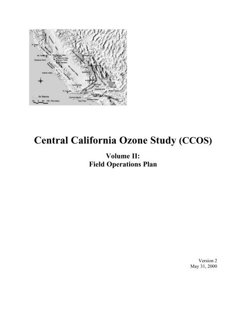
Figure 2.1-1 Overall study domain with major landmarks, mountains and passes. ................. 2-2<br />
Figure 2.3-1.<br />
Figure 2.3-2.<br />
<strong>Central</strong> <strong>California</strong> surface meteorological networks and measurement<br />
locations. ............................................................................................................. 2-9<br />
Surface meteorological observables measured in the combined central<br />
<strong>California</strong> meteorological network..................................................................... 2-10<br />
Figure 2.4-1. Existing routine O3 and NOx monitoring sites.................................................. 2-19<br />
Figure 2.4-2.<br />
Figure 2.5-1.<br />
<strong>CCOS</strong> supplemental air quality and meteorological monitoring sites and<br />
Photochemical Assessment Monitoring Stations ............................................... 2-20<br />
Upper air meteorological measurements during the summer campaign,<br />
including annual average study sites and NEXRAD (WSR-88D) profilers...... 2-41<br />
Figure 2.5-2. Upper air meteorological measurement network indicating operating agency. .2-42<br />
Figure 2.6-1. Morning flight paths for <strong>CCOS</strong> IOPs................................................................. 2-48<br />
Figure 2.6-2. Afternoon flight paths for <strong>CCOS</strong> IOPs ............................................................. 2-49<br />
Figure 2.6-3. Afternoon flight path for post <strong>CCOS</strong> IOPs........................................................ 2-50<br />
Figure 2.6-4.<br />
Figure 2.6-5.<br />
Fresno area flight patterns for morning flights with low-level passes or<br />
spirals at key way points (left) and afternoon flights with circuits above<br />
and within mixed layer (right)............................................................................ 2-66<br />
Schematic representation of the flight patterns for the morning and afternoon<br />
western in-flow boundary flights. Fresno Air Terminal is at the far right,<br />
Monterey near center.......................................................................................... 2-67<br />
Figure 2.6-6. Flight patterns for ferry flights between Pasco, WA (PSC) and Fresno ............ 2-71<br />
ix
<strong>CCOS</strong> Field Operations Plan Version 2: 5/31/00<br />
1.0 INTRODUCTION<br />
The <strong>Central</strong> <strong>California</strong> <strong>Ozone</strong> <strong>Study</strong> (<strong>CCOS</strong>) is a multi-year program of meteorological<br />
and air quality monitoring, emission inventory development, data analysis, and air quality<br />
simulation modeling. The goals of <strong>CCOS</strong> are to: 1) obtain suitable air quality, meteorological<br />
and emission databases to evaluate and improve air quality models for representing urban and<br />
regional-scale ozone episodes in central and northern <strong>California</strong> to meet the regulatory<br />
requirements for the state 1-hour and pending federal 8-hour ozone standards; 2) determine the<br />
contributions of transport and locally generated ozone and the relative benefits of hydrocarbon<br />
and nitrogen oxides emission controls in upwind areas; and 3) assess the relative contributions of<br />
ozone generated from emissions in one air basin to state and federal exceedances in neighboring<br />
air basins. The modeling domain for <strong>CCOS</strong> covers all of central <strong>California</strong> and most of northern<br />
<strong>California</strong>, extending from the Pacific Ocean to east of the Sierra Nevada Mountains and from<br />
Redding to the Mojave <strong>Desert</strong>. The selection of this study area reflects the regional nature of the<br />
state 1-hour and federal 8-hour ozone exceedances, increasing urbanization of traditionally rural<br />
areas, and a need to include all of the major flow features that affect air quality in central<br />
<strong>California</strong>. The <strong>CCOS</strong> field measurement program will be conducted in the summer of 2000 in<br />
conjunction with the <strong>California</strong> Regional PM 10 /PM 2.5 Air Quality <strong>Study</strong> (CRPAQS), a major<br />
study of the origin, nature and extent of excessive levels of fine particles in central <strong>California</strong><br />
(Watson et al., 1998).<br />
The <strong>CCOS</strong> is a large-scale program involving many sponsors and participants. Three<br />
entities are involved in the overall management of the <strong>Study</strong>. The San Joaquin Valleywide Air<br />
Pollution <strong>Study</strong> Agency, a joint powers agency (JPA) formed by the nine counties in the Valley,<br />
directs the contracting aspects of the <strong>Study</strong>. A Policy Committee comprised of four voting<br />
blocks: State, local, and federal government, and the private sector, provides guidance on the<br />
<strong>Study</strong> objectives and funding levels. The Policy Committee approves all proposal requests,<br />
contracts and reports and is responsible for fund raising. A Technical Committee parallels the<br />
Policy Committee in membership and provides overall technical guidance on proposal requests,<br />
direction and progress of work, contract work statements, and reviews of all technical reports<br />
produced from the study. The technical committee comprises staff from the <strong>California</strong> Air<br />
Resources Board, U.S. Environmental Protection Agency, the <strong>California</strong> Energy Commission,<br />
local air pollution control agencies, and industry, with technical input from a consortium of<br />
university researchers in the University of <strong>California</strong> System and the <strong>Desert</strong> <strong>Research</strong> <strong>Institute</strong><br />
(DRI). On a day-to-day basis, the <strong>California</strong> Air Resources Board is responsible for management<br />
of the <strong>Study</strong>.<br />
The <strong>CCOS</strong> plan consists of a field study plan (Volume I) and this field operations plan<br />
(Volume II). These documents correspond to the two phases of the planning process for <strong>CCOS</strong> 1 .<br />
The <strong>CCOS</strong> field study plan (Version 3: 11/24/99) is a product of regular meetings of the <strong>CCOS</strong><br />
Technical Committee and Working Groups over a six-month period and input from local air<br />
pollution control districts, academia, and industry reviewers on two earlier versions of the plan<br />
1 Parallel efforts are also underway to develop a broad conceptual model of ozone formation in central <strong>California</strong><br />
based on San Joaquin Valley Air Quality <strong>Study</strong> and Atmospheric Utility Signatures, Predictions and Experiments<br />
Regional Model Adaptation Program (SARMAP) and other relevant studies and a “comprehensive” study plan that<br />
addresses the long-term research needs related to the ozone problem in central <strong>California</strong> (Roth, 1999a and 1999b).<br />
Chapter 1: INTRODUCTION 1-1
<strong>CCOS</strong> Field Operations Plan Version 2: 5/31/00<br />
(released on 6/11/99 and 9/7/99). The field study plan describes the goals and technical<br />
objectives to be addressed by the study, and describes alternative experimental, modeling, and<br />
data analysis approaches for addressing the study objectives. It presents a summary of the current<br />
knowledge of meteorology, emissions, and chemical and physical processes that affect the<br />
formation and accumulation of ozone in northern and central <strong>California</strong>. It also reviews the<br />
results from prior SAQM 2 modeling by ARB, and identifies the remaining uncertainties and their<br />
implications for the design of the <strong>CCOS</strong> field measurement program. The plan describes<br />
requirements for the modeling and data analysis approaches that are proposed to address <strong>CCOS</strong><br />
technical objectives and specifies measurements for modeling and data analysis. It considers the<br />
merits of alternative measurement approaches and explains the rationale and criteria for<br />
measurement decisions. The field study plan is available in PDF format on the study web site at<br />
http://www.arb.ca.gov/ccaqs/ccos/ccos.htm.<br />
The field study plan served as the basis for contracts with measurement groups and for<br />
developing the field operations plan for the summer 2000 field study. This field operations plan<br />
specifies the details of the field measurement program that will allow the field study plan to be<br />
executed with available resources. It identifies measurement locations, observables, and<br />
monitoring methods, specifies data management and reporting conventions, and outlines the<br />
activities needed to ensure data quality.<br />
1.1 Basis for the <strong>Study</strong> Design<br />
The goals of <strong>CCOS</strong> are to be met through a process that includes analysis of existing<br />
data; execution of a large-scale field study in summer 2000 to acquire a comprehensive database<br />
to support modeling and data analysis; analysis of the data collected during the field study; and<br />
the development, evaluation, and application of an air quality simulation model for northern and<br />
central <strong>California</strong>. Although air quality simulation modeling may be used to address <strong>CCOS</strong><br />
goals, past experience has demonstrated the need for thorough diagnostic analyses and<br />
corroborative data analysis to assess the reliability of outputs from each part of the modeling<br />
system (i.e., emissions, meteorological, and air quality models). Corroborative data analysis is<br />
used to reinforce current understanding, identify gaps and improve the conceptual model of<br />
ozone formation, and to determine if measurement and modeling results are consistent with the<br />
conceptual model as revised by <strong>CCOS</strong>.<br />
The reliability of model outputs is assessed through operational and diagnostic<br />
evaluations and application of alternative diagnostic tools. Operational evaluations consist of<br />
comparing concentration estimates from the model to ambient measurements. Diagnostic<br />
evaluations determine if the model is estimating ozone concentrations correctly for the right<br />
reasons by assessing whether the physical and chemical processes within the model are<br />
simulated correctly. This broad task also involves reconciliation of the corroborative data<br />
analysis results with modeling results. It includes evaluation of modeling uncertainties,<br />
processes, and assumptions and their effect on observed differences among model results,<br />
measurements, and data analysis results.<br />
2 SARMAP Air Quality Model<br />
Chapter 1: INTRODUCTION 1-2
<strong>CCOS</strong> Field Operations Plan Version 2: 5/31/00<br />
Operational model evaluations will focus on the determination of the extent of agreement<br />
between simulated and measured concentrations of ozone and its precursors in their spatial<br />
distribution and timing. The level of confidence that can be developed from this type of<br />
evaluation increases with the number and variety of episodes and chemical species that are<br />
examined. Measurements of the three-dimensional variations in ozone and ozone precursors also<br />
enhance the utility of the evaluations. Model simulations will be compared with airborne<br />
measurements of volatile organic compounds (total VOC, homologous groups, and lumped<br />
classes) along boundaries, above the mixed layer, and at the surface with measurements made at<br />
the supplemental measurement sites. A similar comparison will be made for the measurements of<br />
nitrogenous species concentrations. The temporal and spatial variability of the initial and<br />
boundary conditions will be evaluated to determine their effect on model output.<br />
Diagnostic model evaluations examine the model’s representations of gas-phase<br />
chemistry, photolysis rates, treatment of advection, deposition rates and the treatment of subgrid<br />
scale processes. The treatment of photolytic rate parameters will be evaluated by comparing the<br />
model default values with measurements. Comparisons of calculated secondary chemical product<br />
concentrations with measurements will be used to assess the chemical mechanisms. Other<br />
examples of chemical diagnostic tests include examining ratios of chemical species that are<br />
sensitive to specific processes within the model such as O 3 /NOy, O 3 / NOz and comparing<br />
concentration changes from weekdays to weekends. Process analysis (Jeffries and Tonnesen,<br />
1994) can be used to derive a detailed mass balance for each simulation. This allows the<br />
determination of the effect of each process on the concentrations of ozone and other air<br />
pollutants. Although it is not possible to use measurements to develop an independent,<br />
comprehensive mass balance throughout the study region, measurements (e.g., ratios of NO to<br />
NO 2 or a highly reactive VOC to a less reactive VOC) can be used to check key parameters<br />
within the simulations. Alternatively model calculated parameters such as HO could be used<br />
along with measured mixing ratios of VOC to estimate VOC to NOx ratios. Both approaches<br />
should provide strong tests of the conceptual model. Diagnostic evaluation of the transport is<br />
more difficult but comparisons of the horizontal and vertical distributions of ozone and its<br />
precursors will be required. Another test to evaluate the transport would be to compare measured<br />
and modeled fluxes of ozone and ozone precursors across interbasin transport corridors.<br />
An important issue for air quality modeling in <strong>CCOS</strong> is the treatment of plumes from<br />
elevated point sources containing high mixing ratios of NOx. <strong>Ozone</strong> formation rate in the plume<br />
of an elevated point source will be different from the ambient air because of their very different<br />
VOC/NOx ratios. Although many models ignore the effect of plumes by simply mixing the<br />
plume emissions into typical grid cell volumes, some air quality models use a plume-in-grid<br />
(PiG) approach. In the PiG approach a Gaussian-shaped plume is simulated in a Lagrangian<br />
reference frame that moves with the local wind vector, superimposed on the Eulerian reference<br />
frame of the host grid model, and at some suitable time period the contents of the plume are<br />
mixed into the grid cells. Most current approaches are overly dispersive and do not treat the<br />
effect of turbulence on chemistry and they ignore the effect of wind shear on plume separation.<br />
A more advanced approach was developed under EPRI sponsorship, the Second order Closure<br />
Integrated PUFF model (SCIPUFF) with a chemistry module (SCICHEM). Their improved<br />
parameterizations of turbulent chemistry makes simulations more realistic than models using<br />
simpler approaches, particularly within the first few kilometers downwind of the smokestack,<br />
where plume confinement and turbulent chemistry have the greatest effect on local as well as<br />
Chapter 1: INTRODUCTION 1-3
<strong>CCOS</strong> Field Operations Plan Version 2: 5/31/00<br />
overall ozone production. The SCICHEM was evaluated favorably as part of the 1995<br />
Nashville/Middle Tennessee <strong>Ozone</strong> <strong>Study</strong>. Since the composition of the plumes will be different<br />
for central <strong>California</strong>, these new modules should be evaluate using the <strong>CCOS</strong> database.<br />
In principle, well-performing air quality modeling systems have the ability to quantify<br />
local and transported contributions to ozone exceedances in a receptor area. However, many of<br />
the interbasin transport couples in the <strong>CCOS</strong> study region involve complex flow patterns with<br />
strong terrain influences that are difficult to realistically simulate. The <strong>CCOS</strong> field campaign<br />
provides routine and supplemental measurements at locations where transport can occur. The<br />
proposed upper air network provides a “flux plane” method by which quantitative estimate is<br />
possible, with suitable assumptions. In combination with modeling, data analyses can improve<br />
the evaluation of modeling results and provide additional quantification of transport<br />
contributions. Methods that should be applied include timing of ozone where morning peaks<br />
indicate fumigation of carry-over aloft, peaks near solar noon indicate possible local<br />
contributions, and delayed peaks indicate transport, with later times corresponding to sites<br />
further downwind along the transport path. Other methods include back trajectory wind analysis<br />
and examination of ratios of hydrocarbons of varying reactivity (i.e., xylenes-to-benzene ratio).<br />
In addition, vertical planes intersecting the profiler sites downwind of and perpendicular to the<br />
transport path can be defined and provide estimates of transport through likely transport<br />
corridors. The analyses use surface and aircraft measurements of pollutant concentrations and<br />
surface, wind profiler, and aircraft meteorological data for volume flux estimations.<br />
An important question for ozone control strategies is whether to focus on NOx or VOC<br />
control. To choose the proper control strategy it is necessary to know if ozone production is<br />
limited in a location more by the NOx or VOC available. Models and measurements have been<br />
applied to answer this question. One of the methods would be to determine ozone isopleths from<br />
measurements for each site in an airshed but usually not enough data are available. Therefore<br />
indicators for VOC or NOx limitation include ratios such as HNO 3 /H 2 O 2 and other ratios have<br />
been applied to both measurements and models. Within <strong>CCOS</strong>, NOx and VOC limitation will be<br />
investigated through the use of measurements, indicators and modeling analysis.<br />
One of the most important tests of model simulations is the ability to simulate accurately<br />
weekday-weekend differences in precursors and ozone. One of the most important applications<br />
of this test is that it helps to probe the relative sensitivity of ozone concentrations to VOC and<br />
NOx. Since the mid-1970’s it has been documented that ozone levels in <strong>California</strong>’s South<br />
Coast Air Basin (SoCAB) are higher on weekends than on weekdays, in spite of the fact that<br />
ozone pollutant precursors are lower on weekends than on weekdays (Elkus and Wilson, 1977;<br />
Horie et al., 1979; Levitts and Chock, 1975; Zeldin et al., 1989; Blier and Winer, 1998; and<br />
Austin and Tran, 1999). Similar effects have been observed in San Francisco (Altshuler et al.,<br />
1995) and in the northeastern cities of Washington D.C., Philadelphia, and New York (SAIC,<br />
1997). While a substantial “weekend effect” has been observed in these cities, the effect is less<br />
pronounced in Sacramento (Austin and Tran, 1999), and is often reversed in Atlanta (Walker,<br />
1993) where VOC/NOx ratios are typically higher. Several of the above studies show that the<br />
“weekend effect” is generally less pronounced in downwind locations where ambient VOC/NOx<br />
ratios are higher.<br />
Chapter 1: INTRODUCTION 1-4
<strong>CCOS</strong> Field Operations Plan Version 2: 5/31/00<br />
Understanding the response of ozone levels to specific changes in VOC or NOx<br />
emissions is a fundamental prerequisite to developing a cost-effective ozone abatement strategy.<br />
The varying emissions that occur between weekday and weekend periods provide a natural test<br />
case for air quality simulation models. At the same time, the model performance and evaluation<br />
must be accompanied by an evaluation of the accuracy of the temporal and spatial patterns of<br />
precursor emissions. With the questions that still remain regarding the accuracy of emission<br />
inventories, the “weekend effect” emphasizes the need for observation-based data analysis to<br />
examine the relationship between ambient O3 and precursor emissions. The results of<br />
corroborative data analyses need to be reconciled with model outputs taking into consideration<br />
the various sources of uncertainties associated with both approaches.<br />
The current conceptual model will be revisited and refined using the results yielded by<br />
the foregoing data analyses. New phenomena, if they are observed, must be conceptualized so<br />
that a mathematical model to describe them may be formulated and tested. The formulation,<br />
assumptions, and parameters in mathematical modules that will be included in the integrated air<br />
quality model will be examined with respect to their consistency with reality.<br />
1.2 Technical Objectives<br />
The study design and experimental approach for <strong>CCOS</strong> are defined in terms of specific<br />
technical objectives. A number of tasks are required to meet each of the technical objectives.<br />
These tasks are listed in this section and are described in greater detail in Sections 3 and 4 of the<br />
field study plan (Fujita et al., 1999).<br />
Preparation, Execution and Evaluation of Air Quality Simulation Modeling Systems (M)<br />
Objective M-1. Apply air quality models for the attainment demonstration portion of the SIP for<br />
the proposed 8-hour and state 1-hour ozone standards.<br />
a. Select the most suitable modeling systems (for meteorology, emissions, and air quality)<br />
for representing photochemical air pollution in central and northern <strong>California</strong>. At least<br />
one of the models selected should have the ability to simulate both ozone and fine<br />
particles. Simulations with that model could be applied to both CRPAQS and <strong>CCOS</strong>.<br />
This will facilitate integration of results across both studies.<br />
b. Analyze the data collected during the <strong>CCOS</strong> field measurement program and select a<br />
minimum of three ozone episodes to simulate.<br />
c. Specify model domain boundaries, boundary conditions, initial conditions, chemical<br />
mechanisms, aerosol module, plume-in-grid module, grid sizes, layers, and surface<br />
characteristics.<br />
d. Identify performance evaluation methods and performance measures, and specify<br />
methods by which these will be applied.<br />
e. Evaluate the results of the meteorological model.<br />
Chapter 1: INTRODUCTION 1-5
<strong>CCOS</strong> Field Operations Plan Version 2: 5/31/00<br />
f. Perform operational evaluation of the air quality model.<br />
g. Evaluate and improve the performance of emissions, meteorological, and air quality<br />
simulations. Apply simulation methods to estimate ozone concentrations at receptor sites<br />
and to test potential emissions reduction strategies.<br />
h. Identify the limiting precursors of ozone and assess the extent to which reductions in<br />
volatile organic compounds and nitrogen oxides, would be effective in reducing ozone<br />
concentrations.<br />
Objective M-2. Determine the relative contributions of ozone generated from emissions in one<br />
basin to federal and state exceedances in neighboring air basin.<br />
a. Characterize the structure and evolution of the boundary layer and the nature of regional<br />
circulation patterns that determine the transport and diffusion of ozone and its precursors<br />
in northern and central <strong>California</strong>.<br />
b. Identify and describe transport pathways between neighboring air basins, and estimate the<br />
fluxes of ozone and precursors transported at ground level and aloft under differing<br />
meteorological conditions. Reconcile results with flux plane measurements.<br />
c. Determine the contribution of ozone generated from emissions in one basin to federal and<br />
state exceedances in neighboring air basin through emission reduction sensitivity<br />
analysis.<br />
Objective M-3. Provide improve understanding of the role of thermal power plant plumes in<br />
contributing to regional air quality problems in central <strong>California</strong>.<br />
a. Conduct measurements during <strong>CCOS</strong> Intensive Operational Periods (IOPs) in plumes<br />
from one or more power plants to allow reactive plume or plume-in-grid model to be<br />
evaluated.<br />
b. Provide operational evaluation of a state-of-the-science reactive plume model component<br />
using data collected during the <strong>CCOS</strong> field study.<br />
c. Using the modeling system developed by <strong>CCOS</strong>, provide a technical analysis appropriate<br />
to support the development of interbasin/intrabasin as well as interpollutant offset rules<br />
that could be applied to the central <strong>California</strong> region.<br />
d. Run model simulations to estimate the air quality implications of different energy<br />
policies.<br />
Objective M-4. Assess the reliability associated with air quality model inputs and formulation,<br />
and reconcile model results with observation-based and other data analysis methods.<br />
a. Perform diagnostic evaluation of model results.<br />
Chapter 1: INTRODUCTION 1-6
<strong>CCOS</strong> Field Operations Plan Version 2: 5/31/00<br />
b. Quantify the uncertainty of emissions rates, chemical compositions, locations, and timing<br />
of ozone precursors that are estimated by emission models.<br />
c. Quantify the uncertainty of meteorological and air quality models in simulating<br />
atmospheric transport, transformation, and deposition.<br />
Data Analysis (D)<br />
Objective D-1. Determine the accuracy, precision, validity, and equivalence of <strong>CCOS</strong> field<br />
measurements.<br />
a. Evaluate the precision, accuracy, and validity of criteria pollutant data from routine<br />
monitoring stations.<br />
b. Evaluate the precision, accuracy, and validity of PAMS and <strong>CCOS</strong> supplemental VOC<br />
measurements and nitrogenous species measurements.<br />
c. Evaluate the precision, accuracy, validity, and equivalence of routine network and <strong>CCOS</strong><br />
supplemental surface and upper-air meteorological data.<br />
d. Evaluate the precision, accuracy, validity of data from instrumented aircraft and<br />
radiosonde/ozonesonde releases.<br />
e. Evaluate the precision, accuracy, validity, and equivalence of routine and supplemental<br />
solar radiation data.<br />
Objective D-2. Determine the spatial, temporal, and statistical distributions of air quality<br />
measurements to provide a guide to the database and aid in the formulation of hypotheses to be<br />
tested by more detailed analyses.<br />
a. Examine average diurnal changes of surface concentration data during episodic and nonepisodic<br />
periods.<br />
b. Examine spatial distributions of surface concentration data.<br />
c. Examine statistical distributions and relationships among surface air quality<br />
measurements.<br />
d. Examine vertical distribution of concentrations from airborne measurements.<br />
e. Examine the spatial and temporal distribution of solar radiation.<br />
Objective D-3. Characterize meteorological transport phenomena and dispersion processes.<br />
a. Examine the mechanisms for the movement of air into, out of, and between the different<br />
air basins in both horizontal and vertical directions.<br />
Chapter 1: INTRODUCTION 1-7
<strong>CCOS</strong> Field Operations Plan Version 2: 5/31/00<br />
b. Determine occurrence, spatial extent, intensity, and variability of phenomena affecting<br />
horizontal transport (low-level jet, slope flows, eddies, coastal meteorology and flow<br />
bifurcation) and vertical transport (convergence and divergence zones).<br />
c. Characterize the depth, intensity, and temporal changes of the mixed layer and<br />
characterize mixing of elevated and surface emissions.<br />
Objective D-4. Reconcile emissions inventory estimates with ambient measurements and “reala.<br />
Compare proportions of species measured in ambient air and those estimated by emission<br />
inventories for reactive and nonreactive species.<br />
b. Estimate source contributions by Chemical Mass Balance using measured and modeled<br />
ambient VOC composition.<br />
c. Conduct on-road remote sensing measurements of CO, HC, NOx and (PM if available) in<br />
Sacramento, Fresno, and the San Francisco Bay Area, and evaluate the effects of coldstarts,<br />
grade and geographic distribution of high-emitting vehicles.<br />
d. Reconcile on-road motor vehicle emission inventory estimates and fuel-based emissions<br />
estimates.<br />
e. Determine effects of meteorological variables on emissions rates.<br />
f. Determine the detectability of day-specific emissions (e.g., fires) and variations in<br />
emissions between weekday and weekend.<br />
Objective D-5. Characterize pollutant fluxes between upwind and receptor areas. Examine the<br />
orientations, dimensions, and locations of flux planes by using aircraft spiral and traverse data,<br />
and ground-based concentration data for VOCs, NOx, and O 3 coupled with average wind speeds<br />
that are perpendicular to the chosen flux planes.<br />
a. Define the orientations, dimensions, and locations of flux planes.<br />
b. Estimate the fluxes and total quantities of selected pollutants transported across flux<br />
planes. Test following hypotheses: 1) whether there is significant local generation of<br />
pollutants; 2) whether there is significant dilution within or turbulent exchange through<br />
the top of the mixed layer; and 3) whether there is substantial transport or dilution owing<br />
to eddies, nocturnal jets, and upslope/downslope flows.<br />
Objective D-6. Characterize chemical and physical interactions in the formation of ozone.<br />
a. Examine VOC and nitrogen budgets as functions of location and time of day.<br />
b. Reconcile the spatial, temporal, and chemical variations in ozone, precursor, and endproduct<br />
concentrations with expectations from chemical theory.<br />
Chapter 1: INTRODUCTION 1-8
<strong>CCOS</strong> Field Operations Plan Version 2: 5/31/00<br />
c. Apply observation-based methods to determine where and when ozone concentrations are<br />
limited by the availability of NOx or VOC.<br />
d. Identify the composition and location of one or more power plant plumes and their<br />
surrounding air aloft so that the dispersion and chemical evolution of the plume(s) can be<br />
inferred.<br />
Objective D-7. Characterize episodes in terms of emissions, meteorology, and air quality and<br />
determine the degree to which each intensive episode is a valid representation of commonly<br />
occurring conditions and its suitability for control strategy development.<br />
a. Describe each intensive episode in terms of emissions, meteorology, and air quality.<br />
b. Examine continuous meteorological and air quality data acquired for the entire study<br />
period, and determine the frequency of occurrence of days which have transport and<br />
transformation potential similar to those of the intensive study days. Generalize this<br />
frequency to previous years, using existing information for those years.<br />
Objective D-8. Reformulate the conceptual model of ozone formation in the study<br />
domain using the results yielded by the foregoing data analyses and modeling. Examine the<br />
formulation, assumptions, and parameters in mathematical modules in the air quality model with<br />
respect to their consistency with reality.<br />
1.3 Field <strong>Study</strong> Design Guidelines<br />
The proposed measurement program incorporates the following design guidelines that<br />
combine technical, logistical and cost considerations, and lessons learned from similar studies.<br />
1. <strong>CCOS</strong> is designed to provide the aerometric and emission databases needed to apply and<br />
evaluate atmospheric and air quality simulation models, and to quantify the contributions<br />
of upwind and downwind air basins to exceedances of the federal 8-hour and state 1-hour<br />
ozone standards in northern and central <strong>California</strong>. While urban-scale and regional<br />
model applications are emphasized in this study, the <strong>CCOS</strong> database is also designed to<br />
support the data requirements of both modelers and data analysts. Air quality models<br />
require initial and boundary measurements for chemical concentrations. Meteorological<br />
models require sufficient three-dimensional wind, temperature, and relative humidity<br />
measurements for data assimilation. Data analysts require sufficient three-dimensional<br />
air quality and meteorological data within the study region to resolve the main features of<br />
the flows and the spatial and temporal pollutant distributions. The data acquired for<br />
analyses are used for diagnostic purposes to help identify problems with and to improve<br />
models.<br />
2. Since episodes are caused by changes in meteorology, it is useful to document both the<br />
meteorology and air quality on non-episode days. For this reason, surface and upper air<br />
meteorological data as well as surface air quality data for NOx and ozone will be<br />
continuously collected during the entire summer of 2000. The database will be adequate<br />
for modeling and a network of radar profilers will allow increased confidence in<br />
Chapter 1: INTRODUCTION 1-9
<strong>CCOS</strong> Field Operations Plan Version 2: 5/31/00<br />
assigning qualitative transport characterization (i.e., overwhelming, significant, or<br />
inconsequential) throughout the study period.<br />
3. Many of the transport phenomena and important reservoirs of ozone and ozone<br />
precursors are found aloft. <strong>CCOS</strong> is designed to include extensive three-dimensional<br />
measurements and simulations because the terrain in the study area is complex and<br />
because the flow field is likely to be strongly influenced by land-ocean interactions.<br />
Several upper air meteorological measurements are proposed at strategic locations to<br />
elucidate this flow field.<br />
4. Although specific advances have been made in characterizing emissions from major<br />
sources of precursor emissions, the accuracy of emission estimates for mobile, biogenic<br />
and other area sources at any given place and time remains poorly quantified. Ambient<br />
and source measurements (e.g., speciation profiles and remote sensing measurement of<br />
on-road vehicles), with sufficient temporal and chemical resolution, are required to<br />
identify and evaluate potential biases in emission inventory estimates.<br />
5. Past studies document that the differences in temporal and spatial distributions of<br />
precursor emissions on weekdays and weekends alter the magnitude and distribution of<br />
peak ozone levels. Measurements are needed to evaluate model performance during<br />
periods that include weekends.<br />
6. Measurements of documented quality and adequate sensitivity are needed along the<br />
western and northern boundaries of the modeling domain to adequately characterize the<br />
temporal and spatial distributions of ambient background levels of ozone, volatile organic<br />
compounds, and nitrogen oxides. Boundary conditions, particularly for formaldehyde,<br />
significantly affected model outputs in the SARMAP modeling resulting in overprediction<br />
of ozone levels in the Bay Area. The same is true for NOx concentrations.<br />
SARMAP modeling shows that the western boundary has over 0.5 ppb of NO. These<br />
moderate NO concentrations over the ocean appear to be due to transport from the<br />
model’s boundary. Airborne measurements are needed far enough off shore to better<br />
define the boundary conditions along the western boundary.<br />
7. The measurements should be designed such that no single measurement system or<br />
individual measurement is critical to the success of the program. The measurement<br />
network should be dense enough that the loss of any one instrument or sampler will not<br />
substantially change analysis or modeling results. The study should be designed such<br />
that a greater number of intensive days than minimally necessary for modeling are<br />
included. This helps minimize the influence of atypical weather during the field program<br />
and decreases the probability of equipment being broken or unavailable on a day selected<br />
for modeling. Most measurements should be consistent in location and time for all<br />
intensive study days and during the entire study period (i.e., no movement of<br />
measurements). In this way, one day can be compared to another. Continuous<br />
measurements should be designed to make use of the existing monitoring networks to the<br />
extent possible.<br />
Chapter 1: INTRODUCTION 1-10
<strong>CCOS</strong> Field Operations Plan Version 2: 5/31/00<br />
8. For model evaluation, it is desirable to have measurement stations along the line running<br />
from the San Francisco Bay Area through Sacramento to the foothills of the Sierra<br />
Nevada and along the San Joaquin valley. The model predicts that ozone concentrations<br />
show strong variations over this region due to transport, deposition and chemistry.<br />
Measurement stations to measure ozone concentrations and the concentrations of<br />
precursors and other photochemical products placed along the west–east line will help to<br />
determine if the models represent a scientifically reasonable description of ozone<br />
formation and transport. The same can be said of an array of measurements through the<br />
San Joaquin valley.<br />
9. It is also important to have measurement stations to the north and south of the<br />
Sacramento area because of the bifurcation in typical meteorological situations, where the<br />
flow fields from the west diverges toward the north and south. The ozone concentrations<br />
show several ozone hot spots one directly east of the San Francisco Bay Area with two<br />
more directly to the north and south. Measurements to the north and south in this area<br />
will help determine if the model predicted patterns are real. High ozone concentrations<br />
along and directly east and south of the San Joaquin valley. Measurement stations are<br />
required in this area as well.<br />
10. The SAQM model predicts a rather complex vertical structure in ozone concentrations.<br />
The vertical structure of ozone concentrations along a north–south cross-section through<br />
the center of central <strong>California</strong> near Sacramento show that ozone is lost and transported<br />
to the north and south leaving an arc of ozone that extends aloft and to the east and west<br />
by midnight. The vertical structure of the ozone concentrations along the west–east cross<br />
section through central <strong>California</strong> along the line running from the San Francisco Bay<br />
Area through Sacramento to the foothills of the Sierra Nevada is similar in its overall<br />
behavior to the north–south line. The plots show evidence of transport of ozone and NOx<br />
from the west to the east. <strong>Ozone</strong> is lost in the lower levels and remains relatively high<br />
aloft as the time progresses from noon to midnight. Some of the parcels of high ozone are<br />
seen to travel from west to east in this sequence. <strong>Ozone</strong>sondes near San Francisco and<br />
Sacramento and aircraft measurements of ozone over the Sierra Nevada foothills and the<br />
western boundary are required to observe this complex ozone structure predicted by the<br />
models.<br />
1.4 Guide to the <strong>CCOS</strong> Field Operations Plan<br />
This field operations plan specifies the details of the field measurement program that will<br />
allow the field study plan to be executed with available resources. It identifies measurement<br />
locations, observables, and monitoring methods, specifies data management and reporting<br />
conventions, and outlines the activities needed to ensure data quality. Section 2 specifies the<br />
<strong>CCOS</strong> measurement parameters, methods, locations, averaging times, calibration methods.<br />
Section 3 describes the meteorological conditions associated with ozone episodes and transport<br />
scenarios of interests, and specifies the daily forecast and intensive operational period (IOP)<br />
decision-making protocols. Sections 4 and 5 describe the quality assurance and data management<br />
activities for the study, respectively. Section 6 summarizes the efforts to develop a temporally<br />
and spatially resolved emission inventory for the <strong>CCOS</strong> modeling domain, and Section 7<br />
specifies the program schedule and budget.<br />
Chapter 1: INTRODUCTION 1-11
<strong>CCOS</strong> Field Operations Plan Version 2: 5/31/00<br />
2.0 <strong>CCOS</strong> FIELD MEASUREMENTS<br />
Data requirements for <strong>CCOS</strong> are determined by the need to drive and evaluate the<br />
performance of modeling systems, which include three components. A meteorological model<br />
provides winds fields, vertical profiles of temperature and humidity, and other physical<br />
parameters in a gridded structure. Emissions inventory and supporting models provide gridded<br />
emissions for anthropogenic area and point sources and natural emissions. An air quality model<br />
simulates the chemical and physical processes involved in the formation and accumulation of<br />
ozone. In evaluating modeling system performance, the primary concern is replicating the<br />
physical and chemical processes associated with actual ozone episodes. This necessitates the<br />
collection of suitable meteorological, emissions, and air quality data that pertain to these<br />
episodes. The data requirements of <strong>CCOS</strong> are also driven by a need for complementary,<br />
independent and corroborative data analysis so that modeling results can be compared to current<br />
conceptual understanding of the phenomena replicated by the model.<br />
2.1 Geographic Scope<br />
<strong>Central</strong> <strong>California</strong> is a complex region for air pollution, owing to its proximity to the<br />
Pacific Ocean, its diversity of climates, and its complex terrain. Figure 2.1.1 show the overall<br />
study domain with major landmarks, mountains and passes. The <strong>CCOS</strong> domain includes most of<br />
northern <strong>California</strong> and all of central <strong>California</strong>. The northern boundary extends north of<br />
Redding and provides representation of the entire <strong>Central</strong> Valley of <strong>California</strong>. The western<br />
boundary extends approximately 200 km west of San Francisco and allows the meteorological<br />
model to use mid-oceanic values for boundary conditions. The southern boundary extends below<br />
Santa Barbara and into the South Coast Air Basin. The eastern boundary extends past Barstow<br />
and includes a large part of the Mojave <strong>Desert</strong> and all of the southern Sierra Nevada. The Bay<br />
Area, southern Sacramento Valley, San Joaquin Valley, central portion of the Mountain Counties<br />
Air Basin (MCAB), and the Mojave <strong>Desert</strong> are currently classified as nonattainment for the<br />
federal 1-hour ozone NAS. With the exception of Plumas and Sierra Counties in the MCAB,<br />
Lake County, and the North Coast, the entire study domain is currently nonattainment for the<br />
state 1-hour ozone standard. The Mojave <strong>Desert</strong> inherits poor air quality generated in the other<br />
parts of central and southern <strong>California</strong>.<br />
2.2 <strong>Study</strong> Period<br />
The <strong>CCOS</strong> field measurement program will be conducted during a four-month period<br />
from 6/1/00 to 9/30/00. A network of upper-air meteorological monitoring stations will<br />
supplement the existing routine meteorological and air quality monitoring network in order to<br />
identify and characterize meteorological conditions that are conducive to ozone formation during<br />
this four-month period. Supplemental air quality measurements will be made during a threemonth<br />
period from 6/15/00 to 9/15/00 (study period), which corresponds to the majority of<br />
elevated ozone levels observed in northern and central <strong>California</strong> during previous years.<br />
Continuous surface and upper-air meteorological measurements and surface air quality<br />
Chapter 2: FIELD MEASUREMENTS 2-1
<strong>CCOS</strong> Field Operations Plan Version 2: 5/31/00<br />
Figure 2.1-1. Overall study domain with major landmarks, mountains and passes.<br />
Chapter 2: FIELD MEASUREMENTS 2-2
<strong>CCOS</strong> Field Operations Plan Version 2: 5/31/00<br />
measurements of O 3 NO, NOx or NOy 1 will be made hourly throughout the study period in order<br />
to provide sufficient input data to model any day during the study period. These measurements<br />
are made in order to assess the representativeness of the episode days, to provide information on<br />
the meteorology and air quality conditions on days leading up to the episodes, and to assess the<br />
meteorological regimes and transport patterns which lead to ozone episodes.<br />
Additional continuous surface air quality measurements will be made at several sites<br />
during a shorter two-month study period from 7/6/00 to 9/2/00 (primary study period). These<br />
measurements include nitrogen dioxide (NO 2 ), peroxyacetylnitrate (PAN) and other<br />
peroxyacylnitrates (PAcN), particulate nitrate (NO 3 - ), formaldehyde (HCHO), and speciated<br />
volatile organic compounds (automated gas chromatography with ion-trap mass spectrometer) 2 .<br />
These measurements allow detailed examination of the diurnal, day-to-day, and day-of-the-week<br />
variations in carbon and nitrogen chemistry at transport corridors and at locations downwind of<br />
the San Francisco Bay Area, Sacramento, Fresno, and Bakersfield where ozone formation may<br />
be either VOC- or NOx-limited depending upon time of day and pattern of pollutant transport.<br />
These data support operational and diagnostic model evaluations, evaluations of emission<br />
inventories, and corroborative observation-based data analyses.<br />
Additional data will be collected during ozone episodes (intensive operational periods,<br />
IOPs) to better understand the dynamics and chemistry of the formation of high ozone<br />
concentrations. The budget for <strong>CCOS</strong> allows for up to 15 days total for episodic measurements.<br />
With an average episode of three to four days, four to five episodes are likely. These<br />
measurements include instrumented aircraft, speciated VOC, and radiosonde measurements,<br />
which are labor intensive and require costly expendables or laboratory analyses. IOPs will be<br />
forecasted during periods that correspond to categories of meteorological conditions called<br />
scenarios, which are associated with ozone episodes and ozone transport in northern and central<br />
<strong>California</strong>. These intensive measurements will be made on days leading up to and during ozone<br />
episodes and during specific ozone transport scenarios. Forecast and decision protocols are<br />
described in Section 2. The IOP measurements are needed for operational and diagnostic model<br />
evaluation, to improve our conceptual understanding of the causes of ozone episodes in the study<br />
region and the contribution of transport to exceedances of federal and state ozone standards in<br />
downwind areas.<br />
2.3 Existing Monitoring Networks<br />
Field monitoring includes continuous measurements over several months and intensive<br />
studies that are performed on a forecast basis during selected periods when episodes are most<br />
likely to occur. This section describes the existing routine air quality and meteorological<br />
monitoring network in northern and central <strong>California</strong>, and the options for continuous and<br />
intensive air quality and meteorological measurements (surface and aloft) to be made during<br />
<strong>CCOS</strong>.<br />
1 Reactive oxidized nitrogen (NOy) include nitric oxide (NO), nitrogen dioxide (NO2), nitrous acid (HONO),<br />
peroxynitric acid (HNO4), nitrate radical (NO3), nitrate aerosol (NO3-), dinitrogen pentoxide (N2O5), nitric acid<br />
(HNO3), peroxyacetylnitrate (PAN) and other PAN analogues, and organic nitrates (ORNI).<br />
2 These instruments will be installed during a two-week period from 6/12/00 to 6/23/00. Data collection will begin<br />
from the date of installation, one to two weeks prior to start of the primary study period.<br />
Chapter 2: FIELD MEASUREMENTS 2-3
<strong>CCOS</strong> Field Operations Plan Version 2: 5/31/00<br />
2.3.1 Criteria Pollutant Air Monitoring Stations<br />
The <strong>California</strong> Air Resources Board and local air pollution control districts currently<br />
operate 185 air quality monitoring stations throughout northern and central <strong>California</strong>. Of the<br />
active sites, 130 measure ozone and 76 measure NOx. Carbon monoxide and hydrocarbons are<br />
measured at 57 and 11 sites, respectively. Data from these sites are routinely acquired and<br />
archived by the ARB and Districts. This extensive surface air quality monitoring network<br />
provides a substantial database for setting initial condition for the model, and for operational<br />
evaluation of model outputs. ARB, in collaboration with the <strong>California</strong> air quality management<br />
districts, is establishing the PM 2.5 monitoring sites. The existing PM 10 acquires filter samples<br />
every sixth day. Several of the PM 10 sites have continuous monitors that measure hourly PM 10<br />
everyday. Watson et al. (1998) describes the PM measurement network.<br />
2.3.2 Photochemical Assessment Monitoring Stations<br />
Under Title I, Section 182, of the 1990 Amendments to the Federal Clean Air Act, the<br />
EPA proposed the implementation of a national network of enhanced ambient air monitoring<br />
stations. States with areas classified as serious, severe, or extreme for ozone attainment are<br />
required to establish photochemical assessment monitoring stations (PAMS) as par of their State<br />
Implementation Plan. Each station measures speciated hydrocarbons and carbonyl compounds,<br />
ozone, oxides of nitrogen, and surface meteorological data. Additionally, each area must monitor<br />
upper air meteorology at one representative site.<br />
The program was phased in over a five-year schedule, beginning in 1994 at a rate of at<br />
least one station per year. A maximum of five PAMS sites are required in affected nonattainment<br />
areas, depending on the population of the Metropolitan Statistical Area/Consolidated<br />
Metropolitan Statistical Area (MSA/CMSA) or nonattainment area, whichever is larger. PAMS<br />
networks are based on selection of an array of site locations relative to ozone precursor source<br />
areas and predominant wind directions associated with high ozone events. Specific monitoring<br />
objectives associated with each of these sites result in four distinct site types.<br />
Type 1 sites are established to characterize upwind background and transported ozone<br />
and its precursor concentrations entering the area and to identify those areas that are subjected to<br />
overwhelming transport. Type 1 sites are located in the predominant morning upwind direction<br />
from the local area of maximum precursor emissions during the ozone season. Typically, Type 1<br />
sites will be located near the edge of the photochemical grid model domain in the predominant<br />
upwind direction from the city limits or fringe of the urbanized area.<br />
Type 2 sites are established to monitor the magnitude and type of precursor emissions in<br />
the area where maximum precursor emissions are expected. These sites also are suited for the<br />
monitoring of urban air toxic pollutants. Type 2 sites are located immediately downwind of the<br />
area of maximum precursor emissions and are typically placed near the downwind boundary of<br />
the central business district. Additionally, a second Type 2 site may be required depending on the<br />
size of the area, and will be placed in the second-most predominant morning wind direction.<br />
Chapter 2: FIELD MEASUREMENTS 2-4
<strong>CCOS</strong> Field Operations Plan Version 2: 5/31/00<br />
Type 3 sites are intended to monitor maximum ozone concentrations occurring<br />
downwind from the area of maximum precursor emissions. Typically, Type 3 sites will be<br />
located 10 to 30 miles downwind from the fringe of the urban area.<br />
Type 4 sites are established to characterize the extreme downwind transported ozone and<br />
its precursor concentrations exiting the area and identify those areas that are potentially<br />
contributing to overwhelming transport in other areas. Type 4 sites are located in the<br />
predominant afternoon downwind direction, as determined for the Type 3 site, from the local<br />
area of maximum precursor emissions during the ozone season.<br />
PAMS precursor monitoring is conducted annually in <strong>California</strong> during the peak ozone<br />
season (July, August and September). Eleven PAMS sites will be in operation during summer<br />
2000 (four in Sacramento County, four in Fresno County, and three in Kern County). EPA<br />
methods TO-14 and TO-11 are specified by the EPA for sampling and analysis of speciated<br />
hydrocarbons and carbonyl compounds, respectively (EPA, 1991). Table 2.3-1 contains the<br />
minimum list of targeted hydrocarbon species. For carbonyl compounds, state and local<br />
agencies are currently required to report only formaldehyde, acetaldehyde and acetone. The ARB<br />
and districts laboratories may be able to quantify and report several C3 to C7 carbonyl<br />
compounds that appear in the HPLC chromatograms.<br />
Under the <strong>California</strong> Alternative Plan, four 3-hour samples (0000-0300, 0600-0900,<br />
1300-1600, and 1700-2000, PDT) are collected every third day during the monitoring period at<br />
all PAMS sites for speciated hydrocarbons and at Type 2 sites only for carbonyl compounds.<br />
These sampling periods are the same as the <strong>CCOS</strong> supplemental VOC sampling periods. In<br />
addition to the regularly scheduled measurements, samples are collected on a forecast basis<br />
during up to five high-ozone episodes of at least two consecutive days. Episodic measurements<br />
consist of four samples per day (0600-0900, 0900-1200, 1300-1600, and 1700-2000, PDT) for<br />
speciated hydrocarbons at all PAMS sites and for carbonyl compounds at Type 2 sites. Because<br />
the ARB laboratory has a limited number canisters and must recycle the them during the PAMS<br />
season, a relaxation of the regularly scheduled PAMS sampling is necessary to accommodate<br />
multi-day IOPs of three or more consecutive days. Instead of the sampling schedule in the<br />
<strong>California</strong> Alternative Plan, the U.S. Environmental Protection Agency has approved a request<br />
by the ARB to modify the normal PAMS sampling schedule in order to accommodate more<br />
episodic sampling in coordination with the <strong>CCOS</strong> IOPs.<br />
The implementation of PAMS by the local APCDs in central <strong>California</strong> during summer<br />
2000 is outlined in Table 2.3-2. The new sampling plan will retains only the 6-9 a.m (PDT)<br />
sample, every third day, to preserve the analysis of long-term trend. Up to 24 canister samples<br />
will be collected at PAMS sites in <strong>Central</strong> <strong>California</strong> during a maximum of three consecutive<br />
IOP days during any one-week period. Table 2.3-2 shows the tentative allocation of the 24<br />
samples among the eleven PAMS sites in the <strong>CCOS</strong> domain. <strong>CCOS</strong> will also provide 100<br />
canisters to the PAMS program for contingency use.<br />
Chapter 2: FIELD MEASUREMENTS 2-5
<strong>CCOS</strong> Field Operations Plan Version 2: 5/31/00<br />
Table 2.3-1<br />
PAMS Target Species<br />
1 Ethylene 29 2,3-Dimethylpentane<br />
2 Acetylene 30 3-Methylhexane<br />
3 Ethane 31 2,2,4-Trimethylpentane<br />
4 Propene 32 n-Heptane<br />
5 Propane 33 Methylcyclohexane<br />
6 Isobutane 34 2,3,4-Trimethylpentane<br />
7 1-Butene 35 Toluene<br />
8 n-Butane 36 2-Methylheptane<br />
9 trans-2-Butene 37 3-Methylheptane<br />
10 cis-2-Butene 38 n-Octane<br />
11 Isopentane 39 Ethylbenzene<br />
12 1-Pentene 40 m&p-Xylene<br />
13 n-Pentane 41 Styrene<br />
14 Isoprene 42 o-Xylene<br />
15 trans-2-Pentene 43 n-Nonane<br />
16 cis-2-Pentene 44 Isopropylbenzene<br />
17 2,2-Dimethylbutane 45 n-Propylbenzene<br />
18 Cyclopentane 46 1-ethyl 3-methylbenzene<br />
19 2,3-Dimethylbutane 47 1-ethyl 4-methylbenzene<br />
20 2-Methylpentane 48 1,3,5-Trimethylbenzene<br />
21 3-Methylpentane 49 1-ethyl 2-methylbenzene<br />
22 2-Methyl-1-Pentene 50 1,2,4-Trimethylbenzene<br />
23 n-Hexane 51 n-decane<br />
24 Methylcyclopentane 52 1,2,3-Trimethylbenzene<br />
25 2,4-Dimethylpentane 53 m-diethylbenzene<br />
26 Benzene 54 p-diethylbenzene<br />
27 Cyclohexane 55 n-undecane<br />
28 2-Methylhexane Total NMOC<br />
Chapter 2: FIELD MEASUREMENTS 2-6
<strong>CCOS</strong> Field Operations Plan Version 2: 5/31/00<br />
Table 2.3-2<br />
PAMS Sites in the <strong>CCOS</strong> Area<br />
Sampling Schedule for 2000 (<strong>CCOS</strong>)<br />
Site Type of Site HC a Carb b 00 06 13 17<br />
Sacramento<br />
Elk Grove-Bruceville PAMS - 1 x 1 1 0 0<br />
Sacramento-Airport Rd. PAMS - 2 x x 0 1 0 1<br />
Sacramento-Del Paso PAMS - 2A x x 1 1 0 1<br />
Folsom-50 Natoma Street PAMS - 3 x 0 1 0 1<br />
Fresno<br />
Madera PAMS - 3/1 x 0 0 0 0<br />
Clovis Villa PAMS - 2 x x 1 1 0 1<br />
Fresno-1st Street PAMS - 2 x x 1 1 0 1<br />
Parlier PAMS - 3 x 0 1 0 0<br />
Bakersfield<br />
Bakersfield-Golden State PAMS - 2 x x 1 1 0 1<br />
Arvin PAMS - 3/1 x 1 1 0 1<br />
Shafter PAMS - 1 x 1 1 0 0<br />
7 10 0 7<br />
Type 1 - Upwind background.<br />
Type 2 - Maximum precursor emissions (typically located immediately downwind of the central business district).<br />
Type 3 - Maximum ozone concentration.<br />
Type 4 - Extreme downwind transported ozone area that may contribute to overwhelming transport in other areas.<br />
a - Canisters collected every third day (one 3-hr sample beginning at 0600 PDT) plus <strong>CCOS</strong> IOPs as indicated.<br />
b - DNPH cartridges collected every third day (one 3-hr sample beginning at 0600 PDT) plus <strong>CCOS</strong> IOPs as indicated.<br />
Chapter 2: FIELD MEASUREMENTS 2-7
<strong>CCOS</strong> Field Operations Plan Version 2: 5/31/00<br />
Total nonmethane hydrocarbon (NMHC) concentrations are also measured by analysis of<br />
the canister samples by preconcentration direct injection flame ionization detection (PDFID).<br />
Total NMHC is measured by passing the air sample through a chromatographic column to<br />
separate methane from other hydrocarbons and analyzing the bulk hydrocarbon sample by FID.<br />
In the FID, sample air is burned in a hydrogen flame creating a quantity of ions from the<br />
hydrogen molecules in the air sample. The ions conduct a small electrical current which is<br />
measured by an electrometer, which in turn produces an electronic signal proportional to the<br />
number of ions collected. Thus, the total hydrocarbon data are reported as parts per billion<br />
carbon (ppbC). Total nonmethane hydrocarbon (NMHC) concentrations are monitored<br />
continuously on an hourly basis at all Sacramento and San Joaquin Valley PAMS sites by either<br />
automated-Preconcentration Direct Injection Flame Ionization Detection (PDFID) (e.g., Xontech<br />
850) or TEI 55C. Recent modifications of the TEI55C (Ventura option) provide improved limit<br />
of detection (from 150 ppbC to 75 ppbC).<br />
2.3.3 Surface Meteorological Networks<br />
The existing meteorological network in central <strong>California</strong> is extensive, but uncoordinated<br />
among the different agencies. Figure 2.3-1 shows the locations of surface meteorological<br />
monitoring sites operated by the Air Resources Board (ARB), the Bay Area Air Quality<br />
Management District (BAAQMD), the National Oceanic and Atmospheric Administration<br />
(NOAA), the <strong>California</strong> Irrigation Management Information Service (CIMIS), Interagency<br />
Monitoring of PROtected Visual Environments (IMPROVE), the National Weather Service<br />
(NWS), Pacific Gas and Electric Company (PG&E), the U.S. Coast Guard, Remote Automated<br />
Weather Stations (RAWS) for fire fighting, and a few miscellaneous monitors. Wind speed and<br />
direction, temperature, and relative humidity are the most common measurements. The network<br />
of surface pressure and solar radiation measurements is also extensive. Three sites measure<br />
ultraviolet radiation in the Sacramento Valley, in the San Joaquin Valley, and along the south<br />
coast in Santa Barbara County. Figure 2.3-2 shows the surface meteorological observables<br />
measured at each monitoring location, regardless of the network from which they are derived.<br />
The specific measurements at each site and the networks they belong to are documented in<br />
Appendix C of Watson et al., (1998).<br />
Thuillier et al. (1994) document the methods used to acquire and report data in most of<br />
these networks with their similarities and differences. Wind speed measurements are taken at<br />
heights ranging from 2 m to 10 m agl at most sites and temperatures are measured by aspirated<br />
and unaspirated thermometers. The major limitations of existing network instrumentation are: 1)<br />
wind thresholds of ~1 m/s for most instruments. The existing meteorological network will be<br />
augmented with the <strong>CCOS</strong> supplemental sites described below. Ten meter meteorological towers<br />
at each of these sites will be equipped with low threshold (~0.3 m/s) wind sensors and high<br />
sensitivity relative humidity sensors. Section 10 describes the monitors available for these<br />
measurements. With these supplemental measurements and surface measurements at the upper<br />
air sites, the existing surface monitoring network provides adequate coverage for the northern<br />
and central <strong>California</strong> study domain.<br />
Chapter 2: FIELD MEASUREMENTS 2-8
<strong>CCOS</strong> Field Operations Plan Version 2: 5/31/00<br />
Figure 2.3-1. <strong>Central</strong> <strong>California</strong> surface meteorological networks and measurement locations.<br />
Chapter 2: FIELD MEASUREMENTS 2-9
<strong>CCOS</strong> Field Operations Plan Version 2: 5/31/00<br />
Figure 2.3-2. Surface meteorological observables measured in the combined central <strong>California</strong><br />
meteorological network.<br />
Chapter 2: FIELD MEASUREMENTS 2-10
<strong>CCOS</strong> Field Operations Plan Version 2: 5/31/00<br />
2.3.4 Solar Radiation Measurements<br />
The US Department of Agriculture’s UVB Radiation Monitoring Program was initiated<br />
in 1992, through a grant to Colorado State University, to provide information on the<br />
geographical distribution and temporal trends of UVB radiation in the United States.The<br />
climatology network of the USDA-CSREES monitoring program is designed to provide an<br />
adequate density of measurement sites to establish the spatial and temporal characteristics of<br />
UVB irradiance. The United States is divided into 26 regions of about equal area. The<br />
measurement sites are located primarily in rural areas near agricultural and forested regions. The<br />
US Department of Agriculture operates a UVB radiation measurement network with the<br />
following two sites in <strong>California</strong>.<br />
Station Name Closest town Longitude Latitude Elevation<br />
UC Davis Climate (Davis) 121.8 38.5 18<br />
Station<br />
<strong>Desert</strong> <strong>Research</strong> and<br />
Extension Center<br />
(Holtville) 115.4 32.8 -18<br />
The US Department of Agriculture’s UVB Radiation Monitoring Program maintains one<br />
site, near Davis, <strong>California</strong> (Latitude: 38.529, Longitude: 121.761). The site is operated by the<br />
University of <strong>California</strong> at Davis. Co-location of one spectral radiometer for the measurement of<br />
actinic flux to this site will provide significant advantage to <strong>CCOS</strong>. There are two existing<br />
Multifilter Rotating Shadowband Radiometers (MFRSR) at the USDA, Davis site. A<br />
shadowband radiometer has a rotating metal band that periodically blocks the direct solar beam<br />
from entering the radiometer. This feature allows a measurement of the total horizontal, diffuse<br />
and direct normal components of the irradiance. One MFRS radiometer operates in the visible<br />
region and makes filter measurements at 415, 500, 610, 665, 862 and 940 nm and for the total<br />
visible radiation. The second MFRS operates in the UV and makes measurements at 300, 305.5,<br />
311.4, 317.6, 325.4, 332.4, 368 nm. The sampling time for the visible MFRSR is 15 seconds and<br />
the sampling time for the ultraviolet MFRSR is 20 seconds however data from both MFRSR’s<br />
are stored as 3-minute averages. There are several other measurements that support the UVB<br />
radiation measurements at this site including sensors for UVA, UVB-1 and surface reflection and<br />
measurements of relative humidity, temperature and barometric pressure. Sample data from this<br />
site may be obtained from:<br />
http://uvb.nrel.colostate.edu/UVB/cgi_scripts/uvb_site_info_page.cgi?CA01&C.<br />
Actinic flux in the troposphere depends most critically on the total ozone column, the<br />
aerosol loading, size and optical properties and the presence and characteristics of clouds. The<br />
UV and visible MFRSR will allow the total ozone column and the aerosol characteristics to be<br />
estimated. The total ozone column measured by an UV-MFRSR was compared with standard<br />
Brewer and Dobson spectrophotometers. The average ratio of ozone retrieved by the UV-<br />
MFRSR to that of the Brewer was found to be 1.02 and to the Dobson 1.03. The USDA’s visible<br />
and UV- MFRSRs data provides an estimate optical depths as a measure of the total aerosol<br />
loading. These data together with the actinic flux measurements will allow a direct evaluation of<br />
the photolysis rate parameters calculated for use in air quality models.<br />
Chapter 2: FIELD MEASUREMENTS 2-11
<strong>CCOS</strong> Field Operations Plan Version 2: 5/31/00<br />
The NOAA Integrated Surface Irradiance <strong>Study</strong> (ISIS) - A New Surface Radiation<br />
Monitoring Program. The Air Resources Laboratory (ARL) operates the NOAA national<br />
broadband solar radiation network collecting data in both the visible and ultraviolet (UV-B)<br />
wavebands. ISIS operates at two levels: Level 1 monitors incoming radiation only and Level 2<br />
focuses on surface radiation balance. ISIS maintains a Level 1 site at Hanford, <strong>California</strong> in the<br />
central San Joaquin Valley. More detailed information is given in, "The NOAA Integrated<br />
Surface Irradiance <strong>Study</strong> (ISIS) - A New Surface Radiation Monitoring Program", B.B. Hicks,<br />
J.J. DeLuisi, and D.R. Matt. Bull. Amer. Meteor. Soc., 77, 2857-2864.<br />
High quality data is available from the NSF UV Monitoring Network that maintains a site<br />
at San Diego approximately three miles from the Pacific Ocean. Although not in the <strong>CCOS</strong><br />
domain it may provide some useful information on the effect of marine clouds on UV irradiance.<br />
The facility is used for calibration and intercomparison of UV and visible radiometers. The<br />
system has been operating since October 28, 1992. The use of UVB data from two other should<br />
be considered, the EPA stratospheric UV network and the EPA Exposure network.<br />
Existing Networks for Solar Radiation<br />
Examination of network data for global solar radiation may give some help in estimating<br />
the photolysis rate parameters of nitrogen dioxide. The <strong>California</strong> Air Resources Board and the<br />
NREL operates sites that measure solar radiation.<br />
The ARB operates five sites and local APCDs operate 31 sites. Hourly averages are<br />
obtained by a thermopile or pyranometer with and accuracy of ± 5 %. These data are available<br />
from the Technical Support Division, Air Quality Data Branch, (916) 322-6076 or the U.S. EPA<br />
Aerometric Information Retrieval System (AIRS).<br />
The NREL National Solar Radiation Data Base (NSRDB) contains a total of 56 Primary<br />
and 183 Secondary stations. The measurements made at these stations include global horizontal<br />
radiation in Wh/m 2 , atmospheric pressure in millibars, direct normal radiation in Wh/m 2 , wind<br />
direction in increments of 10 degrees, diffuse horizontal radiation in Wh/m2, wind speed in m/s,<br />
extraterrestrial radiation (ETR) in Wh/m2, horizontal visibility in km, direct normal ETR in<br />
Wh/m2 Ceiling height in decameters, total sky cover in tenths, present weather, opaque sky cover<br />
in tenths, total precipitable water in mm, dry-bulb temperature in o C, aerosol optical depth, dewpoint<br />
temperature in o C, snow depth in cm, relative humidity in percent, and number of days<br />
since last snowfall. The stations located in <strong>California</strong> are Daggett, Fresno, Los Angeles, San<br />
Diego, and Santa Maria.<br />
2.4 <strong>CCOS</strong> Surface Air Quality and Meteorological Monitoring Network<br />
Supplemental air quality measurements are required at several existing monitoring sites<br />
to increase the extent of chemical speciation and in key areas of the modeling domain where<br />
routine monitoring stations do not currently exist. Measurements of documented quality and<br />
adequate sensitivity are needed along the western boundary of the modeling domain to<br />
adequately characterize the temporal and spatial distributions of ambient background levels of<br />
ozone precursors because boundary conditions can significantly affected model outputs.<br />
Background sites intend to measure concentrations that are not influenced by northern and<br />
Chapter 2: FIELD MEASUREMENTS 2-12
<strong>CCOS</strong> Field Operations Plan Version 2: 5/31/00<br />
central <strong>California</strong> emissions. Interbasin transport sites are intended to evaluate concentrations<br />
along established or potential transport pathways between basins, including the Bay Area, the<br />
North <strong>Central</strong> Coast Air Basin, the Sacramento Valley, the San Joaquin Valley, Mountain<br />
counties, the South <strong>Central</strong> Coast Air Basin, and the Mojave desert. Intrabasin gradient sites are<br />
located in non-urban areas between routine network sites. They are intended to evaluate the<br />
extent to which one urban area affects ozone concentrations in another urban area, as well as the<br />
extent to which urban contributions arrive at suburban and rural locations.<br />
2.4.1 Network Design and Measurements<br />
The <strong>CCOS</strong> field measurement program consists of four categories of supplemental<br />
measurement sites with increasing levels of chemical speciation and time resolution – Type 0, 1,<br />
and 2 “supplemental” (S) sites and “research” (R) sites. Table 2.4-1 lists the measurements<br />
(described in Appendix C) to be made at each of type of supplemental monitoring sites along<br />
with operating period and the groups that are responsible for equipment procurement and testing,<br />
installation and training, and laboratory analysis. The measurement method and specific<br />
instruments that will be used in <strong>CCOS</strong> are given in Table 2.4-2. This table also provides nominal<br />
precision, detection limit, range, and averaging or sampling times. Tables 2.4-3a, 2.4-3b, and<br />
2.4-3c show the instrument configuration at each of the <strong>CCOS</strong> supplemental air quality<br />
monitoring sites, using the letter designations introduced in Table 2.4-1. Figure 2.4-1 shows the<br />
locations of the existing monitoring stations measuring ozone and NOx. Figure 2.4-2 shows the<br />
locations of existing monitoring stations measuring carbon monoxide and PAMS speciated<br />
hydrocarbons and carbonyl compounds in relation to proposed <strong>CCOS</strong> supplemental monitoring<br />
sites. Site descriptions and information (e.g., local contact, mail and shipping addresses, phone<br />
number), equipment installation and operational responsibilities are documented in Appendix<br />
D1. Photographs of the sites are in Appendix D2.<br />
Type 0 supplemental monitoring sites (S0) are intended to fill in key areas of the<br />
modeling domain where ozone and nitrogen oxides are not currently measured. Sites include<br />
McKittrick and Kettleman City (both along the western side of the San Joaquin Valley), Red<br />
Hills (along transport route between San Luis Obispo and the southern San Joaquin Valley),<br />
Lambie Road (in the Sacramento Delta downwind of the Bay Area between Fairfield and Rio<br />
Vista), and Bella Vista (northeast of Redding). Measurements at Bella Vista are designed to<br />
determine whether ozone precursors immediately upwind of Redding are largely transported or<br />
are attributable to local sources. One additional ozone-only site will be established in Shasta<br />
Lake, a resort community about ten miles north of Redding. In addition NO/NOy analyzers will<br />
be added at two existing monitoring sites that currently measure only ozone. These sites are San<br />
Martin (south of the Bay Area between San Jose and Hollister) and Sloughhouse (southeast of<br />
Sacramento).<br />
Type 1 supplemental monitoring sites (S1) are intended to establish boundary and initial<br />
conditions for input into air quality models. These sites are needed at the upwind boundaries of<br />
the modeling domain, in the urban center (initial conditions) and at downwind locations<br />
(boundary conditions). The following aerometric parameters are measured at S1 supplemental<br />
monitoring sites.<br />
1. Continuous surface wind speed and direction and temperature during study period.<br />
Chapter 2: FIELD MEASUREMENTS 2-13
<strong>CCOS</strong> Field Operations Plan Version 2: 5/31/00<br />
Table 2.4-1<br />
<strong>CCOS</strong> Supplemental Surface Measurements<br />
Code Observable and Method Period Site Types<br />
Equipment<br />
Procurement<br />
& Testing<br />
Equipment<br />
Installation<br />
and Training<br />
Laboratory<br />
Analysis<br />
A Surface Meteorology (WS,WD, T and RH) at 10 m 6/15/00 to 9/15/00 S0, S1, S2, R NOAA NOAA --<br />
B <strong>Ozone</strong> (ultraviolet absorption monitor) 6/15/00 to 9/15/00 S0, S1, S2, R DRI DRI --<br />
C Trace level NO, NOx (chemiluminescent monitor) 6/15/00 to 9/15/00 R CE-CERT CE-CERT/DRI --<br />
D<br />
E<br />
NO, NOy (high sensitivity chemiluminescent monitor with<br />
external converter)<br />
NOy, NOy-HNO 3 (high sensitivity chemiluminescent monitor<br />
with dual converters w/ & w/o NaCl impregnated fiber denuder)<br />
6/15/00 to 9/15/00 S0, S1, S2 CE-CERT CE-CERT/DRI --<br />
6/15/00 to 9/15/00 R CE-CERT CE-CERT --<br />
F NO 2<br />
, PAcNs (GC - Luminol) 7/2/00 to 9/2/00 S2, R CE-CERT CE-CERT --<br />
G NO 3<br />
-<br />
(flash vaporization) 7/2/00 to 9/2/00 R CRPAQS/AD AD/DRI --<br />
H CO (nondispersive infrared) 6/15/00 to 9/15/00 R DRI DRI --<br />
I CO 2 (nondispersive infrared) 6/15/00 to 9/15/00 R DRI DRI --<br />
J; J' CO, CO2, CH4, C 2 -C 12 hydrocarbons (canister/GC-FID); 55<br />
target HC and NMOC for PAMS<br />
15 IOP days S1, S2; PAMS DRI/BRC DRI/BRC DRI/BRC &<br />
ARB for PAMS<br />
K C 8 -C 20 hydrocarbons (Tenax GC-FID, MSD) 15 IOP days R DRI DRI DRI<br />
L VOC (Automated-GC/ion trap mass spectrometer) 7/2/00 to 9/2/00 R DRI DRI DRI<br />
M HCHO (dihydrolutinine derivative/fluorescent detection) 7/2/00 to 9/2/00 S2, R CE-CERT CE-CERT --<br />
N; N' C 1<br />
-C 7<br />
carbonyls( DNPH-HPLC/UV); C 1<br />
-C 2<br />
for PAMS 15 IOP days S1, S2; PAMS AtmAA AtmAA AtmAA &<br />
ARB for PAMS<br />
P NO 2<br />
, HNO 3<br />
(TDLAS) 15 IOP days R (Parlier) CE-CERT CE-CERT --<br />
Q H 2<br />
O 2,<br />
HCHO (TDLAS) 15 IOP days R (Parlier) CE-CERT CE-CERT --<br />
R PM2.5 light absorption (aethalometer) 6/15/00 to 9/15/00 R CRPAQS/DRI DRI --<br />
S PM2.5 light scattering (portable nephelometer) 6/15/00 to 9/15/00 R CRPAQS/DRI DRI --<br />
T Scanning Radiometers 6/15/00 to 9/15/00 R DRI DRI --<br />
U PM2.5 mass (beta attenuation) 12/1/99 to 1/31/01 CRPAQS Anchor CRPAQS CRPAQS --<br />
V PM10 mass (beta attenuation) 12/1/99 to 1/31/02 CRPAQS Anchor CRPAQS CRPAQS --<br />
W PM2.5 Organic and Elemental Carbon 12/1/99 to 1/31/03 CRPAQS Anchor CRPAQS CRPAQS --<br />
Chapter 2: FIELD MEASUREMENTS 2-14
<strong>CCOS</strong> Field Operations Plan Version 2: 5/31/00<br />
Table 2.4-2<br />
Detection Limits, Ranges, and Averaging Times for <strong>CCOS</strong> Supplemental Measurements<br />
Observable<br />
Method (Instrument)<br />
Expected 1 s<br />
Precision<br />
Detection Limit Range Averaging or Samplng Time<br />
O 3 UV absorption (API 400A) ± 10% 0.6 ppb 500 ppb 1 minute, 5 minutes, and 1 hour<br />
NO/NOy<br />
NOy/NOy*<br />
chemiluminescence (TEI 42C TL with<br />
external converter)<br />
chemiluminescence (TEI 42C TL with dual<br />
external converters and HNO3 denuder)<br />
± 10% 0.1 ppb 500 ppb 1 minute, 5 minutes, and 1 hour<br />
± 10% 0.1 ppb 500 ppb 1 minute, 5 minutes, and 1 hour<br />
NO/NOx chemiluminescence (TEI 42C TL) ± 10% 0.1 ppb 500 ppb 1 minute, 5 minutes, and 1 hour<br />
CO infrared gas filter correlation (TEI 48C TL) ± 10% 0.04 ppm 10 ppm 1 minute, 5 minutes, and 1 hour<br />
CO 2 infrared gas filter correlation (TEI 41C HL) ± 10% 0.1 ppm 1000 ppm 1 minute, 5 minutes, and 1 hour<br />
NO 2<br />
, PAN and PAcNs chemiluminescence and luminol (CE-CERT) ± 20% 1 ppb 500 ppb One instantaneous sample every 5<br />
minutes<br />
HCHO<br />
dihydrolutidine derivative fluorescence<br />
(Alpha-Omega MA-100)<br />
± 20% 0.5 ppb 50 ppbv One 3 minute sample and 7<br />
minute zero every 10 minutes<br />
PM 2.5<br />
nitrate flash volatilization (R&P) ± 15% 0.1 µg/m3 100 µg/m3 10 minutes and 1 hour<br />
Light scattering nephelometers (Radiance <strong>Research</strong> M903) ± 10% 1 Mm-1 200 Mm-1 5 minutes and 1 hour<br />
Light absorption<br />
aethalometers (Andersen RTAA-1000, ± 5 to 20% 35 ng (black 1000 µg (black 5 minutes and 1 hour<br />
Magee Scientific AE31)<br />
carbon)/m3 carbon)/m3<br />
Actinic flux (280-700 nm) spectro radiometer (Metcon 2-pi diode array<br />
spectrometer)<br />
± 0.1% flux,<br />
± 2.5 nm λ<br />
1 % of full scale<br />
W/cm2/sec/nm<br />
1000 W/m2 for<br />
entire λ range<br />
10 sec, 5 minutes, 1 hour<br />
averages in 512 λ bins<br />
C 2<br />
-C 12<br />
hydrocarbons and<br />
oxygenated organic compounds<br />
C 2<br />
-C 12<br />
hydrocarbons from<br />
canisters<br />
C 8<br />
-C 20<br />
hydrocarbons from<br />
Tenax cartridges<br />
automated GC/MS (Varian 3800 GC/ Saturn<br />
2000 Ion Trap MS with Entech 7100<br />
preconcentrator)<br />
gas chromatography with flame ionization<br />
detection<br />
thermal desorption into GC with FID or<br />
MSD (HP 5890 GC with HP 5970 MSD)<br />
± 10% 0.2 ppbC 100 ppbC for<br />
individual HC<br />
± 10% 0.2 ppbC 100 ppbC for<br />
individual HC<br />
± 10% 0.2 µg/m3 50 µg/m3 for<br />
individual species<br />
One hour<br />
One three hour sample four times<br />
on intensive period days<br />
One three hour sample four times<br />
on intensive period days<br />
C 1<br />
-C 7<br />
carbonyls from DNPH<br />
cartridges<br />
HPLC with UV detection ± 10% 0.2 ppbv 50 ppbv per<br />
compound<br />
One three hour sample four times<br />
on intensive period day<br />
Wind speed anemometer ± 0.3 m/s 0.3 m/s 44.7 m/s 5 minutes and 1 hour<br />
Wind direction wind vane ± 10° from North 1 degree 0 to 360 5 minutes and 1 hour<br />
Temperature platinum resistance or thermister ±0.1 °C 0.1 °C -30 to 50 °C 5 minutes and 1 hour<br />
Relative humidity capacitance ±2% 100% 5 minutes and 1 hour<br />
Chapter 2: FIELD MEASUREMENTS 2-15
<strong>CCOS</strong> Field Operations Plan Version 2: 5/31/00<br />
Table 2.4-3a<br />
<strong>CCOS</strong> Supplemental Surface Air Quality Monitoring Sites and Measurements<br />
in the Sacramento Valley and Northern Sierra Nevada Foothills<br />
Measurements Operation<br />
Site<br />
Site<br />
Code<br />
County<br />
Type<br />
Existing or<br />
Special<br />
CRPAQS<br />
<strong>CCOS</strong><br />
Facilites<br />
Installation<br />
Met<br />
Continuous<br />
Analyzers<br />
VOC<br />
Sampling (4)<br />
VOC Analysis<br />
Shasta Lake SHL Shasta ozone only B (ARB) A ENSR NOAA Shasta APCD<br />
Bella Vista BEV Shasta S0 -- -- ABD ENSR NOAA Shasta APCD<br />
Sutter Buttes SUT Sutter S1 AB -- DJN ENSR ARB ARB DRI DRI, AtmAA<br />
Lambie Road LAR Solano S0 -- -- ABD ENSR NOAA BAAQMD<br />
Walnut Grove Tower WAG Sacramento ozone only AB -- -- Parsons Parsons Parsons<br />
Elk Grove ELK Sacramento S1' ABC'J'N' -- D SMAQMD SMAQMD SMAQMD SMAQMD ARB, ARB<br />
Sloughhouse SLU Sacramento S0 AB -- D SMAQMD SMAQMD SMAQMD<br />
Granite Bay GRB Placer R -- --<br />
ABCEFGHI<br />
JKLMNORST<br />
ENSR NOAA DRI DRI (5,6) DRI, AtmAA<br />
White Cloud WHC Nevada S1 AB -- DJN ARB ARB DRI DRI DRI, AtmAA<br />
See footnotes at end of Table 2.4-3c.<br />
Chapter 2: FIELD MEASUREMENTS 2-16
<strong>CCOS</strong> Field Operations Plan Version 2: 5/31/00<br />
Table 2.4-3b<br />
<strong>CCOS</strong> Supplemental Surface Air Quality Monitoring Sites and Measurements in the San Francisco Bay Area<br />
Measurements Operation<br />
Site<br />
Site<br />
Code<br />
County<br />
Type<br />
Existing or<br />
Special<br />
CRPAQS<br />
<strong>CCOS</strong><br />
Facilites<br />
Installation<br />
Met<br />
Continuous<br />
Analyzers<br />
VOC<br />
Sampling (4)<br />
VOC Analysis<br />
Bodega Bay BODB Sonoma S1 -- RSJ (1) ABDJN ENSR CRPAQS T&B T&B BRC, AtmAA<br />
Pt Reyes POR Marin Met only -- -- A NOAA<br />
Bethel Island BTI Contra Costa S2 ABC'H' S DFJMN<br />
BAAQMD/<br />
ENSR<br />
BAAQMD BAAQMD BAAQMD DRI, AtmAA<br />
San Leandro SLE Alameda S1 ABC -- JN BAAQMD BAAQMD BAAQMD BAAQMD DRI, AtmAA<br />
Lake Chabot LAC Alameda S0 A BD BAAQMD BAAQMD T&B<br />
Livermore LIV Alameda S0 ABC'H' D BAAQMD BAAQMD T&B<br />
Camp Parks CAP Alameda ozone only A B BAAQMD BAAQMD T&B<br />
Mobile Van MOV Livermore area S1 ABDJ BAAQMD BAAQMD BAAQMD BAAQMD BAAQMD<br />
San Jose 4th Street SJO Santa Clara S1 ABCH S J (2) N (2) BAAQMD BAAQMD BAAQMD BAAQMD BA, AtmAA<br />
Sunol SUN Alameda R -- S<br />
ABCEFGHI<br />
JKLMNRT<br />
ENSR BAAQMD UCB DRI (5,6) DRI, AtmAA<br />
Patterson Pass PAP Alameda S2 -- ASU BDFJMN ENSR NONE UCB UCB DRI, AtmAA<br />
San Martin SNM Santa Clara S0 AB -- D BAAQMD BAAQMD BAAQMD<br />
Pacheco Pass PAP Merced S2 -- AS BDJNMN<br />
See footnotes at end of Table 2.4-3c.<br />
CRPAQS/<br />
ENSR<br />
CRPAQS T&B T&B BRC, AtmAA<br />
Chapter 2: FIELD MEASUREMENTS 2-17
<strong>CCOS</strong> Field Operations Plan Version 2: 5/31/00<br />
Table 2.4-3c<br />
<strong>CCOS</strong> Supplemental Surface Air Quality Monitoring Sites and Measurements<br />
in the San Joaquin Valley , <strong>Central</strong> Sierra Nevada Foothills, and South <strong>Central</strong> Coast<br />
Measurements Operation<br />
Site<br />
Site<br />
Code<br />
County Type Existing CRPAQS <strong>CCOS</strong><br />
Facilites<br />
Installation<br />
Met<br />
Continuous<br />
Analyzers<br />
VOC<br />
Sampling (4)<br />
VOC Analysis<br />
Turlock TSM Stanislaus S1 ABCH -- DJN SJVUAPCD SJVUAPCD T&B T&B BRC, AtmAA<br />
San Andreas SGS Calaveras S1 ABH -- DJN ARB ARB ARB ARB BRC, AtmAA<br />
Kettleman City KCH Kings S0 -- S ABD ENSR NOAA SJVUAPCD<br />
Angiola ANGI Tulare S1+ --<br />
ABDJ (1) S<br />
RUVW<br />
Trimmer TRIM Fresno S2 -- A (3) S BDFJMN<br />
JN CRPAQS CRPAQS CRPAQS SJVUAPCD BRC, AtmAA<br />
CRPAQS/<br />
ENSR<br />
CRPAQS ARB ARB DRI, AtmAA<br />
Parlier PLR Fresno R' ABC'J'N' --<br />
EFGHI<br />
KLMPQRST<br />
SJVUAPCD/<br />
ENSR<br />
SJVUAPCD<br />
SJVUAPCD<br />
SJVAPCD (5,6)<br />
SJVAPCD<br />
DRI, AtmAA<br />
ARB, ARB<br />
Arvin ARV Kern S2' ABCJ' -- DFM ARB ARB ARB ARB ARB<br />
McKittrick MCK Kern S0 -- -- ABD ENSR NOAA SJVUAPCD<br />
Red Hills RDH San Luis Obispo S0 AB S D SLOAPCD SLOAPCD SLOAPCD<br />
Camp Roberts CRO San Luis Obispo S1 AB SLOAPCD SLOAPCD SLOAPCD<br />
Piedras Blancas PIB San Luis Obispo S1 -- -- ABDJN ENSR NOAA SLOAPCD SLOAPCD BRC, AtmAA<br />
(1) CRPAQS Annual Site, 24-hour canister sample every 6th day.<br />
(2) Bay Area component of <strong>CCOS</strong>, samples collected and analyzed by BAAQMD.<br />
(3) 10-m meteorological tower located nearby.<br />
(4) Four canister and DNPH samples daily on 15 IOP days (0000-0300, 0600-0900, 1300-1600, 1700-2000, PDT).<br />
(5) Two canister samples per day on 5 IOP days (0600-0900, 1300-1600, PDT) and daily auto-GC/MS from 7/2/00 to 9/2/00 (23 hourly on IOP days and seven 3-hr on non IOP days).<br />
(6) Four Tenax and DNPH samples daily on 15 IOP days (0000-0300, 0600-0900, 1300-1600, 1700-2000, PDT).<br />
Chapter 2: FIELD MEASUREMENTS 2-18
<strong>CCOS</strong> Field Operations Plan (DRAFT) Version 2: 5/31/00<br />
Figure 2.4-1. Existing routine O 3 and NOx monitoring sites<br />
Chapter 2: FIELD MEASUREMENTS 2-19
<strong>CCOS</strong> Field Operations Plan (DRAFT) Version 2: 5/31/00<br />
Figure 2.4-2. <strong>CCOS</strong> supplemental air quality and meteorological monitoring sites and<br />
Photochemical Assessment Monitoring Stations<br />
Chapter 2: FIELD MEASUREMENTS 2-20
<strong>CCOS</strong> Field Operations Plan (DRAFT) Version 2: 5/31/00<br />
2. Continuous ozone during study period.<br />
3. Continuous NO and NOy during study period by a TEI 42S high sensitivity<br />
chemiluminescence analyzer with external converter near the sample inlet.<br />
4. Four 3-hour (at 0000-0300, 0600-0900, 1300-1600, and 1700-2000, PDT) canister<br />
samples for up to 15 IOP days to CH 4 , and analysis by flame ionization detection; and<br />
C 2 -C 12 hydrocarbons and MTBE by gas chromatography with flame ionization<br />
detection.<br />
5. Four 3-hour (at 0000-0300, 0600-0900, 1300-1600, and 1700-2000, PDT) DNPH<br />
cartridge samples for up to 15 IOP days for C 1 -C 7 carbonyl compounds by HPLC<br />
with UV detection.<br />
With the exception of NOy measurements, S1 sites are equivalent to Photochemical<br />
Assessment Monitoring Stations (PAMS) sites. Measurements of speciated volatile organic<br />
compounds (VOC) made under <strong>CCOS</strong> (four 3-hour samples on 15 IOP days) supplement the 11<br />
existing PAMS sites in the study area (four in Sacramento, four in Fresno, and three in<br />
Bakersfield). The ozone episodic samples that will be collected under PAMS will coincide with<br />
the <strong>CCOS</strong> IOP days. S1 sites are proposed for Bodega Bay and along the south central coast<br />
north of Morro Bay at Piedras Blancas to obtain background data near the western boundary of<br />
the <strong>CCOS</strong> modeling domain. Sutter Buttes and Turlock provide characterization of ambient air<br />
transported into the upper Sacramento Valley and into the northern San Joaquin Valley,<br />
respectively, as a function of the nature of the flow bifurcation downwind of the San Francisco<br />
Bay Area. Transport issues will be addressed in the Sierra Foothill communities by<br />
supplementing existing measurements at White Cloud (near Grass Valley) and at San Andreas.<br />
Type S1 measurements are also proposed for the CRPAQS Anchor site at Angiola. The Bay<br />
Area AQMD will operate the existing San Jose and San Leandro monitoring sites as S1 sites<br />
during <strong>CCOS</strong>.<br />
Type 2 supplemental monitoring sites (S2) are located at the interbasin transport and<br />
intrabasin gradient sites, and near the downwind edge of the urban center where ozone formation<br />
may either be VOC or NOx limited depending upon time of day and pattern of pollutant<br />
transport. S2 sites also provide data for initial conditions and operation evaluations and some<br />
diagnostic evaluation of model outputs. The following aerometric parameters are measured at<br />
Type 2 supplemental monitoring sites.<br />
1. Continuous surface wind speed and direction and temperature during study period.<br />
2. Continuous O 3 during study period.<br />
3. Continuous NO and NOy during study period by a high sensitivity TEI 42S<br />
chemiluminescence analyzer.<br />
4. Continuous NO 2 and peroxyacylnitrate (PAcN) during primary study period by gas<br />
chromatography with Luminol detector. A second estimate of HNO 3 is obtained by<br />
the difference between NOy and the sum of NO, NO 2 , and PAcN. This second<br />
Chapter 2: FIELD MEASUREMENTS 2-21
<strong>CCOS</strong> Field Operations Plan (DRAFT) Version 2: 5/31/00<br />
estimate is an upper-limit because NOy also includes other organic nitrates and<br />
particulate ammonium nitrate.<br />
5. Continuous formaldehyde (HCHO) during primary study period by an instrument that<br />
continuously measures the fluorescent, dihydrolutidine derivative formed by the<br />
reaction of formaldehyde with 1,3-cyclohexanedione and ammonium ion (Dong and<br />
Dasgupta, 1994; Fan and Dasgupta, 1994).<br />
6. Four 3-hour (at 0000-0300, 0600-0900, 1300-1600, and 1700-2000, PDT) canister<br />
samples for up to 15 IOP days for analysis of CO, CO 2 , methane by gas<br />
chromatography, reduction of CO and CO 2 to CH 4 , and analysis by flame ionization<br />
detection; and C 2 -C 12 hydrocarbons and MTBE by gas chromatography with flame<br />
ionization detection.<br />
7. Four 3-hour (at 0000-0300, 0600-0900, 1300-1600, and 1700-2000, PDT) DNPH<br />
cartridge samples for up to 15 IOP days for C 1 -C 7 carbonyl compounds by HPLC<br />
with UV detection.<br />
These measurements allow more detailed assessments of VOC- and NOx-limitation by<br />
observation-driven methods during the entire two-month primary study period. S2 sites are<br />
proposed along the three main passes connecting the Bay Area and the <strong>Central</strong> Valley (Bethel<br />
Island, Altamont Pass, and Pacheco Pass. S2 measurements are also proposed Trimmer<br />
(downwind of Fresno at the Mouth of the Kings River) and downwind of Bakersfield at the<br />
existing PAMS site at Arvin.<br />
<strong>Research</strong> sites (R) have the same site requirements as S2 sites. The sites are intended to<br />
measure a representative urban mix of pollutants, and must be carefully selected to minimize the<br />
potential influence of local emission sources. As with S2 sites, research sites are located where<br />
ozone formation may either be VOC or NOx limited depending upon time of day and pattern of<br />
pollutant transport. <strong>Research</strong> site are intended to provide the maximum extent of high-quality,<br />
time-resolved chemical and other aerometric data for rigorous diagnostic evaluation of air quality<br />
model simulations and emission inventory estimates. <strong>Research</strong> sites will be established at Parlier<br />
(south of Fresno), Granite Bay (downwind of Sacramento) Fresno, and at Sunol (between<br />
Fremont and Livermore). The following aerometric parameters are measured at <strong>Research</strong><br />
monitoring sites.<br />
1. Continuous surface wind speed and direction and temperature during study period;<br />
2. Continuous ozone during study period;<br />
3. Continuous NO/NOx analyzer during study period.<br />
4. Continuous NOy and NOy* (NOy minus HNO 3 ) during study period with TEI42CY.<br />
Nitric acid estimated by difference between the signals with and without a NaCl<br />
impregnated fiber denuder.<br />
5. Continuous NO 2 and PAcN during primary study period by gas chromatography with<br />
Luminol detector. A second estimate of HNO 3 is obtained by the difference between<br />
Chapter 2: FIELD MEASUREMENTS 2-22
<strong>CCOS</strong> Field Operations Plan (DRAFT) Version 2: 5/31/00<br />
NOy and the sum of NO, NO 2 , and PAcN. This second estimate is an upper-limit<br />
because NOy also includes organic nitrates and particulate ammonium nitrate.<br />
6. Continuous formaldehyde during primary study period by an instrument that<br />
continuously measures the fluorescent, dihydrolutidine derivative formed by the<br />
reaction of formaldehyde with 1,3-cyclohexanedione and ammonium ion (Dong and<br />
Dasgupta, 1994; Fan and Dasgupta, 1994).<br />
7. Semi-continuous hourly organic compound speciation data during primary study<br />
period by gas chromatography with ion-trap mass spectrometry. VOC speciation<br />
includes C 2 to C 12 hydrocarbons, carbonyl and halogenated compounds. Collect up to<br />
10 sets of canister and DNPH samples for measurement comparisons with GC/MS<br />
and continuous HCHO analyzer.<br />
8. Four 3-hour (at 0000-0300, 0600-0900, 1300-1600, and 1700-2000, PDT) Tenax<br />
cartridge samples for up to 15 IOP days for analysis C 8 -C 20 hydrocarbons<br />
9. Continuous CO by TEI 48C and continuos CO 2 by TEI 41C during study period.<br />
10. Actinic flux during study period by scanning radiometer. The radiometers will be<br />
located at the Sunol research site. The other two radiometers will be located at the US<br />
Department of Agriculture’s UVB Radiation Monitoring site in Davis, 30 miles east<br />
of the Granite Bay research site (see justification below), and at White Cloud, a high<br />
elevation site.<br />
11. Semi-continuous particulate nitrate during primary study period by Aerosol<br />
Dynamics Inc. (ADI) automated particle nitrate monitor. The monitor uses an<br />
integrated collection and vaporization cell whereby particles are collected by a<br />
humidified impaction process, and analyzed in place by flash vaporization with<br />
quantitation of the evolved gases by chemiluminescent analyzer.<br />
12. Continuos total light absorption by aethalometer and total light scattering by ambient<br />
integrating nephelometer during primary study period.<br />
13. Continuous NO 2 , HNO 3 , HCHO and H 2 O 2 on twenty IOP days by dual tunable diode<br />
laser absorption spectrometers at the Parlier research site.<br />
2.4.2 Complementary Measurement Programs<br />
Because a Photochemical Assessment Monitoring Station (PAMS) network does not exist<br />
in the Bay Area, the density of air quality measurements (e.g., NO/NOy and VOC) in the Bay<br />
Area is lower than is needed to reliably understand and simulate the conditions that result in days<br />
exceeding the ozone standard in the Bay Area alone. The Bay Area AQMD is sponsoring<br />
additional measurements during <strong>CCOS</strong> to obtain the information needed to develop a Bay Area<br />
specific plan. The supplemental Bay Area measurements are primarily designed to increase the<br />
understanding of high ozone in the Livermore Valley, where the Bay Area’s highest ozone levels<br />
and most frequent exceedances of the standards occur. For this purpose, four types of<br />
Chapter 2: FIELD MEASUREMENTS 2-23
<strong>CCOS</strong> Field Operations Plan (DRAFT) Version 2: 5/31/00<br />
measurements are proposed: 1) Monitoring of pollutant levels aloft on selected episode days with<br />
instrumented aircraft flights within and upwind of the Livermore Valley; 2) surface monitoring<br />
of ozone and precursor gases in the gaps through which air enters and exits the Livermore<br />
Valley; and 3) continuous aloft measurements of wind and temperature, using Doppler acoustic<br />
sounders and radar profilers, above the Livermore Valley and its entrance and exit gaps. The<br />
BAAQMD has contracted T&B Systems to implement the Bay Area component of <strong>CCOS</strong>. T&B<br />
System’s effort involves the following tasks.<br />
• Install and operate, from 6/15/00 to 9/15/00, ozone and NOy analyzers at the BAAQMD’s<br />
Lake Chabot meteorological monitoring site.<br />
• Install and operate, from 6/15/00 to 9/15/00, SODAR, surface meteorology and ozone at a<br />
site yet to be determined in the Dublin Canyon.<br />
• Install and operate, from 6/15/00 to 9/15/00, ozone and NOy analyzers at the <strong>CCOS</strong><br />
Livermore Valley radar profiler site (assuming that this site will be located in the<br />
undeveloped area between Livermore and Pleasanton and south of the Livermore airport).<br />
These instruments would be collocated with the Elight <strong>Ozone</strong> Profiler and<br />
radiosonde/ozonesonde measurements by the U.S. Navy.<br />
• Install and operate, from 6/15/00 to 9/15/00, an ozone analyzer at the BAAQMD’s Kregor<br />
Peak meteorological monitoring site.<br />
• Install and operate, from 6/15/00 to 9/15/00, a SODAR with surface meteorology at a site yet<br />
to be determined in the San Ramon Valley.<br />
• Install and operate, from 6/15/00 to 9/15/00, a SODAR at the <strong>CCOS</strong> Sunol research site.<br />
• Assist District staff with installation and operation of mobile sampling equipment (possibly<br />
including ozone, NOx, VOC canister sampler, surface met.) on up to 15 IOP days.<br />
Measurements will be taken along the 580 corridor through Dublin Canyon and east past<br />
Altamont Pass.<br />
The <strong>CCOS</strong> field measurement program will be conducted in conjunction with the<br />
<strong>California</strong> Regional PM 10 /PM 2.5 Air Quality <strong>Study</strong> (CRPAQS). The CRPAQS includes air<br />
quality and meteorological field measurements, emissions characterization, data analysis and air<br />
quality modeling. The CRPAQS field study will consist of a long-term campaign from 12/1/99<br />
through 1/31/01, a winter intensive study within the period of 11/15/00 through 1/31/01, and a<br />
fall intensive study within the period of 9/1/00 through 10/31/00. Several experiments will be<br />
conducted during the summer period of 7/1/00 through 8/31/00. These include chemical<br />
characterization of PM 2.5 at the Fresno site to estimate the fraction of fine particles that is<br />
attributable to secondary organic aerosol and source contributions of directly-emitted fine<br />
particles. Other experiments will examine the timing and intensity of light extinction in the San<br />
Joaquin Valley and the Mohave <strong>Desert</strong>. The baseline measurements for CRPAQS, which will<br />
begin in December 1999 and continue to the end of the study, are incorporated and leveraged<br />
into the <strong>CCOS</strong> field program. These include six upper-air meteorological measurement sites<br />
within the <strong>CCOS</strong> domain. Opportunities for cost sharing also exist for purchases of instruments<br />
Chapter 2: FIELD MEASUREMENTS 2-24
<strong>CCOS</strong> Field Operations Plan (DRAFT) Version 2: 5/31/00<br />
that are needed for both <strong>CCOS</strong> and the CRPAQS winter intensive study (e.g., NO 2 , PAN, and<br />
NOy and continuous particulate nitrate). <strong>CCOS</strong> will also benefit from measurements that are<br />
available throughout the study region from existing federal, state, local, and private air quality<br />
and meteorological monitoring programs.<br />
2.4.3 Equipment Procurement and Checkout<br />
DRI and CE-CERT will develop the specifications of the equipment that are to be<br />
purchased. DRI will be responsible for the ozone analyzers, carbon monoxide analyzers, carbon<br />
dioxide analyzers, calibration systems, data loggers (at S0, S1, and S2 sites), and diode array<br />
spectrometers for actinic flux measurements. CE-CERT will be responsible for the NO/NOx<br />
analyzers, NO/NOy and NOy/NOy* 3 analyzers and the continuous formaldehyde (HCHO)<br />
analyzers. CE-CERT will also be responsible for the continuous nitrogen dioxide (NO 2 ) and<br />
peroxyacylnitrate (PacN) analyzers under a separate contract. A version of the computer-based<br />
data acquisition system (DAS) currently deployed in CRPAQS will be used at the three <strong>CCOS</strong><br />
research sites. Additional CRPAQS DAS that are needed for the winter 2000/2001 study will be<br />
procured by Sonoma Technology, Inc. prior to the summer 2000 so that they may be used at the<br />
three <strong>CCOS</strong> <strong>Research</strong> sites. Use of CRPAQS DAS in <strong>CCOS</strong> will require that CRPAQS<br />
participants specify the components earlier than would have been necessary for the winter<br />
CRPAQS but should not require additional funding. The particulate nitrate analyzers will be<br />
purchased as part of CRPAQS and will be specified according to CRPAQS requirements.<br />
Availability of commercial units are assumed. The Aethalometers and nephelometers will also be<br />
purchased as part of CRPAQS and will be specified according to CRPAQS requirements.<br />
DRI will acceptance test the ozone analyzers, carbon monoxide analyzers, carbon dioxide<br />
analyzers, Aethalometers, nephelometers, calibration systems, data loggers (at S0, S1, and S2<br />
sites), and diode array spectrometers for actinic flux measurements. The ozone analyzers will be<br />
challenged with ozone generated by DRI’s primary ozone standard, a Dasibi 1008 PC, which is<br />
annually compared to the long-path photometer maintained by ARB in Sacramento. The data<br />
acquisition systems will be tested for data collection (serial and analog), calibrator control, and<br />
telephone access. The flow controllers of the calibration systems will be compared to DRI’s<br />
NIST-traceable flow meters. The ozone generators of the calibration systems will be calibrated<br />
with DRI’s ozone standard and tested for stability. The particulate nitrate analyzers will be<br />
tested with NO generated with DRI calibration systems and gases. Nephelometers will be check<br />
with particle-free air and HFC-134a gas for scattering coefficient. The operations of the<br />
Aethalometers will be checked. DRI will also test the CRPAQS data acquisition system and<br />
adapt the current data collection method to the <strong>CCOS</strong> instruments.<br />
CE-CERT will acceptance test the NO/NOx analyzers, NO/NOy analyzers, the<br />
NOy/NOy* analyzers, the NO 2 /PacN analyzers (under a separate contract), the HCHO analyzers.<br />
The responses of the analyzers to known concentrations of the measured gases will be tested.<br />
The NO/NOy and NOy/NOy* analyzers will also be exposed to nitric acid and n-propylnitrate<br />
(NPN) to the measurement system and converters.<br />
3 NOy* = NOy minus HNO 3<br />
Chapter 2: FIELD MEASUREMENTS 2-25
<strong>CCOS</strong> Field Operations Plan (DRAFT) Version 2: 5/31/00<br />
Aerosol Dynamics (AD) will acceptance test the particulate nitrate analyzers under an<br />
existing contract for CRPAQS. AD will also assist DRI with the installation and initial<br />
calibration of instrument at the Sunol research site.<br />
2.4.4 Facilities Installation<br />
ENSR will be responsible for site preparation for the <strong>Central</strong> <strong>California</strong> <strong>Ozone</strong> <strong>Study</strong>.<br />
Four sites will be newly established for <strong>CCOS</strong> (McKittrick, Kettleman City, Piedras Blancas,<br />
Granite Bay, Altamont, Lambie Road, Bella Vista). In addition, several existing sites will be<br />
modified as necessary to accommodate <strong>CCOS</strong> measurements (Bethel Island, Bodega Bay,<br />
Pacheco Pass, Trimmer, and Sunol).<br />
ENSR will make final arrangements with landowners to use their land for <strong>CCOS</strong>, and<br />
establish a written lease agreement. Establish written lease agreements or land use agreements,<br />
as necessary. Security fencing and trailer will be installed and electrical and phone service will<br />
be arranged. They will oversee the installation of facilities at each site, and travel to sites, as<br />
necessary, to direct the operations of contractors and to ensure that all facilities are placed<br />
properly.<br />
2.4.5 Equipment Installation and Calibrations<br />
Installation will be performed by DRI and CE-CERT and will be coordinated between the<br />
two groups so as to be at common sites at overlapping times. This will allow the placement of<br />
the instrumentation to be made for mutual advantage. It should also allow those site operators<br />
that will require training to effectively plan their schedules to limit the amount of time needed for<br />
training.<br />
DRI will install the O 3 analyzers, CO analyzers, CO 2 analyzers, calibration systems, data<br />
loggers (at S0, S1, and S2 sites), CRPAQS DAS (at research sites), diode array spectrometers for<br />
actinic flux measurements, particulate nitrate analyzers, Aethalometers, and nephelometers. Full<br />
onsite calibrations will be performed on the O 3 , NO/NOx, CO, CO 2 analyzers, particulate nitrate<br />
analyzers and the nephelometers. The diode array spectrometers will be calibrated in Reno<br />
before installation and onsite with a field lamp. Data loggers will be installed, instruments<br />
connected, and data collection confirmed at the site and at DRI’s central computer in Reno. The<br />
data connections will also include those instruments that CE-CERT will install. Any connections<br />
of existing site instruments to the data loggers will be made. At those existing sites where a site<br />
calibrator is expected to supply NO and NO 2 (Bruceville, Turlock, Bethel Island, and Arvin),<br />
those connections will be made such that the current site operations are not adversely affected.<br />
The site operators will be trained in the operations of the supplemental instruments. Each<br />
measurement will have a standard operating procedure that lists the specific tasks required of the<br />
site operator. They will also contain information on procedure for handling problems and<br />
personnel to contact for assistance.<br />
CE-CERT will install the NO/NOx analyzers, NO/NOy, NOy/NOy*, and HCHO<br />
analyzers at S2 and R sites as part of this contract and the NO 2 /PacN analyzers. Full calibrations<br />
will be done for each analyzer. This will include NO, NO 2 , nitric acid, and n-propyl nitrate<br />
(NPN) for the NO/NOy and NOy/NOy* analyzers, HCHO for the HCHO analyzers, and NO 2<br />
Chapter 2: FIELD MEASUREMENTS 2-26
<strong>CCOS</strong> Field Operations Plan (DRAFT) Version 2: 5/31/00<br />
and tridecane for the NO 2 /PAcN analyzers. Each analyzer will be calibrated at zero and at up to<br />
five upscale points, except tridecane which will only be at one level. Each measurement will<br />
have a standard operating procedure that lists the specific tasks required of the site operator.<br />
They will also contain information on procedure for handling problems and personnel to contact<br />
for assistance. DRI will install NO/NOy analyzers at S0 and S1 sites.<br />
T&B will be responsible for operating the Bodega Bay (S1), Turlock (S1), and Pecheco<br />
Pass (S2) sites. Personnel will be present during installation of equipment and will be available<br />
for training. Training for the Pecheco Pass site will also include training for the gas analyzers.<br />
UCB will be responsible for operating the Sunol (R) and Altamont (S2) sites. Personnel<br />
will be present during installation of equipment and will be available for training. These two<br />
sites are heavily equipped but have several instruments in common.<br />
The VOC canister samplers will be installed by Biospheric <strong>Research</strong> Corporation and<br />
<strong>Desert</strong> <strong>Research</strong> <strong>Institute</strong> for the sites indicated in Table 2.4-3. AtmAA will install carbonyl<br />
cartridge samplers at all <strong>CCOS</strong> supplemental sites. The site operators will need to be present<br />
during installation to provide assistance and to insure that the samplers are installed properly and<br />
do not adversely affect the current operations. Training of the site operators on sampler<br />
operations will be done at the time of installation.<br />
DRI will perform final calibrations of the O 3 analyzers, CO analyzers, CO 2 analyzers,<br />
calibration systems, data loggers (at S0, S1, and S2 sites), CRPAQS DAS (at research sites),<br />
diode array spectrometers for actinic flux measurements, particulate nitrate analyzers,<br />
Aethalometers, and nephelometers. Full onsite calibrations will be performed on the O 3 ,<br />
NO/NOx, CO, CO 2 analyzers, particulate nitrate analyzers and the nephelometers. The diode<br />
array spectrometers will be calibrated onsite with a field lamp and in Reno after the study. The<br />
flow meters and ozone generators of the calibration systems will be checked after return to Reno.<br />
CE-CERT will perform final calibrations of the NO/NOx analyzers, NO/NOy,<br />
NOy/NOy*, HCHO, and the NO 2 /PacN analyzers analyzers at S2 and R sites. Full calibrations<br />
will be done for each analyzer. This will include NO, NO 2 , nitric acid, and NPN for the NO/NOy<br />
and NOy/NOy analyzers; HCHO for the HCHO analyzers, and NO 2 and tridecane for the<br />
NO 2 /PAcN analyzers. Each analyzer will be calibrated at zero and at up to five upscale points,<br />
except tridecane which will only be at one level.<br />
T&B will assist in the final calibrations and instrument removal at the Bodega Bay (S1),<br />
Turlock (S1), and Pecheco Pass (S2) sites. UCB will assist in the final calibrations and<br />
instrument removal at the Sunol (R) and Altamont (S2) sites. VOC canister samplers and the<br />
carbonyl cartridge samplers will be removed by the respective contractors.<br />
2.4.6 Site Operations<br />
<strong>CCOS</strong> supplemental analyzers will be calibrated daily using automated calibration<br />
systems. Details of the calibration methods and standards that will be used are summarized in<br />
Table 2.4-4. Automatic calibration checks will be made daily for the O3, NO/NOX, NO/NOY,<br />
Chapter 2: FIELD MEASUREMENTS 2-27
<strong>CCOS</strong> Field Operations Plan (DRAFT) Version 2: 5/31/00<br />
Table 2.4-4<br />
Primary, calibration, performance test and performance audit standards and frequencies for <strong>CCOS</strong> measurements<br />
Observable<br />
Expected<br />
Precision<br />
Primary Standard<br />
O3 by ultraviolet absorption ±10% Dasibi 1008PC UV<br />
photometer,<br />
referenced to ARB<br />
primary<br />
NO/NOY by<br />
chemiluminescence<br />
NOY/NOY* by<br />
chemiluminescence<br />
NO/NOX by<br />
chemiluminescence<br />
CO by infrared gas filter<br />
correlation<br />
Calibration<br />
Standard<br />
Dasibi 1003PC UV<br />
photometer<br />
±10% NIST-traceable NO Certified NO w/<br />
dynamic dilution and<br />
gas-phase titration<br />
±10% NIST-traceable NO Certified NO w/<br />
dynamic dilution and<br />
gas-phase titration<br />
±10% NIST-traceable NO Certified NO w/<br />
dynamic dilution and<br />
gas-phase titration<br />
±10% NIST-traceable CO Certified CO w/<br />
dynamic dilution<br />
Calibration<br />
Frequency<br />
At start and end of<br />
study<br />
At start and end of<br />
study<br />
At start and end of<br />
study<br />
At start and end of<br />
study<br />
At start and end of<br />
study<br />
Performance Test Standard<br />
Span and precision check with calibrated<br />
ozone generator and zero with scrubbed<br />
air<br />
Span and precision check with certified<br />
NO, converter check with NO2 by gas<br />
phase titration, and zero with scrubbed air<br />
Span and precision check with certified<br />
NO, converter check with NO2 by gas<br />
phase titration, and zero with scrubbed air<br />
Span and precision check with certified<br />
NO, converter check with NO2 by gas<br />
phase titration, and zero with scrubbed air<br />
Span and precision check with certified<br />
CO and zero with scrubbed air<br />
Performance<br />
Test<br />
Frequency<br />
Daily<br />
Performance Audit<br />
Standard<br />
Dasibi 1008PC with<br />
temperature and<br />
pressure adjustments<br />
Daily Certified NO w/<br />
dynamic dilution and<br />
NO2 by gas-phase<br />
titration<br />
Daily Certified NO w/<br />
dynamic dilution and<br />
NO2 by gas-phase<br />
titration<br />
Daily Certified NO w/<br />
dynamic dilution and<br />
NO2 by gas-phase<br />
titration<br />
Daily Certified CO w/<br />
dynamic dilution<br />
Performance<br />
Audit<br />
Frequency<br />
Once during<br />
study<br />
Once during<br />
study<br />
Once during<br />
study<br />
Once during<br />
study<br />
Once during<br />
study<br />
CO2 by infrared gas filter<br />
correlation<br />
±10% NIST-traceable CO2 Certified CO2 w/<br />
dynamic dilution<br />
At start and end of<br />
study<br />
Span check at two levels with certified<br />
CO2 and zero with scrubbed air<br />
Daily - -<br />
NO2, PAcN by<br />
chemiluminescence and<br />
luminol<br />
±20% NIST-traceable NO2<br />
and PAN<br />
HCHO by methanalyzer ±20% NIST-traceable<br />
HCHO<br />
PM2.5 nitrate by flash<br />
volatilization<br />
Light scattering by<br />
nephelometers<br />
Light absorption by<br />
aethalometers<br />
Certified NO w/<br />
dynamic dilution and<br />
gas-phase titration<br />
Certified HCHO<br />
permeation tube<br />
±15% NIST-traceable NO Certified NO w/<br />
dynamic dilution and<br />
nitrate solution<br />
±10% HFC-134a refrigerant HFC-134a, pure<br />
CO2, and particle<br />
At start and end of<br />
study<br />
At start and end of<br />
study<br />
At start and end of<br />
study<br />
Span check with NO2 by gas phase<br />
titration and zero with scrubbed air<br />
Internal zero check, HCHO permeation<br />
tube<br />
Span with certified NO and zero with<br />
scrubbed air<br />
At start and end of<br />
study<br />
free air<br />
±5 to 20% Neutral density filters Factory calibration When out of spec Internal electronic checks and neutral<br />
density filters<br />
Daily for NO2 Certified NO2 w/<br />
dynamic dilution and<br />
gas-phase titration<br />
Zero: once/10<br />
minutes,<br />
HCHO at end<br />
of study<br />
Weekly Certified NO w/<br />
dynamic dilution and<br />
nitrate solution<br />
Once during<br />
study<br />
- -<br />
HFC-134a, and particle free air Weekly HFC-134a, pure<br />
CO2, and particle<br />
free air<br />
Weekly and<br />
monthly<br />
Neutral density filters<br />
Once during<br />
study<br />
Once during<br />
study<br />
Once during<br />
study<br />
Chapter 2: FIELD MEASUREMENTS 2-28
<strong>CCOS</strong> Field Operations Plan (DRAFT) Version 2: 5/31/00<br />
Table 2.4-4 (continued)<br />
Primary, calibration, performance test and performance audit standards and frequencies for <strong>CCOS</strong> measurements<br />
Observable<br />
Solar radiation by scanning<br />
spectrometer<br />
Expected<br />
Precision<br />
Primary Standard<br />
±20 w/m2 NIST standard<br />
luminance<br />
Calibration<br />
Standard<br />
Calibration<br />
Frequency<br />
Performance Test Standard<br />
Performance<br />
Test<br />
Frequency<br />
Factory calibration Prior to installation Portable certified lamp At start and<br />
end of study<br />
and 3 times<br />
during study<br />
Performance Audit<br />
Standard<br />
Performance<br />
Audit<br />
Frequency<br />
- -<br />
C2-C12 hydrocarbons from<br />
canisters by cryofocusing,<br />
gas chromatography and<br />
flame ionization<br />
± 10% NIST CH4 Certified CH4 and<br />
reference gases<br />
Each analysis<br />
session<br />
Reference gases, replicates, and blanks Every 10<br />
samples<br />
Certified NMHC<br />
sample introduced to<br />
sampler<br />
Once during<br />
study<br />
C8-C20 hydrocarbons from<br />
TENAX by thermal<br />
desorption, gas<br />
chromatography and flame<br />
ionization<br />
± 10% NIST CH4 Certified CH4 and<br />
reference gases<br />
Each analysis<br />
session<br />
Reference gases, replicates, and blanks Every 10<br />
samples<br />
Certified NMHC<br />
sample introduced to<br />
sampler<br />
Once during<br />
study<br />
C8-C7 carbonyls from<br />
DNPH by high pressure<br />
liquid chromatography and<br />
ultraviolet detection<br />
± 20 Aldehyde mixtures Aldehyde mixtures Each analysis<br />
session<br />
Reference mixtures, replicates, and<br />
blanks<br />
Every 10<br />
samples<br />
Certified NMHC<br />
sample introduced to<br />
sampler<br />
Once during<br />
study<br />
Wind speed by anemometer ±0.3 m/s Certified wind tunnel Factor calibration Prior to installation Visual check, synchronized motor when<br />
out of spec<br />
Daily and<br />
when needed<br />
Synchronized motor<br />
Once during<br />
study<br />
Wind direction by wind<br />
vane<br />
±10° from<br />
North<br />
Surveyor compass,<br />
solar azimuth<br />
Surveyor compass,<br />
solar azimuth<br />
Prior to installation<br />
Visual check, realignment when out of<br />
spec<br />
Weekly<br />
Surveyor compass,<br />
solar azimuth<br />
Once during<br />
study<br />
Temperature by platinum<br />
resistance or thermister<br />
±0.1 °C NIST thermometer<br />
and water bath<br />
Factory calibration Prior to installation Psychrometer Weekly Collocated<br />
temperature sensor<br />
Once during<br />
study<br />
Relative humidity by<br />
capacitance<br />
±2% NIST thermometer<br />
and dew cups<br />
Factory calibration Prior to installation Psychrometer Weekly Collocated humidity<br />
sensor<br />
Once during<br />
study<br />
Chapter 2: FIELD MEASUREMENTS 2-29
<strong>CCOS</strong> Field Operations Plan (DRAFT) Version 2: 5/31/00<br />
NOY/NOY* analyzers. Each O3 analyzer that is installed as part of <strong>CCOS</strong> will be challenged<br />
with zero air followed by with ozone concentrations near 400 ppb and 90 ppb to cover the span<br />
and precison levels, respectively. Each NO/NOX, NO/NOY, and NOY/NOY* will be<br />
challenged with zero air followed by NO concentrations near 400 ppb and 90 ppb to cover the<br />
span and precision levels, respectively. A mixture of NO at 30 ppb and NO2 at 60 ppb will be<br />
generated by gas phase titration to check the converter efficiency of the NO/NOX, NO/NOY,<br />
and NOY/NOY* analyzers. Data from calibration checks will be retrieved and reviewed daily.<br />
The <strong>CCOS</strong> supplemental surface air quality and meteorological measurement sites will<br />
be operated by personnel from <strong>Desert</strong> <strong>Research</strong> <strong>Institute</strong>, T&B Systems, University of <strong>California</strong><br />
Berkeley, <strong>California</strong> Air Resources Board, Bay Area AQMD, Sacramento Metropolitan APCD,<br />
San Joaquin Valley Unified APCD, San Luis Obispo County APCD or the Shasta County<br />
APCD. Table 2.4-5 provides a summary of the tasks required of local site operators at each type<br />
of supplemental site (S0, S1, S2 or R).<br />
DRI will be responsible for operating the White Cloud (S1) and Granite Bay (R) sites. DRI<br />
personnel will make weekly visits to the Granite Bay <strong>Research</strong> site to perform maintenance tasks<br />
and to do a visual check of the instruments. Personnel will operate the VOC canisters and<br />
carbonyl cartridges during IOP’s. They will install canisters and cartridges the day before the<br />
IOP starts, change canisters and cartridges each day, and remove the final samples at the end of<br />
the IOP. They will send the filled canisters and exposed cartridges to the proper parties at the<br />
expense of separate contracts. They will also perform minor repairs at the direction of the project<br />
manager or designee.<br />
T&B will be responsible for operating the Bodega Bay (S1), Turlock (S1), and Pecheco<br />
Pass (S2) sites. Personnel will make weekly visits to the Pecheco Pass site to perform<br />
maintenance tasks (e.g., fill reagent reservoirs for NO 2 /PAN and HCHO analyzers) and to do a<br />
visual check of the instruments. Personnel will operate the VOC canisters and carbonyl<br />
cartridges during IOP’s. They will install canisters and cartridges the day before the IOP starts,<br />
change canisters and cartridges each day, and remove the final samples at the end of the IOP.<br />
They will send the filled canisters and exposed cartridges to the proper parties at the expense of<br />
separate contracts. Personnel will also be available for emergency site visits to investigate<br />
problems found during data review. They will also perform minor repairs at the direction of the<br />
project manager or designee.<br />
UCB will be responsible for operating the Sunol (R) and Altamont (S2) sites. Personnel<br />
will make weekly visits to both sites to perform maintenance tasks (e.g., fill reagent reservoirs<br />
for NO 2 /PAN and HCHO analyzers) and to do a visual check of the instruments. Personnel will<br />
operate the VOC canisters and carbonyl cartridges during IOP’s. They will install canisters and<br />
cartridges the day before the IOP starts, change canisters and cartridges each day, and remove<br />
the final samples at the end of the IOP. They will send the filled canisters and exposed<br />
cartridges to the proper parties at the expense of separate contracts. Personnel will also be<br />
available for emergency site visits to investigate problems found during data review. They will<br />
also perform minor repairs at the direction of the project manager or designee.<br />
Personnel from the <strong>California</strong> Air Resources Board and local districts (BAAQMD,<br />
SJVAPCD, Shasta County APCD, SLOAPCD) will provide operational support for the other<br />
Chapter 2: FIELD MEASUREMENTS 2-30
<strong>CCOS</strong> Field Operations Plan (DRAFT) Version 2: 5/31/00<br />
Table 2.4-5<br />
<strong>CCOS</strong> Supplemental Site Operations Tasks and Operators<br />
Site Operation Tasks O 3 and S0 S1 S2 R<br />
1. Perform weekly visual inspection of equipment to see that to see<br />
that visual indicators of operations are within tolerances. x x x x<br />
2. Change inlet filters on NO/NOy and O3 analyzers weekly. x x x x<br />
3. Drain water from air reservoir of zero air system once a week.<br />
Change Purafil and charcoal srubbing material in zero air system<br />
once a month as indicator dictates.<br />
x x x<br />
4. Visit the site at unscheduled times when data review detects<br />
instrument failures. x x x x<br />
5. Change inlet filters on CO, and CO2 analyzers weekly.<br />
6. Change soda lime scrubbing material for CO2 analyzer once a<br />
month or as indicator dictates.<br />
7. Perform additional manual span checks on NO/NOx and<br />
NOy/NOy* analyzers.<br />
8. Install and remove HC canisters and carbonyl cartridges during 15<br />
intensive period days (four samples per day). x x<br />
9. Install and remove HC canisters and carbonyl cartridges during<br />
five intensive period days (two samples per day 06-09 and 13-16,<br />
PDT)<br />
10. Install and remove Tenax cartridges during 15 IOP days.<br />
11. Change or replenish reagent for HCHO analyzer, dilute solution<br />
of 1,3 cyclohexanedione and ammonium. Instrument uses<br />
approximately 1.5 liters/week. Instrument may also require a<br />
periodic manual flushing through port on front of instrument.<br />
12. Change or replenish reagent for NO2/PacN analyzer, dilute<br />
luminol solution. Instrument uses approximately 2 liters/month. x x<br />
13. Perform weekly manual zero and span checks of continuous<br />
particulate nitrate analyzer.<br />
x<br />
x<br />
x<br />
x<br />
x<br />
x<br />
x<br />
x<br />
14. Perform weekly manual zero and span checks of nephelometer<br />
using particle-free air and HFC-134a.<br />
15. Change backup data diskette for aethalometer weekly. Check<br />
instrument flow rate once a month. Measure test strip once a month.<br />
x<br />
x<br />
Chapter 2: FIELD MEASUREMENTS 2-31
<strong>CCOS</strong> Field Operations Plan (DRAFT) Version 2: 5/31/00<br />
<strong>CCOS</strong> supplemental surface air quality sites that are not mentioned above. Details of the agency<br />
support are specified in Appendix D1.<br />
DRI will transfer all continuous <strong>CCOS</strong> supplemental surface data (except meteorological<br />
data) and District ozone data from the <strong>CCOS</strong> sites to a central computer in Reno every day.<br />
<strong>Ozone</strong> data from other sites of interest for forecast will be provided by the ARB. These data will<br />
automatically be summarized and will be reviewed daily to track instrument performance. In<br />
particular, the calibration checks will be tracked on control charts. Any problems that arise<br />
during data review will be investigated. Local site personnel will be informed of the problems<br />
and solutions will be devised, either onsite or through an emergency site visit.<br />
DRI will be available to provide technical assistance on the O3, CO, CO2 analyzers,<br />
calibration systems, data loggers (at S0, S1, and S2 sites), CRPAQS DAS (at research sites),<br />
diode array spectrometers for actinic flux measurements, particulate nitrate analyzers,<br />
Aethalometers, and nephelometers. The assistance will probably be through telephone or e-mail.<br />
Personnel will also be available for emergency site visits to investigate problems, found during<br />
data review, which cannot be resolved by on-site operators. DRI will be responsible for service<br />
calls (for all supplemental equipment) for all <strong>CCOS</strong> sites that are located north of the<br />
Merced/Madera county line.<br />
CE-CERT will be available to provide technical assistance to DRI personnel and to site<br />
operators on the operations of the NO/NOx, NO/NOy, NOy/NOy*, HCHO, and NO 2 /PacN<br />
analyzers. The assistance will probably be through telephone or e-mail. A catastrophic failure<br />
of one of these instruments may require a site visit by CE-CERT or DRI or the return of the<br />
instrument to CE-CERT. CE-CERT will also review summary data from the NO/NOy,<br />
NOy/NOy*,HCHO, and NO 2 /PacN instruments for an additional check of their operations. CE-<br />
CERT will be responsible for service calls (for all supplemental equipment) for all <strong>CCOS</strong> sites<br />
that are located south of the Merced/Madera county line<br />
2.4.7 Maintenance and Repair<br />
Personnel will be available at DRI and CE-CERT for technical support during the <strong>CCOS</strong><br />
field study for both routine operations and for problems as they arise. Field personnel will be<br />
able to communicate with technical support personnel through telephone and/or e-mail at any<br />
time. Field personnel will be notified as to the responsible support person for the various<br />
measurements. Support personnel will be designated to be available for non-working hours<br />
periods, particularly during IOP days.<br />
The technical support personnel will also be available for consultation with those<br />
performing the daily data reviews. If a problem is found, technical support personnel will be<br />
notified. They will in turn determine how best to fix the problem, weighing both speed and cost<br />
of the solution. In most cases, the fastest and least expensive solution will involve directing the<br />
station operator to fix the problem. For major problems, such as an analyzer failure, it will be<br />
necessary for technical support personnel to visit the site and either repair onsite or arrange for<br />
replacement equipment.<br />
Chapter 2: FIELD MEASUREMENTS 2-32
<strong>CCOS</strong> Field Operations Plan (DRAFT) Version 2: 5/31/00<br />
2.4.8 Data Acquisition and Review<br />
In general, data acquisition at existing sites consists of an onsite data logger to collect and<br />
average data, which are automatically transferred to a central computer through a telephone<br />
modem. The transfers can be as often as once an hour. Each time the site is polled, new data are<br />
appended to the data file for that site.<br />
<strong>CCOS</strong> supplemental data will be obtained in a similar manner through data loggers that<br />
will be installed at the sites. A central <strong>CCOS</strong> computer located at DRI in Reno will be<br />
configured to call the sites once a day to obtain supplementary <strong>CCOS</strong> data. The calling times<br />
will be set so as not to interfere with site operations. In addition, the district data will be<br />
uploaded as well. Collection and screening of the district data will ensure the highest level of<br />
data completeness and will provide a complete picture of what is happening at all <strong>CCOS</strong> sites in<br />
near real time. These data also will be useful in supplementing forecast information.<br />
Since there are over five different agencies involved in data collection, the manner in<br />
which the data are obtained may vary. Obtaining the data within 24 hours of collection will be a<br />
priority. One method will be to call the district data logger during a designated window and<br />
obtain the data directly. Another method is for the agency to transfer their data to an accessible<br />
file transfer protocol (FTP) computer daily and then the <strong>CCOS</strong> computer downloads data from<br />
the FTP site(s).<br />
Due to the variability in formats of the district data, this portion of the data acquisition<br />
system will require the greatest amount of preparation. Information will need to be gathered for<br />
each site on: acquisition software, download windows, telephone numbers or FTP addresses and<br />
directories, parameters collected (name, order, units, averaging times, time stamps, delimiters,<br />
etc.), and calibration periods and target values.<br />
Each morning new data collected by the central <strong>CCOS</strong> computer will be evaluated.<br />
Several electronic reports will be generated during the evaluation and will be available to the<br />
<strong>CCOS</strong> team on an area of the DRI network dedicated to the <strong>CCOS</strong> project. Each step in the<br />
evaluation will be automated to the extent possible. These screening checks are designed to<br />
catch a failure in a measurement system, which in turn triggers prompt corrective action to avoid<br />
large data losses.<br />
The first step in the evaluation will be to verify that all sites were polled successfully. A<br />
simple error report will be generated that lists any sites where a connection was not made. Next,<br />
a running table will be updated that lists the start and stop times of the data collected with any<br />
gaps noted. Once the evaluation of data completeness is performed, simple statistics will be<br />
calculated (e.g. mean, max, min, etc.) and archived. The values will be scanned for outliers and<br />
if any are noted an error report will be generated.<br />
Where feasible, rates of change and inter-parameter relationship checks will be calculated<br />
(e.g. temperature values that change too rapidly during a two hour period, relationship between<br />
ozone and NOY). The emphasis of rates of change checks will be applied with caution. Criteria<br />
used for rates of change are often difficult to set properly due to the variability of conditions at<br />
sites located in a large geographical region. If the criteria are set too narrow, unnecessary error<br />
Chapter 2: FIELD MEASUREMENTS 2-33
<strong>CCOS</strong> Field Operations Plan (DRAFT) Version 2: 5/31/00<br />
reports are generated resulting in wasted time investigating natural phenomena. If set too wide,<br />
real instrument malfunctions can be missed. Special summary reports tailored for forecasters will<br />
be generated each morning and made available to <strong>CCOS</strong> management.<br />
Where applicable, calibration data will be extracted from the downloaded data. The data<br />
will be screened and evaluated for frequency and target values. A running calibration file will be<br />
archived and an error report will be generated if the frequency and found values do not meet<br />
requirements of target values. Each morning any error report(s) generated will be reviewed and<br />
the problem triggering the report will be investigated. This investigation may include manually<br />
polling the site to review the real time data and/or plotting the data (time series, interparameter<br />
plots, site comparison plots, etc.). If a potential or immediate problem is confirmed, the<br />
Principle Investigator and the site operator will be notified.<br />
Following screening runs, non-<strong>CCOS</strong> supplementary data will be archived into weekly<br />
files and saved as backup data until project completion. <strong>CCOS</strong> data files will be concatenated<br />
into monthly files for data validation.<br />
Data files will be constructed using specifications and formats described in:<br />
Appendix C- Data Management of the <strong>CCOS</strong> Field <strong>Study</strong> Plan<br />
(http://www.arb.ca.gov/ccaqs/ccos/ccosmtgsdocs_v3w.htm).<br />
Averaged data will be re-timed to have a start hour time stamp (i.e. 0100 would represent<br />
an average that starts at 0100 and ends at 0105 for 5 minute averages or 0159 for hourly<br />
averages). All times will be Pacific Standard Time. Calibration/audit data will be set to missing<br />
in the validated database, as will any known invalid data.<br />
Data screening is applied to level 0 data. Monthly level 0 files will be processed to<br />
validation Level 1B and merged with validated district data for each <strong>CCOS</strong> site. The cause of all<br />
missing values will be documented and flagged. Continuous data will be reviewed using time<br />
series plots. The graphs quickly reveal any data anomalies due to power failures or instrument<br />
malfunction. Copies of field logs will be obtained and reviewed. Significant events will be<br />
checked against the graphs and data reports for consistency.<br />
Calibration data will be reviewed to assess the precision of the data. If the calibrations<br />
indicate invalid or low precision, data values will be deleted or re-scaled as necessary and<br />
appropriate flags will be applied. Only obvious invalid data will be deleted. Suspect data will be<br />
reported but flagged as suspect. Once data have been processed to this point, the outlier and rate<br />
of change checks applied to level 0 data will be reapplied to the processed data to ensure that no<br />
anomalous data remain. The areal distribution of select parameters will be reviewed for the<br />
entire network to check for values that appear spatially anomalous.<br />
Final validated district data will be obtained and merged with the final supplementary<br />
<strong>CCOS</strong> data to form one database for submittal to the <strong>CCOS</strong> data manager. The format of the file<br />
will follow the conventions specified in Section 5. The final data base will include all continuous<br />
collected at the surface sites during <strong>CCOS</strong> except the meteorological data. The database will<br />
contain hourly averaged data from all measurements as well as data averaged over shorter<br />
Chapter 2: FIELD MEASUREMENTS 2-34
<strong>CCOS</strong> Field Operations Plan (DRAFT) Version 2: 5/31/00<br />
periods, probably five-minute averages. The one-hour database is dictated by the practice of the<br />
distrcts to report hourly data. The supplemental <strong>CCOS</strong> data will be also collected and reported at<br />
the shorter averaging time. Integrated data, such as from the VOC canister collection and the<br />
carbonyl cartridge collection will be reported separately.<br />
2.5 <strong>CCOS</strong> Ground-Based Aloft Air Quality and Meteorological Measurements<br />
Meteorological soundings will be used to obtain information on temperature, relative<br />
humidity, and wind at various levels of the atmosphere above ground level. Radiosondes releases<br />
during IOPs will provide in situ measurements of pressure, temperature, humidity, and wind<br />
speed and direction at various altitudes above ground. These balloons will also carry an<br />
ozonsonde that will provide a vertical profile of ozone. Two types of remote sounding, radar<br />
wind profilers and Doppler acoustic sounders, will provide continuous measurements of upperair<br />
winds during the entire four-month <strong>CCOS</strong> measurement period (6/1/00 to 9/30/00). Table<br />
2.5-1 provides a summary of the aloft meteorological measurements that are currently being<br />
made by local agencies and that will be made by during <strong>CCOS</strong> by the Environmental<br />
Technology Laboratory (ETL, Boulder, CO) and Air Resources Laboratory (ARL, Idaho Falls,<br />
ID) of the National Oceanic and Atmospheric Administration (NOAA), Sonoma Technology,<br />
Inc. (STI), and T&B systems. Figures 2.5-1 and 2.5-2 show the locations of the upper-air<br />
meteorological measurement sites.<br />
2.5.1 Continuous Upper-Air Meteorological Measurements<br />
Radar Wind Profilers (RWP) provide sequential horizontal and vertical wind components<br />
in data assimilation and model comparison on a sub-hour time scale. RWPs generally acquire<br />
measurements within 100 to 150 m thick layers between ~0.150 and 3 km AGL with a minimum<br />
vertical resolution of 60 meters. A radio-acoustic sounding system (RASS) are used to quantify<br />
virtual temperature to elevations of ~1 km AGL (up to 2 km AGL in ideal conditions), but this is<br />
insufficient altitude to characterize the daytime mixed layers of 2–3 km AGL often observed in<br />
much of the study area. Acoustic Sounders (Sodars), like RWPs, also acquire continuous<br />
measurements of winds aloft. Sodars have better vertical resolution (~30 m layers from ~50 to<br />
600 m AGL) but less vertical range (750 m AGL maximum). Sodars are most applicable in<br />
locations with lower-level structure, such as that found in marine layers, in channeling through<br />
canyons and passes, and in nighttime radiation inversions.<br />
Radar profilers, doppler sodars, and RASS are used at most sites because they acquire<br />
hourly average wind speed, wind direction, and temperature by remote sensing without constant<br />
operator intervention. Sodars are collocated with profilers at several locations because they<br />
provide greater vertical resolution in the first 100 m agl. Several radar profilers are being<br />
installed to acquire a multi-year database, and one of the important functions of the<br />
<strong>CCOS</strong>/CRPAQS supplements to this network is to relate these relatively sparse measurements<br />
tothe detailed meteorological patterns determined during <strong>CCOS</strong>. The ARB operates two<br />
profilers (with RASS) in the San Joaquin Valley, and the San Joaquin Unified APCD and<br />
Sacramento Metropolitan AQMD operate one profiler/RASS each as part of their PAMS<br />
monitoring program. Military facilities with operational profilers include Travis AFB,<br />
Vandenberg AFB, and the Naval Post Graduate School in Monterey. Because these profilers are<br />
Chapter 2: FIELD MEASUREMENTS 2-35
<strong>CCOS</strong> Field Operations Plan Version 2: 5/31/00<br />
Table 2.5-1<br />
Upper Air Meteorological Measurements for <strong>CCOS</strong><br />
Site ID Name Purpose Justification Operator a Contractor Radar b RASS b Sodar b,c Sonde b,d Nexrad<br />
ABK Arbuckle Intrabasin transport Location provides coverage of predominant<br />
summer flow through Sacramento Valley.<br />
ABU N. of Auburn, S.<br />
of Grass Valley<br />
Upslope/downslope flow,<br />
downwind of major area<br />
source<br />
ACP Angel's Camp Upslope/downslope flow,<br />
complex terrain for<br />
challenging model evaluation<br />
Site to monitor possible summer eddy flow,<br />
vertical temperature structure evolution, model<br />
input and evaluation data. Downwind of<br />
Sacramento area source.<br />
Served as site to capture eddy flow, mixing,<br />
vertical temperature structure, model input and<br />
evaluation data during SJVAQS/AUSPEX<br />
<strong>CCOS</strong> NOAA-ETL SC SC<br />
<strong>CCOS</strong> NOAA-ETL SC SC<br />
<strong>CCOS</strong> NOAA-ETL SC<br />
ANGI Angiola Intrabasin transport, vertical<br />
mixing, micrometeorology<br />
BBX<br />
BHX<br />
Beale AFB-Oro<br />
Dam Blvd West<br />
Humboldt<br />
County<br />
Northern boundary transport,<br />
synoptic conditions<br />
Onshore/offshore transport<br />
Positioned to monitor transport up the valley,<br />
low level nocturnal jet flow, and Fresno eddy<br />
flow patterns. Collocated with tall tower.<br />
Fulfill needs of National Weather Service and<br />
Beale AFB flight operations; existing long-term<br />
site.<br />
Fulfill needs of National Weather Service;<br />
existing long-term site<br />
CAR Carizo Plain Interbasin tranport. Monitor tranport between San Joaquin Valley<br />
and South <strong>Central</strong> Coast Air Basins.<br />
CRG Corning Nothern Valley barrier,<br />
characterize Northern SV<br />
convergence zone.<br />
To observe southerly barrier winds along the<br />
Sierra Nevada which may be a transport<br />
mechanism. May characterize extent of northerly<br />
flow into SV for some scenarios.<br />
DAX Sacramento Intrabasin transport Fulfill needs of National Weather Service;<br />
existing long-term site<br />
EDI Edison Interbasin transport through<br />
Tehachapi Pass. Downwind<br />
of major source.<br />
Site to observe possible divergence flow at<br />
southern end of the valley, low level jet flow,<br />
and eddy flows. Data from SJVAQS/AUSPEX<br />
taken at Oildale supports these observations.<br />
Downwind of Bakersfield area source.<br />
EDW Edwards AFB Intrabasin transport Existing long term site. Transport through<br />
Tehachapi Pass, desert mixed layer, synoptic<br />
conditions.<br />
CRPAQSrwp,<br />
<strong>CCOS</strong>sodar<br />
BAFB<br />
NWS<br />
NOAA-ETL AC AC SC<br />
<strong>CCOS</strong> NOAA-ARL SC SC SC<br />
<strong>CCOS</strong> NOAA-ETL SC SC<br />
NWS<br />
ARB AC AC<br />
EAFB<br />
AS SE<br />
AC<br />
AC<br />
AC<br />
Chapter 2: FIELD MEASUREMENTS 2-36
<strong>CCOS</strong> Field Operations Plan Version 2: 5/31/00<br />
Table 2.5-1 (continued)<br />
Upper Air Meteorological Measurements for <strong>CCOS</strong><br />
Site ID Name Purpose Justification Operator a Contractor Radar b RASS b Sodar b,c Sonde b,d Nexrad<br />
EYX Edwards AFB Intrabasin transport Fulfill needs of National Weather Service and<br />
Edwards AFB flight operations; existing longterm<br />
site.<br />
FAT<br />
FSF<br />
HNX<br />
Fresno Air<br />
Terminal<br />
Fresno-First<br />
Street<br />
Hanford-edge of<br />
town between<br />
fairgrounds and<br />
municipal<br />
airport<br />
Intrabasin transport<br />
Urban Heat Island, Intrabasin<br />
Transport, Synoptic<br />
Conditons. Characterize<br />
winds at major area source.<br />
Intrabasin Transport<br />
Capture the Fresno eddy, characterize urban<br />
mixing heights, transport from major Fresno area<br />
source.<br />
Site to monitor possible summer eddy flow,<br />
vertical temperature structure evolution, model<br />
input and evaluation data. Flow out of Fresno.<br />
Fulfill needs of National Weather Service;<br />
existing long-term site.<br />
HUR Huron Intrabasin transport This is to monitor daily transport from north to<br />
south with average surface winds during<br />
afternoons and early evening and the low level<br />
nocturnal jet on the western side of the SJV;<br />
models should do well with topographic<br />
channeling.<br />
LGR Lagrange Upslope/downslope flow This site represents valley/Sierra interactiion in<br />
northern SJV. Monitor possible upslope flow<br />
transport of pollutants during day and possible<br />
recirculation via Mariposa River Valley exit jet<br />
by night. Also completes the west to east<br />
transect across SJV from SNA to LIV sites.<br />
LHL Lost Hills Intra&interbasin transport<br />
across Carizo Plain<br />
Situated east of the coastal range and represents<br />
uniform flow aloft at 1000m as opposed to a site<br />
on the Tremblor Range. Good position to detect<br />
the direction of flow between the Carrizo Plain<br />
and the SJV<br />
LIV Livingston Intrabasin transport Representative of mid SJV flow since variation<br />
in flow is small along the valley's central axis.<br />
LVR Livermore Intrabasin transport Monitor flow through Castro Valley between<br />
San Leandro/Oakland and Livermore.<br />
EAFB<br />
<strong>CCOS</strong> NOAA_ETL SC-449 SC SC<br />
<strong>CCOS</strong> T&B SE<br />
NWS<br />
CRPAQS or<br />
ARB<br />
NOAA-ETL<br />
or ARB<br />
AC<br />
AC<br />
<strong>CCOS</strong> NOAA_ETL SC SC<br />
ARB or<br />
NOAA<br />
AC<br />
AC<br />
CRPAQSrwp,<br />
NOAA_ETL AC AC SC<br />
<strong>CCOS</strong>-<br />
sodar<br />
<strong>CCOS</strong> STI SC SC<br />
AC<br />
AC<br />
Chapter 2: FIELD MEASUREMENTS 2-37
<strong>CCOS</strong> Field Operations Plan Version 2: 5/31/00<br />
Table 2.5-1 (continued)<br />
Upper Air Meteorological Measurements for <strong>CCOS</strong><br />
Site ID Name Purpose Justification Operator a Contractor Radar b RASS b Sodar b,c Sonde b,d Nexrad<br />
MJD Mojave <strong>Desert</strong> Interbasin transport Chosen to monitor interbasin flow out of the San<br />
Joaquin Valley to the desert via Tehachapi Pass.<br />
Previous monitoring studies have shown a clear<br />
exit jet out of the SJV in this region. The exact<br />
site is to be determined.<br />
CRPAQS NOAA_ETL AC AC<br />
MKR<br />
Mouth Kings<br />
River<br />
Upslope/downslope flow<br />
The current suspicion is that the mountain exit<br />
jets flow along the axis of the valley over<br />
Trimmer. A site between Academy and<br />
Humphrey's Station is more likely to observe the<br />
flow than a site at Piedra.<br />
MON Monterey Onshore/offshore transport Existing long term site. Transport through<br />
Tehachapi Pass, desert mixed layer, synoptic<br />
conditions.<br />
MUX Santa Clara Interbasin transport Fulfill needs of National Weather Service;<br />
existing long-term site.<br />
NTD<br />
Point Mugu<br />
USN<br />
Onshore/offshore transport,<br />
synoptic conditions.<br />
OAK Oakland airport Onshore/offshore transport,<br />
synoptic conditions.<br />
CRPAQS NOAA_ETL AC AC<br />
USNPGS AC AC<br />
NWS<br />
Existing long term site USN AS SE<br />
Fulfill needs of National Weather Service;<br />
existing long-term site.<br />
PLE Plesant Grove Intra- and interbasin tranport. Monitor transport between Sacramento and<br />
Upper Sacramento Valley and North Mountain<br />
Counties.<br />
POR Pt. Reyes On-shore flow, along coast<br />
flow<br />
REV<br />
Reno National Northern boundary transport,<br />
Weather Service synoptic conditions<br />
Office<br />
Coastal meteorology impacts air quality not only<br />
in coastal regions but by modulating the<br />
strength, and intrusion extent of the sea breeze.<br />
Fulfill needs of National Weather Service;<br />
existing long-term site.<br />
NWS<br />
<strong>CCOS</strong> NOAA-ETL SC SC<br />
<strong>CCOS</strong> STI SC SC<br />
RGX Washoe County- Northern boundary transport, Fulfill needs of National Weather Service;<br />
NWS<br />
Virginia Peak synoptic conditions existing long-term site<br />
RIC Richmond Onshore/offshore transport. Monitor possible deeper mixed layer. <strong>CCOS</strong>-p, NOAA-ETL SC SC AC<br />
<strong>CCOS</strong>-sodar<br />
NWS<br />
AS SE<br />
AS<br />
AC<br />
AC<br />
Chapter 2: FIELD MEASUREMENTS 2-38
<strong>CCOS</strong> Field Operations Plan Version 2: 5/31/00<br />
Table 2.5-1 (continued)<br />
Upper Air Meteorological Measurements for <strong>CCOS</strong><br />
Site ID Name Purpose Justification Operator a Contractor Radar b RASS b Sodar b,c Sonde b,d Nexrad<br />
SAC Sacramento Intra and interbasin transport Monitor N-S flow within Sacramento Valley,<br />
afternoon sea breeze intrusion, and flow from<br />
San Francisco Bay Area; help resolve northern<br />
boundary of SV/SJV divergence zone.<br />
SHA Shasta Intrabasin transport Monitor flow at the northern end of the<br />
Sacramento Valley. Eddy flows.<br />
SNA<br />
Santa Nella, E<br />
of I-5 toward<br />
Los Banos<br />
Interbasin transport from<br />
Pacheco Pass, model QA.<br />
SNM San Martin Intra- and interbasin<br />
transport, flow through Santa<br />
Clara Valley.<br />
May represents flow through Pacheco pass<br />
during some coastal valley intrusions; represents<br />
along-valley flow on western side at other times.<br />
Models should handle channeled, along-valley<br />
flow well at this point.<br />
Monitor transport from SFBA to NCC via Santa<br />
Clara Valley south of San Jose.<br />
SOX Orange County Onshore/offshore transport. Fulfill needs of National Weather Service;<br />
existing long-term site<br />
TRA Travis AFB Interbasin transport between<br />
San Joaquin Valley and Bay<br />
Area.<br />
TRC<br />
VBG<br />
VBX<br />
Tracy, W of<br />
Tracy, S of I-<br />
205, W of I-580<br />
Vandenberg<br />
AFB<br />
Orcutt Oil field-<br />
Vandenberg<br />
AFB<br />
Interbasin transport through<br />
Altamont Pass.<br />
Onshore/offshore transport,<br />
synoptic conditions.<br />
Onshore/offshore transport.<br />
SMUAPCD/A<br />
RB<br />
<strong>CCOS</strong> NOAA-ETL SC SC<br />
CRPAQS or<br />
ARB<br />
NOAA-ETL<br />
or ARB<br />
AC AC SE<br />
AC<br />
AC<br />
<strong>CCOS</strong> STI SC SC<br />
Existing long term site TAFB AC WC<br />
Monitor flow through Altamont Pass for San<br />
Francisco Bay Area to SJV transport in p.m.;<br />
also help monitor less frequent off-shore flow.<br />
NWS<br />
<strong>CCOS</strong> STI SC SC<br />
Existing long term site VAFB AC AS SE<br />
Fulfill needs of National Weather Service and<br />
Vandenberg operations; existing long-term site.<br />
VIS Visalia Intrabasin transport. Existing long term site SJVUAPCD AC AC<br />
VTX<br />
Ventura County Intrabasin transportonshore/offshore<br />
transport.<br />
Fulfill needs of National Weather Service;<br />
existing long-term site.<br />
Pittsburg Plume <strong>Study</strong> PG&E PG&E SC SC<br />
Moss Landing Plume <strong>Study</strong> PG&E PG&E SC SC<br />
VAFB<br />
NWS<br />
AC<br />
AC<br />
AC<br />
Chapter 2: FIELD MEASUREMENTS 2-39
<strong>CCOS</strong> Field Operations Plan Version 2: 5/31/00<br />
Table 2.5-1 (continued)<br />
Upper Air Meteorological Measurements for <strong>CCOS</strong><br />
Operator a Contractor Radar b RASS b Sodar b,c Sonde b,d Nexrad<br />
Totals by Operator: <strong>CCOS</strong> 13 13 5 2<br />
CRPAQS 6 6<br />
ARB/Districts 4 4 1<br />
Military/U.S. 3 1 4 10<br />
TOTALS 26 24 6 6 10<br />
Footnotes<br />
a <strong>CCOS</strong>=<strong>Central</strong> <strong>California</strong> <strong>Ozone</strong> <strong>Study</strong> (this study) , ARB=Air Resoures Board, BAAQMD=Bay Area Air Quality Management District;<br />
USNPGS=U.S. Navy Post Graduate School; SJVUAPCD=SJV Unified Air Pollution Control District, NWS=National Weather Service;<br />
SMAQMD=Sacramento Metropolitan Air Quality Management District, CRPAQS=<strong>California</strong> Regional PM10/PM2.5 Air Quality <strong>Study</strong>;<br />
VAF=Vandenberg Air Force Base, TAF=Travis Air Force Base, EAF=Edwards Air Force Base, USN=U.S. Navy.<br />
b AC=Annual continuous measurements; AS=Annual sporadic measurements, SC=Summer continuous, 6/1/2000-9/30/2000;<br />
SE=Summer episodic measurements on forecasted days.<br />
c Summer campaign sodars added at some sites as part of CRPAQS/<strong>CCOS</strong> except at RIC.<br />
d Balloon launch on episode days. Frequency should be 4-8 times per day but include 0700 and 1900 PST.<br />
Chapter 2: FIELD MEASUREMENTS 2-40
<strong>CCOS</strong> Field Operations Plan Version 2: 5/31/00<br />
Figure 2.5-1. Upper air meteorological measurements during the summer campaign, including<br />
annual average study sites and NEXRAD (WSR-88D) profilers.<br />
Chapter 2: FIELD MEASUREMENTS 2-41
<strong>CCOS</strong> Field Operations Plan Version 2: 5/31/00<br />
Figure 2.5-2. Upper air meteorological measurement network indicating operating agency.<br />
Note: Profiler at POR has moved to Bodega Bay and additional Sodars will be operated at San<br />
Ramon, Sunol and Dublin Canyon.<br />
Chapter 2: FIELD MEASUREMENTS 2-42
<strong>CCOS</strong> Field Operations Plan Version 2: 5/31/00<br />
operated by different entities, equivalent methods of data evaluation and reporting need to be<br />
established among these entities prior to <strong>CCOS</strong> field study. As part of CRPAQS, NOAA will<br />
upgrade existing equipment, as required, at these facilities, and coordinate data collection to<br />
ensure compatibility with the CRPAQS/<strong>CCOS</strong> upper-air database. Six profiles/RASS will be<br />
installed and operational during summer 2000 as part of the CRPAQS. In addition, nine<br />
profilers/RASS and 5 sodars will be installed for the <strong>CCOS</strong> summer 2000 field study.<br />
Another Sodar will be located in the vicinity of the power plant stacks selected for study<br />
to ensure that the local 3D winds are well defined for accurate model simulation during the<br />
crucial early stages of plume dispersion. Measurements are planned for the power plants at Moss<br />
Landing and at Pittsburgh and the radar/RASS profiler will be moved as necessary.<br />
2.5.2 Radiosondes/<strong>Ozone</strong>sondes<br />
Radiosondes are needed to determine changes in relative humidity and to quantify<br />
conditions at elevations above ~2000 m agl. They are also the only practical means of acquiring<br />
upper air measurements in cities where the noise and siting requirements of remote sensing<br />
devices make them difficult to operate. Radiosondes are routinely launched through the year at<br />
0400 and 1600 PST from Oakland, with additional launches at Vandenberg, Edwards, and Pt.<br />
Mugu according to military mission requirements. None of these locations are within the <strong>Central</strong><br />
Valley, so these will be supplemented by launches at Sacramento and in the southern San<br />
Joaquin Valley on 15 episodic days during summer with six radiosondes (with ozonesonde)<br />
releases per day. The 490 MHz RWP will be placed in the Fresno area to provide higher vertical<br />
soundings in the central San Joaquin Valley.<br />
T&B Systems staff, assisted by in-kind personnel at the Sacramento site, will take six<br />
ozonesondes at one site and four ozonesondes at the other during each of 14 IOP days. On one<br />
IOP day (for a total of 15), six soundings will be performed at both Fresno and Bakersfield sites.<br />
Proposed sounding release times on the six/day schedule are 05, 08, 11, 14, 17, and 22 PDT.<br />
Proposed sounding release times on the four/day schedule are 05, 11, 14, 17, and 22 PDT. The<br />
schedule will be determined from the forecast episode characteristics. If the episode is expected<br />
have a greater impact the northern area of the <strong>Central</strong> Valley, the more frequent schedule will be<br />
carried out at Sacramento. Conversely, the frequent schedule will occur at Fresno if impacts are<br />
forecast to be greater in the south. On one day, it is anticipated that six soundings will be made<br />
at both sites.<br />
Equipment will be installed and tested prior to commencement of primary study period.<br />
<strong>Ozone</strong>sonde conditioning and testing laboratory will be set up at an existing T&B facility at<br />
Modesto. Training will be conducted for two site technicians. At the same time, in-kind support<br />
personnel will gain experience assisting in balloon launches.<br />
<strong>Ozone</strong>sonde data will be processed to Level 0 on-site immediately after the completion of<br />
each flight. The Level 0 data for will be transmitted to the T&B Systems electronic data base<br />
archives via internet after each flight. Initial Level 0 checks for completeness and accuracy will<br />
be conducted as possible after receipt by experienced personnel. <strong>Ozone</strong>sonde flight data will be<br />
validated by T&B to Level 1.<br />
Chapter 2: FIELD MEASUREMENTS 2-43
<strong>CCOS</strong> Field Operations Plan Version 2: 5/31/00<br />
In addition to releases by T&B Systems, the Naval Air Warfare Center at Pt Mugu will<br />
release several radiosondes with ozonesonde in the Bay Area (Dublin) for comparison with the<br />
Elight ground-base ozone profiler and northern San Joaquin Valley (Tracy or Stockton) during<br />
<strong>CCOS</strong> IOPs.<br />
In addition to ozonesondes mentioned in the previous section, aloft air quality<br />
measurements are available from fixed platforms that are part of the routine monitoring network<br />
(e.g., Walnut Grove radio tower and Sutter Buttes). <strong>CCOS</strong> will add NOy and speciated<br />
hydrocarbon measurements at Sutter Buttes to provide additional information on oxidants<br />
available as carry-over to mix-down on the following day.<br />
2.5.3 <strong>Ozone</strong> LIDAR<br />
The <strong>CCOS</strong> Technical Committee discussed the merits of using airborne and groundbased<br />
LIDARs to obtain vertical profiles of ozone concentrations, and reached the consensus that<br />
a small fleet of instrumented aircraft would provide a more cost-effective approach given the<br />
tradeoffs between temporal and spatial information and requirements for pollutant flux and<br />
plume measurements. The rationale for the Committee’s recommendation is explained further in<br />
Section 4.8 or the <strong>CCOS</strong> Field <strong>Study</strong> Plan. Although ozone LIDAR was not included in the<br />
<strong>CCOS</strong> Field <strong>Study</strong> Plan (Fujita et al., 1999), Elight Laser Systems, a German company, will<br />
deploy their commercial <strong>Ozone</strong> Profiler during <strong>CCOS</strong> using in-kind resources. The profiler will<br />
be installed in Dublin and will make measurements for one month beginning in early August,<br />
2000.<br />
The <strong>Ozone</strong> Profiler measure vertical ozone profiles starting at approximately 50 m up to<br />
2000 m with a detection limit of 5µg/m³ with 200 m range resolution. The system can be<br />
delivered as outdoor version with air-water cooling and with water-water cooling as indoor<br />
version. The optics and the electronics are integrated in an outdoors housing which allows<br />
system operation under different weather conditions. In the system a data analysis software<br />
package is implemented for the on-line determination of the ozone concentration as function of<br />
the height. This information can be delivered in form of ASII files or as graphical tables.<br />
Technical specification for the Elight <strong>Ozone</strong> Profiler is available at their web site at<br />
http://www.elight.de/profiler2.htm.<br />
2.6 In-Situ Aircraft Measurements<br />
Instrumented aircraft will be used to measure the three dimensional distribution of ozone,<br />
ozone precursors, and meteorological variables. For <strong>CCOS</strong>, aircraft data have five specific uses:<br />
• Aloft boundary and initial conditions – direct input to model.<br />
• Definition of temporal and spatial ozone patterns in layers aloft – model evaluation.<br />
• Direct measurement of mixing depth during spirals – model evaluation and many<br />
corroborative studies.<br />
Chapter 2: FIELD MEASUREMENTS 2-44
<strong>CCOS</strong> Field Operations Plan Version 2: 5/31/00<br />
• Flux plane estimation of transport - model evaluation and corroborative transport<br />
assessment.<br />
• Reconciliation of aloft data with the conceptual model.<br />
Specific objectives of the aircraft flights during <strong>CCOS</strong> are to collect data pertinent to the<br />
following chemical and meteorological conditions and processes.<br />
1. Boundary conditions along western edge of the modeling domain.<br />
2. <strong>Ozone</strong> and precursor fluxes into Livermore Valley<br />
3. <strong>Ozone</strong> and precursor fluxes from Carquinez Strait, Altamont Pass and Pacheco Pass into<br />
<strong>Central</strong> Valley.<br />
4. Transport of ozone and precursors to Sacramento and upper Sacramento Valley.<br />
5. Transport of ozone and precursors within San Joaquin Valley via low-level jet plus<br />
circulation.<br />
6. Intra-valley transport within the San Joaquin Valley by eddies and slope-flows.<br />
7. Boundary condition along northern edge of the modeling domain.<br />
8. Outflow of ozone and precursors from the San Joaquin Valley into San Louis Obispo<br />
County.<br />
9. Outflow of ozone and precursors from the San Joaquin Valley into the southeast <strong>Desert</strong>.<br />
10. <strong>Ozone</strong> layer aloft and interaction with surface.<br />
11. Transport of pollutants in the nocturnal low-level jet.<br />
12. Northern SLO Co. at Paso Robles transport impact from the San Francisco Bay area<br />
and/or SJV.<br />
In order to quantify pollutant transport and to provide data for modeling and data<br />
analyses, surface and aloft measurements are needed at locations where transport can occur and<br />
at the times when transport is occurring. These monitoring locations include in and near<br />
mountain passes, along coastlines, offshore, and at various locations in the downwind air basin.<br />
Aloft measurements made by instrumented aircraft will be used to calculate transport across flux<br />
planes. Vertical planes, intersecting the profiler sites downwind of and perpendicular to the<br />
transport path, can be defined and provide estimates of transport through these passes using<br />
surface and aircraft measurements of pollutant concentrations and surface and wind profiler data<br />
for volume flux estimations.<br />
Four instrumented aircraft will be used to measure the vertical and horizontal gradients of<br />
ozone, NOx, ROG, temperature, and humidity in the study region during <strong>CCOS</strong> IOPs. These<br />
Chapter 2: FIELD MEASUREMENTS 2-45
<strong>CCOS</strong> Field Operations Plan Version 2: 5/31/00<br />
aircraft include two Cessna 182 operated by University of <strong>California</strong>, Davis (UCD), and a Cessa<br />
182 and Piper Aztec operated by Sonoma Technology, Inc. (STI). These aircraft will provide<br />
information at the boundaries and will document the vertical gradients, the mixed layer depth,<br />
and nature of elevated pollutant layers throughout the <strong>CCOS</strong> modeling domain. The<br />
concentrations and (in conjunction with upper air wind soundings) the transport of pollutants<br />
across selected vertical planes will be measured to document transport of pollutants and<br />
precursors between offshore and onshore and between air basins.<br />
In addition, the U.S. Department of Energy Gulfstream 159 (G-1) will participate in<br />
<strong>CCOS</strong> during a two-week period from 6/28/00 to 7/12/00 through the Atmospheric Chemistry<br />
Program (ACP). This collaborative effort is headed by Pacific Northwest National Laboratory<br />
(PNNL) with contributions from Argonne and Brookhaven National Laboratories. The issues of<br />
interest for the ACP investigation are formation of elevated ozone layers and their impact on<br />
surface concentration, differences in chemical processing between the elevated and mixed layers,<br />
and time-evolution of the chemical partitioning between chemically active and stable species.<br />
Other questions of secondary interest are the effects of local thermally driven circulation on the<br />
introduction of emissions into the mixed layer, chemical processes in up/down valley or slope<br />
flows, and the influence of advection of air into the <strong>Central</strong> Valley on the distribution of<br />
pollutants within the Valley. The G-1 will also characterize the boundary conditions along the<br />
western boundary of the <strong>CCOS</strong> modeling domain.<br />
One additional aircraft (Twin Otter), flown by the Tennessee Valley Authority (TVA),<br />
will make measurements in power plant plumes. These data will be used to evaluate the plumein-grid<br />
(PiG) parameterizations used in air quality models. The plume study is described in<br />
Addendix D of the <strong>CCOS</strong> Field <strong>Study</strong> Plan (Fujita et al., 1999).<br />
2.6.1 Overview of Flight Plans<br />
Alternate flight plans have been developed for the two UCD and two STI aircraft<br />
corresponding to the type of ozone episode that is forecast for the IOP day. The three types of<br />
ozone episodes are described in Section 3 and are summarized here.<br />
Type 1 - The San Francisco Bay Area (SFBA) has its highest basin-wide ozone values,<br />
though still less in absolute magnitude than San Joaquin Valley. This scenario is characterized by<br />
the weakest sea breeze (lowest west-to-east component through Carquinez Strait), and the lowest<br />
Oakland inversion base heights.<br />
Type 2 - The San Joaquin Valley (SJV) has its highest basin-wide values while the Bay<br />
Area and Sacramento Valley are relatively cleaner. A stronger sea breeze, relatively to Type 1,<br />
keeps the pollutants moving through the Bay Area and the Sacramento Valley, but may increase<br />
transport into the SJV. Mountain Counties have lower ozone levels during this scenario.<br />
Type 3 – Sacramento Valley (SV) has its highest basin-wide ozone values, as does the<br />
Mountain Counties Air Basin. As with Type 2, a stronger sea breeze is present, relative to Type<br />
1, but the daily maximum surface temperatures in Sacramento Valley are significantly higher,<br />
indicating less and/or later intrusion of the sea breeze, allowing more time for photochemistry<br />
before evening transport to the Mountain Counties.<br />
Chapter 2: FIELD MEASUREMENTS 2-46
<strong>CCOS</strong> Field Operations Plan Version 2: 5/31/00<br />
All three types have some degree of stagnation (i.e., reduced SF to Reno pressure<br />
gradients) that reduces the effects of the marine intrusion. Types 2 and 3 have stronger marineair<br />
intrusion relative Type 1. SJV experiences greatest stagnation with Type 2, while SV has<br />
greater stagnation with Type 3. It is easier to distinguish Type 1 from Type 2 and 3 and more<br />
difficult to forecast between Type 2 and Type 3. Therefore, lower confidence is associated with<br />
the Forecast Team’s ability to predict ozone episode in the Redding Area.<br />
Figures 2.6-1, 2.6-2, and 2.6-3 show diagrams of the flight paths for the two UCD<br />
Cessna, STI Aztec, STI Cessna, and PNNL G-1 (western boundary flights only). One UCD<br />
Cessna will capture the flow through the Carquinez Strait, through the delta and into the northern<br />
SJV, and the flow approaching and leaving Sacramento. The second UCD Cessna will document<br />
the conditions in the Bay Area in the morning and in locations east of the Berkeley Hills in the<br />
afternoon. It will also capture the flow in and around the Livermore Valley and the flow through<br />
Altamont Pass to Tracy. Both UCD aircraft will make several afternoon flights during non-IOP<br />
days to document conditions across and along the Sacramento Valley. The STI Piper Aztec will<br />
document conditions along the western and northern boundaries and the STI Cessna will cover<br />
the San Joaquin Valley. Boundary measurements will be made during both non-episode and<br />
episode days. When the Aztec is not flying along the boundaries, it will participate in flux plane<br />
measurements. The following sections describe the capabilities and objectives of each of the<br />
aircraft and proposed flight plan under different meteorological scenario.<br />
Chapter 2: FIELD MEASUREMENTS 2-47
<strong>CCOS</strong> Field Operations Plan Version 2: 5/31/00<br />
<strong>CCOS</strong> Aircraft Measurements<br />
IOP Morning Flights<br />
Redding<br />
STI Aztec (A-3)<br />
Northern Boundary<br />
Types 2 and 3<br />
PNNL G-1<br />
Western Boundary<br />
UCD<br />
Cessna #1<br />
Sacramento<br />
UCD<br />
Cessna #2<br />
San Francisco<br />
84 NM dolphin (2 cycles)<br />
Modesto<br />
STI Aztec (A-4)<br />
Northern SJV<br />
Types 2 and 3<br />
STI Cessna (C-1)<br />
Types 1 and 2<br />
Fresno<br />
STI Cessna (C-4)<br />
Types 2 and 3<br />
STI Aztec (A-1)<br />
Coastal<br />
Types 1 and 2<br />
168 NM dolphin (4 cycles)<br />
84 NM dolphin (2 cycles)<br />
Paso Robles<br />
Bakersfield<br />
Figure 2.6-1. Morning flight paths for <strong>CCOS</strong> IOPS.<br />
Chapter 2: FIELD MEASUREMENTS 2-48
<strong>CCOS</strong> Field Operations Plan Version 2: 5/31/00<br />
<strong>CCOS</strong> Aircraft Measurements<br />
IOP Afternoon Flights<br />
Redding<br />
PNNL G-1<br />
Western Boundary<br />
UCD<br />
Cessna #1<br />
Sacramento<br />
UCD<br />
Cessna #2<br />
San Francisco<br />
Modesto<br />
STI Aztec (A-5)<br />
Northern SJV<br />
Types 2 and 3<br />
STI Cessna (C-2)<br />
Types 1 and 2<br />
Fresno<br />
252 NM dolphin (6 cycles)<br />
STI Aztec (A-2)<br />
Coastal<br />
Types 1 and 2<br />
STI Cessna (C-5)<br />
Types 2 and 3<br />
Paso Robles<br />
Bakersfield<br />
Figure 2.6-2. Afternoon flight path for <strong>CCOS</strong> IOPs.<br />
Chapter 2: FIELD MEASUREMENTS 2-49
<strong>CCOS</strong> Field Operations Plan Version 2: 5/31/00<br />
<strong>CCOS</strong> Aircraft Measurements<br />
Post IOP Afternoon Flights<br />
Redding<br />
UCD<br />
Cessna #1<br />
Sacramento<br />
UCD<br />
Cessna #2<br />
San Francisco<br />
Fresno<br />
Bakersfield<br />
Figure 2.6-3. Afternoon flight path for post <strong>CCOS</strong> IOPs.<br />
Chapter 2: FIELD MEASUREMENTS 2-50
<strong>CCOS</strong> Field Operations Plan Version 2: 5/31/00<br />
2.6.2 University of <strong>California</strong>, Davis Cessna 182 (UCD #1 and UCD #2)<br />
Aircraft: Single engine.<br />
UCD #1 Measurements: Position (Garmin GPS); humidity, temperature, wind speed, and wind<br />
direction (Aventech AIMMS-10); O3 (Dasibi 1008); NO, NOy (TEI 42S), particle concentration<br />
(Climet); hydrocarbons (3 canisters per flight, 90 total, analyzed by BRC); carbonyl compounds<br />
(3 DNPH cartridges from 40 liter Tedlar bags, 90 total, analyzed by AtmAA).<br />
UCD #2 Measurements: Position (Garmin GPS); humidity, temperature, wind speed, and wind<br />
direction (Aventech AIMMS-10); O3 (Dasibi 1008); NO, NOy (TEI 42S), hydrocarbons (4<br />
canisters per flight, 136 total, analyzed by BRC); carbonyl compounds (4 DNPH cartridges from<br />
Tedlar bags, 136 total, analyzed by AtmAA).<br />
Hours Contracted: Each aircraft is budgeted for 120 hours during IOPs and additional flights on<br />
non-IOPs.<br />
Base Airport: Davis for both aircraft.<br />
Area of Coverage: Delta, Sacramento, and downwind of Sacramento include some flights in<br />
Sacramento Valley.<br />
Objectives of flights during IOPs – all catagories:<br />
1. Capture the flow through the Carquinez Strait<br />
2. Capture the flow through the delta and into the Northern SJV<br />
3. Capture flow approaching and leaving Sacramento.<br />
4. Define conditions in the bay area in the AM and behind the Berkeley hills in the PM.<br />
5. Capture conditions in and around Livermore AM and PM<br />
6. Capture flow through Altamont pass and to Tracy<br />
7. Have daily camparisions between both aircraft and the Elk Grove RASS (Franklin field)<br />
Objectives of flight during non-IOPs Sacramento valley:<br />
1. Capture conditions across and along the valley.<br />
Operational Constraints: Standby period from 6/1/00 to 9/15/00.<br />
Quality Assurance Audits: Performance audits of O 3 and NOy analyzers by ARB quality<br />
assurance section on 6/12/00 and 6/13/00 in Dixon.<br />
Data Comparisons: Both UCD aircraft will depart within 5 minutes of each other to afford daily<br />
cross-comparisons on climb out. Coordinate parallel flight with STI aircraft and fly by radar<br />
wind profilers.<br />
Flight Plans: Basic flight patterns to will be spiral climb over Davis followed by vertical saw<br />
tooth patterns: ascents along the straight lines shown in the figures and descending spirals<br />
(actually squares) at the rectangles shown. Note these boxes are approximately to scale or a little<br />
larger than the actual expected pattern. Altitude variation to be from (near) the surface to about<br />
4500’ AGL. While the aircraft paths sometimes cross or spiral near the same locations these will<br />
be displaced in time by 45 to 75 minutes.<br />
Figure 2.6-1. 2.6-2, and 2.6-3 show the flight path for all IOPS for both aircraft during<br />
morning IOPs, afternoon IOPs and afternoon on post IOPs, respectively. All flights will require 3<br />
to 3.5 hours to complete. Morning flights will depart at 0600, returning by 0930 PDT, and<br />
afternoon flights will depart 1300 and return 1630 PDT.<br />
Chapter 2: FIELD MEASUREMENTS 2-51
<strong>CCOS</strong> Field Operations Plan Version 2: 5/31/00<br />
2.6.3 Sonoma Technology Inc. Piper Aztec<br />
Aircraft: Twin engine<br />
Measurements: Position (Garmin 250); humidity, temperature, wind speed, and wind direction<br />
(Aventech AIMMS-10); dew point (Cambridge Systems 137-C); Temperature (YSI/MRI);<br />
Temperature backup (Rosemont 102 (O3 (Monitor Labs 8410E); NO, NOy (TEI 42S); bscat<br />
(MRI 1560 modified by Waggoner) (particle concentration (Climet); hydrocarbons (4 canisters<br />
per flight, 136 total, analyzed by BRC); carbonyl compounds (4 DNPH cartridges from Tedlar<br />
bags, 136 total, analyzed by AtmAA). Approximately 2-5 minute VOC samples.<br />
Hours Contracted: 136<br />
Base Airport: Santa Rosa<br />
Area of coverage: Western and Northern Boundaries<br />
Operational Constraints: Standby period from 7/2/00 to 9/2/00.<br />
Quality Assurance Audits: Performance audits of O 3 and NOy analyzers by ARB quality<br />
assurance section on 7/3/00 in Santa Rosa.<br />
Data Comparisons: Coordinate parallel flight with UCD aircraft and fly by radar wind profilers.<br />
Flight Plans: See Tables 2.6-1 to 2.6-5.<br />
2.6.4 (Sonoma Technology Inc. Cessna 182<br />
Aircraft: Single engine<br />
Measurements: Position (Garmin 250); humidity, temperature, wind speed, and wind direction<br />
(Aventech AIMMS-10); dew point (Cambridge Systems 137-C); Temperature (YSI/MRI);<br />
Temperature backup (Rosemont 102 (O3 (Monitor Labs 8410E); NO, NOy (TEI 42S); bscat<br />
(MRI 1560 modified by Waggoner) (particle concentration (Climet); hydrocarbons (3 canisters<br />
per flight, 90 total, analyzed by BRC); carbonyl compounds (3 DNPH cartridges from Tedlar<br />
bags, 90 total, analyzed by AtmAA). Approximately 2-5 minute VOC samples.<br />
Hours Contracted: 136<br />
Base Airport: Bakersfield<br />
Area of coverage: San Joaquin Valley<br />
Operational Constraints: Standby period from 7/2/00 to 9/2/00.<br />
Quality Assurance Audits: Performance audits of O 3 and NOy analyzers by ARB quality<br />
assurance section in early July.<br />
Data Comparisons: Coordinate parallel flight with UCD aircraft and fly by radar wind profilers.<br />
Flight Plans: See Table 2.6-6 to 2.6-10.<br />
Chapter 2: FIELD MEASUREMENTS 2-52
<strong>CCOS</strong> Field Operations Plan Version 2: 5/31/00<br />
Table 2.6-1<br />
A-1) Aztec Coastal Flight Plan, Santa Rosa to Paso Robles, Morning -- Takeoff 0600 PDT<br />
For Episode Types 1 and 2<br />
From To Pass Type<br />
Altitude<br />
(ft MSL)<br />
Hydrocarbon<br />
Sample Altitude<br />
(ft MSL)<br />
Distance<br />
(NM)<br />
Time a<br />
(min) Latitude b Longitude b<br />
Santa Rosa (STS) Santa Rosa (STS) spiral to 4000 0 8 38.51 122.81<br />
Santa Rosa (STS) San Francisco Bay traverse 5000 44 22 37.85 122.38<br />
San Francisco Bay San Francisco Bay spiral to 100 0 10 37.85 122.38<br />
San Francisco Bay N. Offshore dolphin (2 cycles) 100-5000 84 44 37.22 124.57<br />
N. Offshore S. Offshore dolphin (4 cycles) 100-5000<br />
cycles 1 and 4: 100-<br />
1000 & 1500-2500<br />
168 88 34.60 122.25<br />
S. Offshore S. Shoreline dolphin (2 cycles) 100-5000 84 44 35.45 120.90<br />
S. Shoreline Paso Robles (PRB) Climb 5000 25 12.5 35.67 120.63<br />
Paso Robles (PRB) Paso Robles (PRB) spiral to 100 0 12 35.67 120.63<br />
Total 405 240.5<br />
a Time enroute assumes a 120 Kt air speed.<br />
b Latitudes and longitudes apply to ending locations.<br />
Chapter 2: FIELD MEASUREMENTS 2-53
<strong>CCOS</strong> Field Operations Plan Version 2: 5/31/00<br />
Table 2.6-2<br />
A-2) Aztec Coastal Flight Plan, Paso Robles to Santa Rosa, Afternoon -- Takeoff 1300 PDT<br />
For Episode Types 1 and 2<br />
From To Pass Type<br />
Altitude<br />
(ft MSL)<br />
Hydrocarbon Sample<br />
Altitude (ft MSL)<br />
Distance<br />
(NM)<br />
Time a<br />
(min) Latitude b Longitude b<br />
Paso Robles (PRB) Paso Robles (PRB) spiral to 5000 0 13 35.67 120.63<br />
Paso Robles (PRB) S. Coastal descend to 100 30 15 35.32 121.38<br />
S. Coastal S.M. Coastal dolphin (2 cycles) 100-5000<br />
S.M. Coastal N.M. Coastal dolphin (2 cycles) 100-5000<br />
cycle 1: 100-1000 & 1500-<br />
2500<br />
cycle 2: 100-1000 & 1500-<br />
2500<br />
84 44 36.45 122.02<br />
84 44 37.98 123.03<br />
N.M. Coastal Point Arena dolphin (2 cycles) 100-5000 84 44 38.97 123.72<br />
Point Arena Ukiah (UKI) climb 6000 26 13 39.13 123.20<br />
Ukiah (UKI) Ukiah (UKI) spiral to 100 0 13 39.13 123.20<br />
Ukiah (UKI) Santa Rosa (STS) climb 5000 42 21 38.51 122.81<br />
Santa Rosa (STS) Santa Rosa (STS) spiral to 100 0 12 38.51 122.81<br />
Total 350 219<br />
a<br />
Time enroute assumes a 120 Kt air speed.<br />
b<br />
Latitudes and longitudes apply to ending locations.<br />
Chapter 2: FIELD MEASUREMENTS 2-54
<strong>CCOS</strong> Field Operations Plan Version 2: 5/31/00<br />
Table 2.6-3<br />
A-3) Aztec Northern Boundry Flight Plan, Santa Rosa to Modesto, Morning -- Takeoff 0530 PDT<br />
For Episode Types 2 and 3<br />
From To Pass Type<br />
Altitude<br />
(ft MSL)<br />
Hydrocarbon Sample Altitude<br />
(ft MSL)<br />
Distance<br />
(NM)<br />
Time a<br />
(min) Latitude b Longitude b<br />
Santa Rosa (STS) Santa Rosa (STS) spiral to 5000 0 12 38.51 122.81<br />
Santa Rosa (STS) Ukiah (UKI) traverse 5000 40 20 39.13 123.20<br />
Ukiah (UKI) Ukiah (UKI) spiral to surface 0 11 39.13 123.20<br />
Ukiah (UKI) Willows (WLW) climb to 4000 52 26 39.52 122.22<br />
Willows (WLW) Willows (WLW) spiral to surface 2640-1640 0 9 39.52 122.22<br />
Willows (WLW) Redding (RDD) climb to 10000 62 31 40.51 122.29<br />
Redding (RDD) Redding (RDD) spiral to surface 3000-2000 & 1500-surface 0 20 40.51 122.29<br />
Redding (RDD) Orville (OVE) climb to 4000 70 35 39.49 121.62<br />
Orville (OVE) Orville (OVE) spiral to surface 2700-1700 0 9 39.49 121.62<br />
Orville (OVE) Lodi (O20) climb to 4000 85 42.5 38.09 121.36<br />
Lodi (O20) Lodi (O20) spiral to surface 0 9 38.09 121.36<br />
Lodi (O20) Modesto (MOD) climb to 3000 34 17 37.63 120.95<br />
Modesto (MOD) Modesto (MOD) spiral to surface 0 8 37.63 120.95<br />
Total 343 249.5<br />
a Time enroute assumes a 120 Kt air speed.<br />
b Latitudes and longitudes apply to ending locations.<br />
Chapter 2: FIELD MEASUREMENTS 2-55
<strong>CCOS</strong> Field Operations Plan Version 2: 5/31/00<br />
Table 2.6-4<br />
A-4) Aztec Northern San Joaquin Valley Flight Plan, Santa Rosa to Modesto, Morning -- Takeoff 0530 PDT<br />
For Episode Types 2 and 3<br />
From To Pass Type<br />
Altitude<br />
(ft MSL)<br />
Hydrocarbon Sample<br />
Altitude (ft MSL)<br />
Distance<br />
(NM)<br />
Time a<br />
(min) Latitude b Longitude b<br />
Santa Rosa (STS) Santa Rosa (STS) spiral to 5000 0 12 38.51 122.81<br />
Santa Rosa (STS) Lodi (O20) traverse 5000 75 37.5 38.09 121.36<br />
Lodi (O20) Lodi (O20) spiral to surface 0 12 38.09 121.36<br />
Lodi (O20) Byron (4Q5) traverse 2500 20 10 37.84 121.64<br />
Byron (4Q5) Byron (4Q5) spiral to 5000 0 12 37.84 121.64<br />
Byron (4Q5) Tracy (TCY) traverse 5000 12 6 37.69 121.44<br />
Tracy (TCY) Tracy (TCY) spiral to surface 0 12 37.69 121.44<br />
Tracy (TCY) NASA Crows Landing (NRC) traverse 2500 22 11 37.42 121.10<br />
NASA Crows Landing (NRC) NASA Crows Landing (NRC) spiral to 5000 surface-1000 & 1500-2500 0 12 37.42 121.10<br />
NASA Crows Landing (NRC) Gustine (3O1) traverse 5000 12 6 37.26 120.96<br />
Gustine (3O1) Gustine (3O1) spiral to surface 0 12 37.26 120.96<br />
Gustine (3O1) Turlock (O15) traverse 2500 20 10 37.49 120.70<br />
Turlock (O15) Turlock (O15) spiral to 5000 2650-1650 & 1150-surface 0 12 37.49 120.70<br />
Turlock (O15) Don Pedro Reservoir traverse 5000 20 10 0.00 0.00<br />
Don Pedro Reservoir Don Pedro Reservoir spiral to surface 0 12 0.00 0.00<br />
Don Pedro Reservoir Oakdale (O27) traverse 2500 20 10 37.76 120.80<br />
Oakdale (O27) Oakdale (O27) spiral to 5000 0 12 37.76 120.80<br />
Oakdale (O27) Modesto (MOD) traverse 5000 11 5.5 37.63 120.95<br />
Modesto (MOD) Modesto (MOD) spiral to surface 0 12 37.63 120.95<br />
Total 212 226<br />
a Time enroute assumes a 120 Kt air speed.<br />
b Latitudes and longitudes apply to ending locations.<br />
Chapter 2: FIELD MEASUREMENTS 2-56
<strong>CCOS</strong> Field Operations Plan Version 2: 5/31/00<br />
Table 2.6-5<br />
A-5) Aztec Northern San Joaquin Valley Flight Plan, Modesto to Santa Rosa, Afternoon -- Takeoff 1300 PDT<br />
For episode types 2 and 3.<br />
From To Pass Type<br />
Altitude<br />
(ft MSL)<br />
Hydrocarbon Sample<br />
Altitude (ft MSL)<br />
Distance<br />
(NM)<br />
Time a<br />
(min) Latitude b Longitude b<br />
Modesto (MOD) Modesto (MOD) spiral to 5000 0 12 37.63 120.95<br />
Modesto (MOD) Don Pedro Reservoir traverse 5000 28 14 37.73 120.40<br />
Don Pedro Reservoir Don Pedro Reservoir spiral to 900 0 12 37.73 120.40<br />
Don Pedro Reservoir Castle (MER) traverse 2500 21 11 37.38 120.57<br />
Castle Castle (MER) climb / spiral 5000-surface 2700-1700 0 17 37.38 120.57<br />
Castle Los Banos (LSN) traverse 2500 24 12 37.06 120.87<br />
Los Banos (LSN) San Louis Reservoir traverse 2500 12 6 121.12 37.05<br />
San Louis Reservoir San Louis Reservoir spiral to surface-5000 2000-3000 0 12 121.12 37.05<br />
San Louis Reservoir San Martin (Q99) traverse 5000 22 11 37.08 121.60<br />
San Martin (Q99) San Martin (Q99) spiral to surface 2800-1800 0 12 37.08 121.60<br />
San Martin (Q99) NASA Crows Landing (NRC) climb 5000 5000 31 18 37.42 121.10<br />
NASA Crows Landing (NRC) NASA Crows Landing (NRC) spiral to surface 0 12 37.42 121.10<br />
NASA Crows Landing (NRC) Tracy (TCY) traverse 2500 23 12 37.69 121.44<br />
Tracy (TCY) Tracy (TCY) climb / spiral 5000-surface 0 17 37.69 121.44<br />
Tracy (TCY) Bethel Island traverse 2500 22 11 38.01 121.64<br />
Bethel Island Bethel Island climb / spiral 5000-surface 0 17 38.01 121.64<br />
Bethel Island Napa County (APC) traverse 2500 33 17 38.21 122.28<br />
Napa County (APC) Santa Rosa (STS) climb 5000 30 18 38.51 122.81<br />
Santa Rosa (STS) Santa Rosa (STS) spiral to surface 0 12 38.51 122.81<br />
Total 246 251.5<br />
a<br />
Time enroute assumes a 120 Kt air speed.<br />
b<br />
Latitudes and longitudes apply to ending locations.<br />
Chapter 2: FIELD MEASUREMENTS 2-57
<strong>CCOS</strong> Field Operations Plan Version 2: 5/31/00<br />
Table 2.6-6<br />
C-1) Cessna San Joaquin Valley Flight Plan, Bakersfield to Modesto, Morning -- Takeoff 0530 PDT<br />
For episode types 1 and 2.<br />
From To Pass Type<br />
Altitude<br />
(ft MSL)<br />
Hydrocarbon Sample<br />
Altitude (ft MSL)<br />
Distance<br />
(NM)<br />
Time a<br />
(min) Latitude b Longitude b<br />
Bakersfield (BFL) Bakersfield (BFL) spiral to 5000 0 12 35.43 119.06<br />
Bakersfield (BFL) Button Willow (L62) traverse 4000 23 12 35.35 119.48<br />
Button Willow (L62) Button Willow (L62) spiral to surface 1300-surface 0 10 35.35 119.48<br />
Button Willow (L62) Angiola traverse 2000 35 18 35.93 119.53<br />
Angiola Angiola spiral 500-4000 3000-2000 0 11 35.93 119.53<br />
Angiola Reedley (O32) climb 5000 45 23 36.67 119.45<br />
Reedley (O32) Reedley (O32) spiral surface 0 12 36.67 119.45<br />
Reedley (O32) Fresno-Chandler (FCH) climb to 4000 22 11 36.73 119.82<br />
Fresno-Chandler (FCH) Fresno-Chandler (FCH) spiral to surface 0 11 36.73 119.82<br />
Fresno-Chandler (FCH) Mendota (Q84) climb 4000 28 15 36.76 120.37<br />
Mendota (Q84) Mendota (Q84) spiral to surface 0 10 36.76 120.37<br />
Mendota (Q84) Madera (MAE) traverse 2000 19 10 36.99 120.11<br />
Madera (MAE) Madera (MAE) spiral surface-4000 1750-2750 0 11 36.99 120.11<br />
Madera (MAE) Mariposa (O68) climb 6000 32 17 37.51 120.04<br />
Mariposa (O68) Mariposa (O68) spiral to surface 0 12 37.51 120.04<br />
Mariposa (O68) Gustine (3O1) traverse 2000 46 24 37.26 120.96<br />
Gustine (3O1) Gustine (3O1) spiral surface-4000 0 11 37.26 120.96<br />
Gustine (3O1) Modesto (MOD) traverse 4000 22 11 37.63 120.95<br />
Modesto (MOD) Modesto (MOD) spiral to surface 0 11 37.63 120.95<br />
Total 272 253<br />
a<br />
Time enroute assumes a 115 Kt air speed.<br />
b<br />
Latitudes and longitudes apply to ending locations.<br />
Chapter 2: FIELD MEASUREMENTS 2-58
<strong>CCOS</strong> Field Operations Plan Version 2: 5/31/00<br />
Table 2.6-7<br />
C-2) Cessna San Joaquin Valley Flight Plan, Modesto to Bakersfield, Afternoon -- Takeoff 1330 PDT<br />
For episode types 1 and 2.<br />
From To Pass Type<br />
Altitude<br />
(ft MSL)<br />
Hydrocarbon Sample<br />
Altitude (ft MSL)<br />
Distance<br />
(NM)<br />
Time a<br />
(min) Latitude b Longitude b<br />
Modesto (MOD) Modesto (MOD) spiral to 5000 0 12 37.63 120.95<br />
Modesto (MOD) East Valley (Bonanza Hills) descend to 2500 32 17 37.66 120.23<br />
East Valley (Bonanza Hills) Mendota (Q84) traverse 2500 50 26 36.76 120.37<br />
Mendota (Q84) Mendota (Q84) spiral surface-5000 0 12 36.76 120.37<br />
Mendota (Q84) West descend to 2500 14 7 36.65 120.23<br />
West Madera (MAE) traverse 2500 46 24 36.99 120.11<br />
Madera (MAE) East traverse 2500 2500 20 10 37.02 119.67<br />
East Selma (0Q4) traverse 2500 40 21 36.58 119.66<br />
Selma (0Q4) Reedley (O32) climb to 7000 12 6 36.67 119.45<br />
Reedley (O32) Reedley (O32) spiral to surface 0 16 36.67 119.45<br />
Reedley (O32) Kettleman City traverse 2500 46 24 36.02 119.97<br />
Kettleman City Angiola climb to 5000 22 11 35.93 119.53<br />
Angiola Angiola spiral to surface 3000-2000 0 11 35.93 119.53<br />
Angiola NE of Bakersfield traverse 2500 33 17 35.68 118.93<br />
NE of Bakersfield SE of Bakersfield traverse 2500 20 10 35.33 118.75<br />
SE of Bakersfield S of Bakersfield traverse 2500 2500 16 8 35.20 119.08<br />
S of Bakersfield Bakersfield (BFL) climb to 5000 15 8 35.43 119.06<br />
Bakersfield (BFL) Bakersfield (BFL) spiral to surface 0 12 35.43 119.06<br />
Total 366 254<br />
a Time enroute assumes a 115 Kt air speed.<br />
b Latitudes and longitudes apply to ending locations.<br />
Chapter 2: FIELD MEASUREMENTS 2-59
<strong>CCOS</strong> Field Operations Plan Version 2: 5/31/00<br />
Table 2.6-8<br />
C-3) Cessna Modified San Joaquin Valley Flight Plan, Modesto to Bakersfield, Afternoon -- Takeoff 1330 PDT<br />
For episode types 2 and 3.<br />
From To Pass Type<br />
Altitude<br />
(ft MSL)<br />
Hydrocarbon Sample<br />
Altitude (ft MSL)<br />
Distance<br />
(NM)<br />
Time a<br />
(min) Latitude b Longitude b<br />
Modesto (MOD) Modesto (MOD) spiral to 5000 0 12 37.63 120.95<br />
Modesto (MOD) Mendota (Q84) traverse 2500 59 31 36.76 120.37<br />
Mendota (Q84) Mendota (Q84) spiral surface-5000 0 12 36.76 120.37<br />
Mendota (Q84) West Valley descend 2500 14 7 36.65 120.23<br />
West Valley Madera (MAE) traverse 2500 46 24 36.99 120.11<br />
Madera (MAE) East traverse 2500 2500 20 10 37.02 119.67<br />
East Selma (0Q4) traverse 2500 40 21 36.58 119.66<br />
Selma (0Q4) Reedley (O32) climb 7000 12 6 36.67 119.45<br />
Reedley (O32) Reedley (O32) spiral to surface 0 16 36.67 119.45<br />
Reedley (O32) Kettleman City traverse 2500 46 24 36.02 119.97<br />
Kettleman City Angiola climb 5000 22 11 35.93 119.53<br />
Angiola Angiola spiral to surface 3000-2000 0 11 35.93 119.53<br />
Angiola NE of Bakersfield traverse 2500 33 17 35.68 118.93<br />
NE of Bakersfield SE of Bakersfield traverse 2500 20 10 35.33 118.75<br />
SE of Bakersfield S of Bakersfield traverse 2500 2500 16 8 35.20 119.08<br />
S of Bakersfield South traverse 2500 9 5 35.02 119.05<br />
SS of Bakersfield Caliente traverse 2500 27 14 35.30 118.62<br />
Caliente Caliente climb / spiral 6000-2500 0 7 35.30 118.62<br />
Caliente Bakersfield (BFL) climb 5000 22 11 35.43 119.06<br />
Bakersfield (BFL) Bakersfield (BFL) spiral to surface 0 10 35.43 119.06<br />
Total 386 269<br />
a<br />
Time enroute assumes a 115 Kt air speed.<br />
b<br />
Latitudes and longitudes apply to ending locations.<br />
Chapter 2: FIELD MEASUREMENTS 2-60
<strong>CCOS</strong> Field Operations Plan Version 2: 5/31/00<br />
Table 2.6-9<br />
C-4) Cessna Southern San Joaquin Valley Flight Plan, Bakersfield to Paso Robles, Morning -- Takeoff 0530 PDT<br />
For episode types 2 and 3.<br />
From To Pass Type<br />
Altitude<br />
(ft MSL)<br />
Hydrocarbon Sample<br />
Altitude (ft MSL)<br />
Distance<br />
(NM)<br />
Time a<br />
(min) Latitude b Longitude b<br />
Bakersfield (BFL) Bakersfield (BFL) spiral to 5000 0 12 35.43 119.06<br />
Bakersfield (BFL) Button Willow (L62) traverse 4000 23 12 35.35 119.48<br />
Button Willow (L62) Button Willow (L62) spiral to surface 1350-surface 0 10 35.35 119.48<br />
Button Willow (L62) Angiola traverse 2000 35 18 35.93 119.53<br />
Angiola Angiola spiral 500-4000 3000-2000 0 11 35.93 119.53<br />
Angiola Reedley (O32) climb 5000 45 23 36.67 119.45<br />
Reedley (O32) Reedley (O32) spiral to surface 0 12 36.67 119.45<br />
Reedley (O32) Fresno-Chandler (FCH) climb 4000 22 11 36.73 119.82<br />
Fresno-Chandler (FCH) Fresno-Chandler (FCH) spiral to surface 0 12 36.73 119.82<br />
Fresno-Chandler (FCH) Madera (MAE) climb 5000 21 11 36.99 120.11<br />
Madera (MAE) Madera (MAE) spiral to surface 2750-1750 0 12 36.99 120.11<br />
Madera (MAE) Mendota (Q84) climb to 5000 19 10 36.76 120.37<br />
Mendota (Q84) Mendota (Q84) spiral to surface 0 12 36.76 120.37<br />
Mendota (Q84) Five Points climb to 5000 21 11 36.45 120.27<br />
Five Points Five Points spiral to surface 0 12 36.45 120.27<br />
Five Points San Ardo climb to 5000 39 20 36.03 120.92<br />
San Ardo San Ardo spiral to surface 0 12 36.03 120.92<br />
San Ardo Paso Robles (PRB) climb to 5000 27 14 35.67 120.63<br />
Paso Robles (PRB) Paso Robles (PRB) spiral to surface 0 12 35.67 120.63<br />
Total 127 248.48<br />
a<br />
Time enroute assumes a 115 Kt air speed.<br />
b<br />
Latitudes and longitudes apply to ending locations.<br />
Chapter 2: FIELD MEASUREMENTS 2-61
<strong>CCOS</strong> Field Operations Plan Version 2: 5/31/00<br />
Table 2.6-10<br />
C-5) Cessna Southern San Joaquin Valley Flight Plan, Paso Robles to Bakersfield, Afternoon -- Takeoff 1330 PDT<br />
For episode types 2 and 3.<br />
From To Pass Type<br />
Altitude<br />
(ft MSL)<br />
Hydrocarbon Sample<br />
Altitude (ft MSL)<br />
Distance<br />
(NM)<br />
Time a<br />
(min) Latitude b Longitude b<br />
Paso Robles (PRB) Paso Robles (PRB) spiral to 5000 0 12 35.67 120.63<br />
Paso Robles (PRB) San Ardo traverse 5000 27 14 36.03 120.92<br />
San Ardo San Ardo spiral to surface 0 12 36.03 120.92<br />
San Ardo Coalinga (CLG) Climb 5000 28 15 36.16 120.36<br />
Coalinga (CLG) Coalinga (CLG) spiral to surface 0 12 36.16 120.36<br />
Coalinga (CLG) West Valley Climb 2500 31 16 36.65 120.23<br />
West Valley Madera (MAE) traverse 2500 46 24 36.99 120.11<br />
Madera (MAE) East traverse 2500 2500 20 10 37.02 119.67<br />
East Selma (0Q4 traverse 2500 40 21 36.58 119.66<br />
Selma (0Q4) Reedley (O32) Climb 7000 12 6 36.67 119.45<br />
Reedley (O32) Reedley (O32) spiral to surface 0 16 36.67 119.45<br />
Reedley (O32) Kettleman City traverse 2500 46 24 36.02 119.97<br />
Kettleman City Angiola Climb 5000 22 11 35.93 119.53<br />
Angiola Angiola spiral to surface 3000-2000 0 11 35.93 119.53<br />
Angiola NE of Bakersfield traverse 2500 34 18 35.68 118.93<br />
NE of Bakersfield SE of Bakersfield traverse 2500 20 10 35.33 118.75<br />
SE of Bakersfield S of Bakersfield traverse 2500 2500 16 8 35.20 119.08<br />
S of Bakersfield Bakersfield (BFL) Climb 5000 15 8 35.43 119.06<br />
Bakersfield (BFL) Bakersfield (BFL) spiral to surface 0 12 35.43 119.06<br />
Total 357 261<br />
a Time enroute assumes a 115 Kt air speed.<br />
b Latitudes and longitudes apply to ending locations.<br />
Chapter 2: FIELD MEASUREMENTS 2-62
<strong>CCOS</strong> Field Operations Plan Version 2: 5/31/00<br />
2.6.5 Pacific Northwest National Laboratory Gulfstream 159 (G-1)<br />
Aircraft: Twin engine turboprop<br />
Measurements: Position (Trimble GSP/Loran C); temperature (Rosemount), pressure<br />
(Rosemount), wind (differential pressure gust probe and GPS), humidity (General Eastern chilled<br />
mirror; AIR Lyman-α), SO 2 (TEI 43S), O 3 (TEI 49-100), CO (TEI 48), particle size spectrum<br />
(PMS FSSP & PCASP-100X), particle concentration (TSI 3010), particle optical properties (TSI<br />
3563 nephelometer, Radiance PSAP), PAN/NO 2 (ANL), formaldehyde (BNL), up/down total<br />
UV (Eppley TUV), HC canisters (ANL)<br />
Note: ARB has agreed to provide a TEI 42S NO/NO y instrument for use during <strong>CCOS</strong> but<br />
delivery date has not been confirmed.<br />
Hours Budgeted: ~60 hours including ferry time.<br />
Base Airport: Fresno Air Terminal<br />
Area of Coverage: South-central San Joaquin Valley, mainly Fresno area. West of San Francisco<br />
over the Pacific Ocean to sample western in-flow boundary conditions.<br />
Operational Constraints: Because the G-1 is considered a "heavy" aircraft, low altitude<br />
operations are governed by the provisions of the PNNL Flight Operations Manual (MA-530) and<br />
a waiver by the FAA of regulation 91.119(c). The waiver and our low-level operations manual<br />
will be submitted for the purview of the Oakland Flight Standards District Office. Permissions<br />
will be requested from the applicable agencies for low level flight for periods of 10-12 minutes<br />
down to 300 ft AGL over water within the boundaries of the offshore marine sanctuaries and for<br />
periods of less than 5 minutes down to 500 ft AGL over inland wildlife sanctuaries along the<br />
flight paths described below.<br />
Quality Assurance Audits: Coordinate with ARB quality assurance section for audit on 7/6/00 in<br />
Fresno.<br />
Data Comparison: The far higher sampling speed of the G-1 makes in-flight comparisons with<br />
other <strong>CCOS</strong> aircraft ineffective use of flight time. Ground audits by ARB of G-1 instruments<br />
will be needed to establish data comparability. When practical, the G-1 will fly by the Angiola<br />
tower and radar wind profilers.<br />
Flight Plans: There are two sets of basic flight plans for the G-1 in <strong>CCOS</strong>: 1) Fresno and central<br />
San Joaquin Valley and 2) Western In-Flow Boundary. Within each there are separate morning<br />
and afternoon flight patterns. Timing of the morning and afternoon flights has to take into<br />
account the length of the duty day for the pilots (
<strong>CCOS</strong> Field Operations Plan Version 2: 5/31/00<br />
Fresno - central San Joaquin Valley<br />
Morning flights depart from the Fresno Air Terminal (FAT) between 6 and 7 a.m. PDT.<br />
Way points along the route of travel are listed in Table 2.6-11. Way point locations (airports)<br />
were chosen to be close to existing or planned air quality and wind profiling systems. The main<br />
objective of the morning flight is to document the vertical distribution of pollutants over the<br />
central SJV. This will be accomplished by flying between way points at an altitude of ~5000 ft<br />
MSL and making low-level passes over the airports at the indicated way points. Climbing turns<br />
(spirals) at an ascent rate ~500 ft/min after leaving the airport will backtrack the flight path to<br />
allow the next leg to be flown at the upper altitude before descending for the next low level pass.<br />
Therefore, the flight times for each leg will be longer than that given in the table. It is expected<br />
that each low-level pass plus climbing turn will add ~15 minutes to the flight time for the pattern.<br />
Table 2.6-11. Fresno area morning flight with low-level passes or spirals over key way points.<br />
W Longitude N Latitude Distance Time Spirals<br />
WP Location DD MM DD MM kilometers naut. miles (min) (min)<br />
0 Fresno (FAT) 119 42 36 47<br />
108.6 58.6 18.1<br />
1 S#1 Los Banos (Santa Nella) 120 52 37 4 15<br />
44.4 24.0 7.4<br />
2 S#2 Turlock 120 51 37 28 15<br />
51.7 27.9 8.6<br />
3 Turlock Lake (turn only) 120 34 37 37<br />
47.0 25.3 7.8<br />
4 S#3 Mariposa-Yosemite 120 3 37 31 15<br />
97.3 52.5 16.2<br />
5 S#4 Harris River (MKR) 119 27 36 47 15<br />
91.8 49.5 15.3<br />
6 S#5 Harris Ranch 120 14 36 15 15<br />
72.2 38.9 12.0<br />
7 S#6 Angiola tower 119 32 35 56 20<br />
64.8 35.0 10.8<br />
8 S#7 Woodlake 119 6 36 24 15<br />
52.8 28.5 8.8<br />
5 Harris River (MKR) (turn only) 119 27 36 47<br />
22.3 12.0 3.7<br />
0 Fresno (FAT) 119 42 36 47 5<br />
Total 631.3 340.6 105.2 115.0<br />
The afternoon flights depart from the FAT between 1 and 2 p.m. PDT. For these flights<br />
the objective is to map the distribution of pollutants across the SJV and to sample the air above<br />
the slope flows into the Sierra foothills. The way points in Table 2.6-12 shows the slightly<br />
different circuits for flight above and within the mixed layer. The initial climb will be to a level<br />
above the mixed layer (~3500 ft MSL) as best indicated by local radar wind profiler soundings.<br />
A complete circuit is flown at that altitude except that a spiral sounding is taken from ~3500 ft<br />
Chapter 2: FIELD MEASUREMENTS 2-64
<strong>CCOS</strong> Field Operations Plan Version 2: 5/31/00<br />
MSL down to lowest permissible safe altitude (expected to be ~500 ft AGL) at the Angiola<br />
tower.<br />
Table 2.6-12. Fresno area afternoon flight with circuits above and within mixed layer.<br />
WP W Longitude N Latitude Distance Time Spirals<br />
Location DD MM DD MM kilometers naut. miles (minutes) (min)<br />
0 Fresno (FAT) 119 42 36 47<br />
First circuit - above mixed layer 108.6 58.6 18.1<br />
1 Los Banos (Santa Nella) 120 52 37 4<br />
44.4 24.0 7.4<br />
2 Turlock 120 51 37 28<br />
30.1 16.2 5.0<br />
3 Turlock Lake (turn) 120 34 37 37<br />
47.0 25.3 7.8<br />
4 Mariposa-Yosemite 120 3 37 31<br />
97.3 52.5 16.2<br />
5 Harris River (MKR) 119 27 36 47<br />
91.8 49.5 15.3<br />
6 Harris Ranch 120 14 36 15<br />
103.1 55.6 17.2<br />
7 S#1 Angiola tower 119 32 35 56 20<br />
94.6 51.1 15.8<br />
8 Woodlake 119 6 36 24<br />
52.8 28.5 8.8<br />
5 Harris River (MKR) 119 27 36 47<br />
Second circuit - in the mixed layer 154.8 83.5 25.8<br />
4 Mariposa-Yosemite 120 3 37 31<br />
97.3 52.5 16.2<br />
5 Harris River (MKR) 119 27 36 47<br />
91.8 49.5 15.3<br />
6 Harris Ranch 120 14 36 15<br />
72.2 38.9 12.0<br />
7 S#2 (optional) Angiola tower 119 32 35 56 20<br />
64.8 35.0 10.8<br />
8 Woodlake 119 6 36 24<br />
52.8 28.5 8.8<br />
5 Harris River (MKR) 119 27 36 47<br />
22.3 12.0 3.7<br />
0 Fresno (FAT) 119 42 36 47<br />
Total 1168.2 630.4 194.7 40.0<br />
The second circuit begins at way point #9 with a long transect parallel to the foothills of<br />
the Sierra Nevada at an altitude just below the top of the mixed layer. At the northern turn point<br />
(#10), the aircraft returns along the same transect but at the lowest safe and permissible altitude<br />
(500 to 1000 ft AGL) above the terrain. A spiral can again be flown around the Angiola tower<br />
from lowest safe altitude to above the mixed layer.<br />
Chapter 2: FIELD MEASUREMENTS 2-65
<strong>CCOS</strong> Field Operations Plan Version 2: 5/31/00<br />
Figure 2.6-4 gives a schematic presentation of the form of the flight pattern without<br />
geographic reference. The northern-most way point is at Sonoma while the southern-most is the<br />
Angiola tower. The top portion is flown in a clockwise direction while the bottom portion is<br />
flown in a counterclockwise direction.<br />
Gird cells 50x50 nautical miles<br />
Grid cells are 50x50 nautical miles<br />
1st circuit<br />
2nd circuit<br />
Figure 2.6-4. Fresno area flight patterns for morning flights with low-level passes or spirals at key way points<br />
(left) and afternoon flights with circuits above and within mixed layer (right).<br />
Western In-Flow Boundary<br />
Morning flights depart from FAT between 6 and 7 a.m. PDT. Way points for these<br />
flights are listed in Table 2.7-13 and are shown schematicaly in Figure 2.6-5. From FAT to the<br />
coast, the flights are at the recommended minimum altitude for clearing the terrain along the<br />
Pacheco Pass route toward Monterey Bay. Once over the coast, the flight descends to minimum<br />
allowable and safe altitude, which could be restricted to 2000 MSL because of the coastal marine<br />
and wildlife sanctuaries, but which, if permissions are granted, could be as low as 300 ft MSL.<br />
Minimum altitude could be further restricted by offshore fog and stratus cloud decks.<br />
Turn point #3 begins the first of three long transects that are roughly parallel to and 10-20<br />
nm, 40-50 nm, and 90-100 nm from the coast. The 1 st transect intersects Class B airspace west<br />
of San Francisco and ATC may request routing around or below the controlled airspace. The 2 nd<br />
and 3 rd transects require entrance into several military warning areas. A continuing series of<br />
Chapter 2: FIELD MEASUREMENTS 2-66
<strong>CCOS</strong> Field Operations Plan Version 2: 5/31/00<br />
dolphin patterns between the minimum altitude and ~5000 ft MSL begins at #3. The ascent<br />
phase is at ~950 ft/min whereas the descent phase is at only 300 ft/min. An 8 minute period of<br />
level flight is made at the maximum and minimum altitudes. Subsequent turns are made at<br />
whatever altitude is encountered when at the turn point. The dolphin pattern has a repeat period<br />
of about 35 min and 113 nm. The morning flight terminates at the Monterey airport for refueling<br />
and crew rest.<br />
The afternoon flights depart from Monterey between 12 and 1 p.m. PDT and pick up the<br />
morning pattern again at way point #1 (#3 of the morning flight) beginning with the dolphin<br />
pattern from the minimum altitude. The over-water flight concludes after the turn at way point<br />
#8 and a climb to a minimum of 500 ft AGL on the route back to FAT through Pacheco Pass.<br />
This day of flying comes very close to the 12-hour duty limit for our pilots (scientific<br />
crew as well). The plan is to fly the western in-flow boundary flights on two consecutive days.<br />
Ideally the day before and the day after are no-fly days to insure that the crew is adequately<br />
rested.<br />
Grid Cells are 50x50 nautical miles<br />
Morning<br />
Afternoon<br />
Figure 2.6-5. Schematic representation of the flight patterns for the morning and afternoon western in-flow<br />
boundary flights. Fresno Air Terminal is at the far right, Monterey near center.<br />
Ferry flights<br />
Tables 2.6-14 and 2.6-15 present flight plans for making measurements over the <strong>Central</strong><br />
Valley during the ferry flights between Pasco WA and Fresno CA. Although these flights may<br />
not have the full complement of instruments operating, useful measurements within and above<br />
the mixed layer can be obtained over much of the length of the <strong>Central</strong> Valley.<br />
Chapter 2: FIELD MEASUREMENTS 2-67
<strong>CCOS</strong> Field Operations Plan Version 2: 5/31/00<br />
Table 2.6-13. Western In-Flow Boundary flights<br />
W Longitude N Latitude Distance Time Turns<br />
WP Location DD MM DD MM kilometers naut. miles (min) (min)<br />
Morning flight<br />
0 Fresno (FAT) 119 42 36 47<br />
Leg #1 over central SJV 131.1 70.7 22<br />
1 T#1 SW San Luis reservoir 121 8 37 3<br />
Leg #2 over Watsonville 117.5 63.4 20<br />
2 T#2 NW 122 23 36 43 0.5<br />
Leg #3 parallel coast 10-25 nm offshore 165.6 89.3 28<br />
3 T#3 W 123 20 38 0 0.5<br />
Leg #4 to ~30 nm offshore 44.0 23.7 7<br />
4 T#4 SE 123 50 38 0 0.5<br />
Leg #5 parallel coast 40-50 nm offshore 196.2 105.9 33<br />
5 T#5 W 122 40 36 30 0.5<br />
Leg #6 to ~90 nm offshore 97.2 52.4 16<br />
6 T#6 NW 123 45 36 30 0.5<br />
Leg #7 parallel coast 90-100 nm offshore 118.6 64.0 20<br />
7 T#7 ESE 124 55 38 0 0.75<br />
Leg #8 return toward coast 314.5 169.7 52<br />
8 T#8 SE 122 40 37 7 0.1<br />
Leg #9 return to airport 93.9 50.7 16<br />
9 Monterey (MRY) 121 51 36 35<br />
Total 1147.3 619.1 191.2 3.35<br />
Afternoon flight<br />
9 Monterey (MRY) 121 51 36 35<br />
Leg #1 coast to ~18 nm offshore 50.0 27.0 8<br />
2 T#1 NW 122 23 36 43 0.5<br />
Leg #2 parallel coast 10-25 nm offshore 165.6 89.3 28<br />
3 T#2 W 123 20 38 0 0.5<br />
Leg #3 to ~30 nm offshore 44.0 23.7 7<br />
4 T#3 SE 123 50 38 0 0.5<br />
Leg #4 parallel coast 40-50 nm offshore 196.2 105.9 33<br />
5 T#4 W 122 40 36 30 0.5<br />
Leg #5 to ~90 nm offshore 97.2 52.4 16<br />
6 T#5 NW 123 45 36 30 0.5<br />
Leg #6 parallel coast 90-100 nm offshore 118.6 64.0 20<br />
7 T#6 ESE 124 55 38 0 0.75<br />
Leg #7 return toward coast 266.2 143.6 44<br />
8 T#7 SE 122 40 37 7 0.1<br />
Leg #8 parallel to coast 136.6 73.7 23<br />
2 T#8 NE 122 23 36 43 0.5<br />
Leg #9 over Watsonville 117.5 63.4 20<br />
1 T#9 SSE San Luis reservoir 121 8 37 3 0.1<br />
Leg #10 over central SJV 131.1 70.7 22<br />
0 Fresno (FAT) 119 42 36 47<br />
Total 1322.8 713.8 220.5 4.0<br />
Chapter 2: FIELD MEASUREMENTS 2-68
<strong>CCOS</strong> Field Operations Plan Version 2: 5/31/00<br />
Figure 2.6-6 shows that the fight plans differ mainly in the north. One the return ferry<br />
(7/12), the departure out of Redding swings out to the coast, then back inland to Klamath Falls to<br />
capture more information related to the northern inflow boundary. Both patterns provide two<br />
looks at the horizontal distribution of pollutants between Fresno and Bakersfield; these can be<br />
flown at different altitudes. Except for landings and takeoffs at Redding and Fresno, all flight<br />
segments will be at roughly constant altitude with no other low level passes or spirals. Redding<br />
serves as a refueling point for both flights.<br />
Table 2.6-14. PSC-FAT ferry flight<br />
N Latitude W Longitude Distance Time<br />
WP Location DD MM DD MM kilometers naut. miles (minutes)<br />
0 Pasco (PSC) 46 16 119 7<br />
274.3 148.0 45.7<br />
1 Redmond (RDM) 44 15 121 8<br />
239.0 129.0 39.8<br />
2 Kalamath Falls 42 9 121 43<br />
187.5 101.2 31.3<br />
3 Redding 40 31 122 18<br />
237.9 128.4 39.7<br />
4 Placerville 38 44 120 46<br />
148.6 80.2 24.8<br />
5 Mariposa-Yosemite 37 31 120 3<br />
97.3 52.5 16.2<br />
6 Harris River (MKR) 36 47 119 27<br />
103.7 56.0 17.3<br />
7 Porterville 35 55 119 1<br />
94.8 51.1 15.8<br />
8 Taft-Kern Co. 35 8 119 26<br />
56.2 30.3 9.4<br />
9 DiGiorgio 35 15 118 50<br />
75.8 40.9 12.6<br />
7 Porterville 35 55 119 1<br />
103.7 56.0 17.3<br />
6 Harris River (MKR) 36 47 119 27<br />
22.3 12.0 3.7<br />
10 Fresno (FAT) 36 47 119 42<br />
Total 1641.2 885.6 273.5<br />
Schedule of G-1 Activity<br />
Table 2.6-16 gives our anticipated schedule for research flights. No flights are scheduled<br />
for the holiday weekend for two reasons. First, many <strong>CCOS</strong> surface sites may not be operational<br />
thereby reducing the value of data aloft. Second, high general aviation traffic during the Fourth<br />
of July weekend holiday (7/1-7/4) poses safety concerns for a fast, heavy aircraft like the G-1<br />
operating at low altitude over an area (south central San Joaquin Valley) that is densely<br />
populated with small airports. Rest days bracket the pair of over ocean flights because of the<br />
Chapter 2: FIELD MEASUREMENTS 2-69
<strong>CCOS</strong> Field Operations Plan Version 2: 5/31/00<br />
length of duty day these flights require. If an ozone episode is forecast during the period, every<br />
effort will be made to coordinate G-1 flights with other <strong>CCOS</strong> aircraft activities. The six days of<br />
research flying plus two long ferry flights will generate about ~60 hours of research data for<br />
future analysis.<br />
Table 2.6-15. FAT-PSC ferry flgiht<br />
N Latitude W Longitude Distance Time<br />
WP Location DD MM DD MM kilometers naut. miles (minutes)<br />
0 Fresno (FAT) 36 47 119 42<br />
22.3 12.0 3.7<br />
1 Harris River (MKR) 36 47 119 27<br />
103.7 56.0 17.3<br />
2 Porterville 35 55 119 1<br />
75.8 40.9 12.6<br />
3 DiGiorgio 35 15 118 50<br />
56.2 30.3 9.4<br />
4 Taft-Kern Co. 35 8 119 26<br />
94.8 51.1 15.8<br />
2 Porterville 35 55 119 1<br />
103.7 56.0 17.3<br />
1 Harris River (MKR) 36 47 119 27<br />
97.3 52.5 16.2<br />
5 Mariposa-Yosemite 37 31 120 3<br />
148.6 80.2 24.8<br />
6 Placerville 38 44 120 46<br />
237.9 128.4 39.7<br />
7 Redding 40 31 122 18<br />
161.9 87.3 27.0<br />
8 Arcata 40 58 124 7<br />
91.4 49.3 15.2<br />
9 Crescent City 41 47 124 14<br />
212.0 114.4 35.3<br />
12 Kalamath Falls 42 9 121 43<br />
239.0 129.0 39.8<br />
10 Redmond (RDM) 44 15 121 8<br />
274.3 148.0 45.7<br />
11 Pasco (PSC) 46 16 119 7<br />
Total 1919.0 1035.5 319.8<br />
Table 2.6-16. Schedule of G-1 Activity in <strong>CCOS</strong><br />
6/28 6/29 6/30 7/1 7/2 7/3 7/4 7/5 7/6 7/7 7/8 7/9 7/10 7/11 7/12<br />
W Th F Sa Su M-H T-H W Th F Sa Su M T W<br />
A - F - - - - F QA WIB WIB - F F D<br />
A = arrive at FAT from PSC late-morning D = depart FAT for PSC late morning<br />
F = Fresno area research flights<br />
WIB = Western In-flow Boundary flights<br />
H = Holiday (PNNL)<br />
QA = ARB QA audit<br />
Chapter 2: FIELD MEASUREMENTS 2-70
<strong>CCOS</strong> Field Operations Plan Version 2: 5/31/00<br />
Grid cells are 50x50 nautical miles<br />
Grid cells are 50x50 nautical miles<br />
Figure 2.6-6. Flight patterns for ferry flights between Pasco, WA (PSC) and Fresno<br />
2.6.6 Tennessee Valley Authority (TVA) Twin Otter<br />
Aircraft: Twin engine turboprop.<br />
Measurements: Position (Garmin GPS); altitude (barometric and GPS for backup) humidity,<br />
temperature; fast O 3 (reverse chemiluminescence), NOy (Gold tube & modified TEI monitor),<br />
fast total nitrate (Gold tube with nitric acid removal & modified TEI monitor), NO 2 (research<br />
photolytic cell), NO (fast chemiluminescence); SO 2 (modified TEI 43C) hydrocarbons (3 or 4<br />
canisters per flight, analyzed by BRC); carbonyl compounds (DNPH cartridges as requested),<br />
analyzed by AtmAA).<br />
Hours Contracted: 40 hours, with additional hours possible if time and budget permit<br />
Base Airport: Livermore Airport<br />
Area of Coverage: Power plant missions targeted at Moss Landing and Pittsburg natural gas<br />
generating stations.<br />
Operational Constraints: Standby period from last week of July through second week of August.<br />
Final dates will be set based on customer requirements 8 weeks prior to field deployment.<br />
Quality Assurance Audits: Performance audits of gaseous analyzers by ARB quality assurance<br />
section on 7/25/00 in Livermore.<br />
Chapter 2: FIELD MEASUREMENTS 2-71
<strong>CCOS</strong> Field Operations Plan Version 2: 5/31/00<br />
Data Comparisons: Coordinate parallel flight with other aircraft as desired. TVA onboard<br />
calibrator can be used to intercompare with other aircraft when at the same airport.<br />
Flight Plans:<br />
Flight air speed will be near 125 kts for ferries and near 95 kts for plume traversing. Ferries will<br />
also provide detailed gaseous speciation. Start time may be adjusted depending on expected<br />
plume transport speed.<br />
(1) Power Plant Mission: At 1100 PDT ferry from Livermore to target plant (Pittsburg or<br />
Moss Landing) at mid boundary layer. Spiral from minimum safe altitude to 5000’ 5 km<br />
upwind of plant for upwind vertical profile. Circle plant at 5 km to establish actual plume<br />
centerline direction and for first traverse. Continue a series of plume traverses at mid<br />
boundary level at 5 km spacing out to distance where ozone chemistry has finished or<br />
plume is indistinguishable from background. Spacing of lagrangian plume traverses will<br />
be fixed for a given flight and set based on profiler mid boundary layer wind at flight<br />
time. Length of traverses will be adjusted in flight depending on horizontal mixing<br />
observed in real time. Downwind spiral to 5000’ will be performed when last traverse<br />
completed. Ferry back to Livermore airport at completion.<br />
(2) Supplemental Mission: As time and existing budget permits TVA Twin Otter may add<br />
regional survey legs to power plant missions to enhance data in the Livermore Valley,<br />
Sacramento Valley or SJV as desired for clusters 1, 2, or 3 to increase detail and<br />
parameters measured by collaborating aircraft. Basing at Livermore should permit<br />
efficient add-ons. Detailed NOy speciation can greatly improve knowledge of chemical<br />
age and processing of ozone rich airmasses. Supplemental missions will be coordinated at<br />
daily planning sessions.<br />
Objectives and Rationale: Map detailed ozone, precursor, and products in power plant plumes<br />
and in regional airmasses during ferries and supplemental add-ons.<br />
2.6.7 VOC Sample Collection Methods and Protocols<br />
Hydrocarbon samples are collected in stainless steel canisters and will be analyzed for C 1<br />
to C 11 hydrocarbons, CO and CO 2 at Biospheric <strong>Research</strong> Corporation (Beaverton, OR) by gas<br />
chromatography with flame ionization detection. The aircraft samplers will be supplied by BRC.<br />
They will operate manually off 24-48 volts and be configured to collect 3.2 liters canisters over<br />
averaging times of several minutes to near instantaneous.<br />
Carbonyl samples are collected in Tedlar bags and transferred to dinitrophenyl hydrazine<br />
impregnated cartridges on the ground at the conclusion of the flight. Samples will be collected<br />
by ramming air through a Telfon inlet tube into pre-cleaned 40-liter Tedlar bags that had been<br />
doped with excess NO to react with any O 3 in the air sample. Sampling times are approximately<br />
2-5 minutes. The stainless steel valves attached to the Teflon bags are specially modified to<br />
permit rapid filling and all rubber seals have been replaced with inert Viton parts. Because the<br />
sample sizes for the aloft carbonyl samples (nominally 30 liters) are substantially less than for a<br />
typical surface sample, additional efforts are necessary to reduce blank variability in order to<br />
Chapter 2: FIELD MEASUREMENTS 2-72
<strong>CCOS</strong> Field Operations Plan Version 2: 5/31/00<br />
achieve the required detection level. The samples will be analyzed for C 1 -C 7 carbonyl<br />
compounds by HPLC with UV detection at AtmAA (Calabasas, CA).<br />
The budget allows for collection and analysis of three or four sets of hydrocarbon and<br />
carbonyl samples per flight.<br />
2.6.8 Intercomparison Flights<br />
Intercomparison flights will be performed between (1) the STI Aztec and STI Cessna<br />
182, (2) the two UCD Cessnas, (3) the STI 182 and one UCD Cessna, (4) the STI Aztec and the<br />
DOE G-1, and (5) one UCD Cessna and the TVA Twin Otter. The first three comparisons will<br />
be made near Sacramento, the fourth near Fresno, and the fifth near Livermore. Each aircraft will<br />
collect hydrocarbon and carbonyl samples in a clean location so that investigators can ensure that<br />
their sampling systems do not contaminate the samples. This can be done as part of the<br />
intercomparison flights or during initial test flights.<br />
The intercomparison flights will compare measurements of ozone, NO, NOy, CO (when<br />
available) temperature, relative humidity or dew point, and winds (when available). The aircraft<br />
will compare clocks and GPS position systems on the ground prior to flight in order to facilitate<br />
subsequent data processing and analysis. Flights will include spirals up and down to document<br />
hysteresis and altitude effects, and will include traverses in the mixed layer and above the mixed<br />
layer to compare measured concentrations at varying concentration levels. The flights will be<br />
made downwind of urban areas in the mid-afternoon to increase the probability of encountering<br />
elevated ozone and NOy concentrations.<br />
The first four comparisons listed above will include comparisons of wind measurements.<br />
These flights will involve a dog-leg pattern at at least one of the traverse altitudes in order to test<br />
whether the aircraft indicate the same winds using the orthogonal components of their wind<br />
measuring devices.<br />
Comparison 1 will start from STI’s base at Santa Rosa Airport (STS). Comparisons 2<br />
and 3 will start from the UCD’s base at University Airport (0O5) at Davis. Comparison 4 will<br />
start at the DOE base at Fresno Yosemite International Airport (FAT). Comparison 5 will start<br />
at the TVA base at Livermore (LVK). Before each flight the aircraft will meet at the starting<br />
airports to synchronize data system clocks, compare GPS position readings, and to coordinate<br />
flight plans among the pilots. The flights will include a spiral up from an airport to 5000 ft msl<br />
or more with one following the other about 500 ft apart and a similar spiral back down to about<br />
2000 ft msl or less. The flights will also include a traverse at 2000-3000 ft msl along a path to<br />
intersect the local urban plume and a similar traverse at about 5000 ft msl or more. The aircraft<br />
will fly the traverses side by side for at least 20 NM.<br />
For comparisons 1 through 3, the aircraft will climb from their starting airports to 5500 ft<br />
over University Airport. From there they will traverse side-by-side at 5500 ft msl to Sunset<br />
Skyranch (Q40, 23 NM) and then to Auburn Airport (AUN, 35 NM). Over Auburn, they will<br />
descend to 3000 ft msl, then traverse together at 3000 ft to Sunset Skyranch and then to<br />
Sacramento Executive (SAC, 10 NM). Over Sacramento, they will descend and do a low pass<br />
Chapter 2: FIELD MEASUREMENTS 2-73
<strong>CCOS</strong> Field Operations Plan Version 2: 5/31/00<br />
over the airport, then spiral up to 5000 ft msl and spiral down to 2000 ft msl or below, before<br />
returning to their base airports.<br />
For comparison 4 the aircraft will start at Fresno Yosemite Airport (FAT). The aircraft<br />
will climb to 5000 ft msl over either Harris River (13 NM) or Reedley (O32, 15 NM), then spiral<br />
down to the surface and back up to 6500 ft msl. The choice between Harris River and Reedley<br />
will depend on whether permission can be obtained to do a low pass at Harris River which is<br />
private. They will then traverse to Mariposa-Yosemite Airport (O68, 54 NM) at 6500 ft msl,<br />
descend to 3000 ft msl at a point about 10 NM SW of Mariposa, traverse back to Harris River<br />
(54 NM) (or Reedley) and then to Harris Ranch (3O8, 49 NM) at 3000 ft MSL. From Harris<br />
Ranch, the DOE G-1 will continue on its afternoon flight plan, and the STI Aztec will return to<br />
Santa Rosa.<br />
Comparisons 1 through 3 will take place the week of June 26th. Comparison 4 is<br />
scheduled for July 5. Comparison 5 will take place soon after TVA’s QA audit on July 25. The<br />
flight plan details for comparison 5 will be worked out between UCD and TVA after the earlier<br />
comparison flights are evaluated, in case changes in approach are needed.<br />
Data from the comparison flights should be processed, discussed between the<br />
investigators, and sent to DRI and ARB for review within one week after the flights.<br />
Chapter 2: FIELD MEASUREMENTS 2-74
<strong>CCOS</strong> Field Operations Plan Version 2: 5/31/00<br />
3.0 FORECAST AND IOP DECISION PROTOCOL<br />
The decision to declare an IOP will be based on daily meteorological and air quality<br />
forecasts, and other information on current conditions and operational status. Intensive<br />
Operational Periods (IOP) will be forecasted during periods that correspond to categories of<br />
meteorological conditions called scenarios, which are associated with ozone episodes and ozone<br />
transport in northern and central <strong>California</strong>. This section describes the meteorological scenarios<br />
of interest in <strong>CCOS</strong> and the protocols for forecasting and decision-making.<br />
3.1 <strong>Ozone</strong> Episode and Transport Scenarios of Interest<br />
The classifications of ozone episodes in central and northern <strong>California</strong> are based upon<br />
identification of meteorological scenarios that foster the formation, accumulation and transport<br />
of ozone within the <strong>CCOS</strong> area. The goals of the <strong>CCOS</strong> Meteorological Working Group<br />
(MetWG) are to identify and characterize these meteorological scenarios, and to develop and<br />
evaluate suitable forecasting tools and protocol. Toward this end, the MetWG examined ozone<br />
episodes for three ozone seasons, May-October, 1996-1998. Subjective classification by<br />
inspection of Daily Weather Maps was compared to the objective classification technique of<br />
cluster analysis.<br />
Previous investigators have used classification techniques varying from subjective<br />
inspection of weather charts (ETL 1994) and streamline plots (Hayes et al. 1984; Stoeckenius et<br />
al. 1994), to objective classification methods like linear regression (Roberts 1992), multivariate<br />
regression (Stoeckenius 1998), cluster analysis (Roberts et al. 1994; Smith 1994; Stoeckenius<br />
1994; Fairley and De Mandel 1996), empirical orthogonal functions (Ludwig et al. 1995) and<br />
neural networks (Stoeckenius, 1998). A more detailed discussion is provided by Fujita et al.<br />
(1999). In each of the cited cluster analyses, the number and nature of the clusters has varied.<br />
However, as summarized by Stoeckenius et al. (1994), certain key variables remain statistically<br />
and conceptually linked to ozone formation in <strong>Central</strong> <strong>California</strong>. These are:<br />
• The 850-mb temperature (i.e., the Oakland 0400 PST sounding)<br />
• Fresno and Sacramento maximum temperatures<br />
• San Francisco to Reno surface temperature gradient<br />
The summer climatology of central <strong>California</strong> is summarized by Fujita et al. (1999).<br />
Briefly, summertime is dominated by the Eastern Pacific High-Pressure System, which fosters<br />
low-level divergence and therefore sinking motion aloft, bringing fair weather, abundant<br />
sunlight, and warm temperatures aloft. The shape of the 500-mb height contours over the Eastern<br />
Pacific is broad and flat and can extend inland for 100s of km. Accompanying the warm<br />
temperatures aloft, are warm temperatures on the <strong>Central</strong> Valley floor. Heating of the valley<br />
floor causes an inland thermal low-pressure trough, and the resulting pressure gradient enhances<br />
marine air intrusion through gaps in the coastal range and sometimes over the coastal range<br />
altogether. Pollutants from the SF Bay Area (SFBA) are carried inland with the marine air<br />
intrusion. Some combination of the transported pollutants and Sacramento Valley (SV) and San<br />
Chapter 3: FORECAST PROTOCOL 3-1
<strong>CCOS</strong> Field Operations Plan Version 2: 5/31/00<br />
Joaquin Valley (SJV) emissions cause frequent exceedances of the 1hr and 8hr standards at<br />
several sites in the interior of the <strong>Central</strong> Valley.<br />
<strong>Ozone</strong> season days, May 1 – October 31, were classified for three recent seasons, 1996-<br />
1998, using inspection of 500-mb weather maps to establish gross features (Fujita et al. 1999).<br />
All 552 subject days were classified into eight synoptic categories, three of which are important<br />
for this study (arranged approximately in order of decreasing ozone impact):<br />
1. Western U.S. high pressure – upper-level high centered over the Western U.S.<br />
2. Eastern Pacific high pressure – upper-level high centered off the Western U.S. coast.<br />
3. Monsoonal flow – upper-level high centered in the south-western U.S. or in northern<br />
Mexico such that southerly flow brings moisture north.<br />
The Western U.S. High accounts for proportionately the greatest number of exceedances;<br />
97% of days with highs centered over southern <strong>California</strong> have 8hr exceedances in the central<br />
San Joaquin Valley (SJV), where the frequency of exceedances on all subject days is 42%.<br />
Similarly, 90% of these days have southern SJV exceedances, where the season frequency is<br />
38%. The Western U.S. High contributes to stagnation conditions throughout central <strong>California</strong><br />
by fostering an off-shore gradient which weakens the marine air intrusion and in some cases<br />
even reverses the usual sea breeze. This tends to keep pollutants longer within respective source<br />
regions, although some transport can still occur. The SFBA has 8-hour exceedances on 29% of<br />
days when the Western U.S. High is centered over the Pacific Northwest, while the frequency of<br />
8hr exceedances on all 1996-98 ozone season days is only about 4%. Also, this scenario has the<br />
lowest mixing heights to trap pollutants vertically all over central <strong>California</strong>. The Eastern Pacific<br />
high fosters greater transport inland, but has greater wind speeds which keep the ozone peak<br />
concentrations somewhat lower than the maximum observed values. Monsoonal flow can have<br />
both mitigating and exacerbating impacts on SJV air quality. Some monsoonal days are<br />
identified where SJV air quality is lower relative to the rest of <strong>Central</strong> <strong>California</strong>, but on other<br />
days, the southerly monsoonal flow can weaken the SJV exit flow, contributing to build-up.<br />
During the high pressure ridge scenarios, when synoptic forcing over central <strong>California</strong> is<br />
weakest but ozone concentrations are greatest, mesoscale features become most important, and<br />
subtle synoptic differences fostering the formation and/or amplification of these features are even<br />
more difficult to classify. The following cluster analysis describes a more objective classification<br />
method to complement the top-down approach. (See Fujita et al. 1999 for more detail.)<br />
Using the target criteria (128 ppb for SFBA, 129 ppb for SV, and 145 ppb for SJV), 43<br />
days from over 85 days identified by local districts were selected for cluster analysis. With the<br />
exclusion of one outlier, three clusters are found for 1-hour exceedances. Three 8-hour clusters<br />
were also found, however the correspondence between 1-hour and 8-hour cluster days is not oneto-one.<br />
Statistical values of meteorological parameters for all 43 days and for each 1hr cluster<br />
were compiled. The 1-hour cluster results are presented here:<br />
Cluster 1 – 22 of 43 days. The San Francisco Bay Area has its highest basin-wide ozone<br />
values, though still less in absolute magnitude than San Joaquin Valley. This cluster is<br />
characterized by the weakest sea breeze (lowest west-to-east component through Carquinez<br />
Chapter 3: FORECAST PROTOCOL 3-2
<strong>CCOS</strong> Field Operations Plan Version 2: 5/31/00<br />
Strait as represented by Bethel Island winds). Cluster 1 days also have a statistically lower<br />
surface pressure gradient between San Francisco and Redding.<br />
Cluster 2 – 12 of 43 days. The San Joaquin Valley (SJV) has its highest basin-wide<br />
values while the Bay Area and Sacramento Valley are relatively cleaner. A stronger sea breeze,<br />
relative to Cluster 1, keeps the pollutants moving through the Bay Area and the Sacramento<br />
Valley, but may increase transport into the SJV. Among the cluster days, Mountain Counties<br />
ozone is lowest during Cluster 2.<br />
Cluster 3 – 8 of 43 days. Sacramento Valley has its highest basin-wide ozone values, as<br />
does the Mountain Counties Air Basin. As with Cluster 2, a stronger sea breeze is present,<br />
relative to Cluster 1, but surface temperatures in Sacramento Valley are higher, indicating less<br />
and/or later intrusion of the sea breeze, allowing more time for photochemistry before evening<br />
transport to the Mountain Counties.<br />
For SFBA, Cluster 1 is statistically different from 2 and 3, as are the decreased winds at<br />
BI. Differences for SV are statistically significant for all three clusters. None of the clusters are<br />
significant for SJV at the 95% confidence level, presumably due to less marine air penetration<br />
over the surrounding topography. Note that the clusters are distributed among the scenarios, but<br />
there is not an exact one-to-one correspondence (see Table 2.5-2 and 2.5-5 of the <strong>CCOS</strong> Field<br />
<strong>Study</strong> Plan, Fujita et al., 1999).<br />
For the Forecast Team, it is relatively easier to forecast the difference between a coastal<br />
day (SFBA-cluster 1) and an inland day (SV and/or SJV-clusters 2 and 3) than it is among all<br />
three clusters as distinct scenarios. As the forecast ozone episode approaches, it may be possible<br />
to distinguish between cluster 2 and cluster 3 days, based on a SV forecast for higher daily<br />
maximum temperatures and relatively lower wind speeds. Flight plans can be changed<br />
accordingly as the day approaches.<br />
3.2 Forecast Protocol<br />
The Forecast Team will consist of five members and alternates (in parentheses) from five<br />
organizations as follows:<br />
Saffet Tanrikulu (Kemal Gurer), team leader - <strong>California</strong> Air Resources Board<br />
Evan Shipp (Steve Shaw), co-team leader - San Joaquin Valley Unified APCD<br />
Avi Okin (on-duty meteorologist) – San Francisco Bay Area AQMD<br />
John Ching (Ken Lashbrook and Bruce Katayama) – Sacramento Municipal AQMD<br />
Robert Keislar – <strong>Desert</strong> <strong>Research</strong> <strong>Institute</strong><br />
The team will meet by conference call from 14:00 to 14:30 PDT every day, including<br />
weekends, from June 15, 2000 through September 15, 2000 (or sooner if the last episode is<br />
conducted before that date). The team will begin practicing on May 15, 2000 on weekdays only<br />
with one practice weekend June 3-4 or June 10-11, 2000. The team will use a consensus method<br />
of forecasting. In the event that consensus is not reached, the team leader will decide on the<br />
forecast recommendation.<br />
Chapter 3: FORECAST PROTOCOL 3-3
<strong>CCOS</strong> Field Operations Plan Version 2: 5/31/00<br />
Arising from discussions during the daily conference call, forecast products will be<br />
developed by the Forecast Team. The products will be delivered to the Management Team<br />
verbally by the Forecast Team leader at 15:00 PDT on each day. These products include:<br />
• Alert Forecast – This is approximately a 3-day forecast for the intended ozone<br />
maximum of interest (72-hours if the forecast ozone maximum were to occur at 15:00<br />
PDT on the third day following the Forecast Team product). Specifically, this product<br />
is available 57 hours before the commencement of canister sampling at midnight on<br />
the third day (48 hours + 9 hours from 15:00 PDT to midnight initiation of sampling<br />
on the first day of the episode) and 63 hours before the take-off of aircraft (48 hours +<br />
15 hours from 15:00 PDT to 6:00 PDT on the first day of the episode). Note that if a<br />
ramp-up day is desired, the Forecast Team must make approximately a 4-day forecast<br />
(96-hours if the forecast ozone maximum were to occur at 15:00 PDT on the third day<br />
following the Forecast Team product). The purpose of this product is to put the field<br />
crews on alert.<br />
• Standby Forecast – This is approximately a 2-day forecast for the intended ozone<br />
maximum of interest (48-hours if the forecast ozone maximum were to occur at 15:00<br />
PDT on the third day following the Forecast Team product). Specifically, and using<br />
the same reasoning as in the Alert Forecast product discussion, this product is<br />
available 33 hours before the commencement of canister sampling at midnight on the<br />
third day and 39 hours before the take-off of aircraft. Note that if a ramp-up day is<br />
desired, the Forecast Team must make approximately a 3-day forecast. The purpose<br />
of this product is for field teams to prepare for operations.<br />
• Confirmation Forecast – This is approximately a 1-day forecast for the intended<br />
ozone maximum of interest (24-hours if the forecast ozone maximum were to occur at<br />
15:00 PDT on the third day following the Forecast Team product). Specifically, and<br />
using the same reasoning as in the Alert Forecast product discussion, this product is<br />
available 9 hours before the commencement of canister sampling at midnight on the<br />
third day and 15 hours before the take-off of aircraft. Note that if a ramp-up day is<br />
desired, the Forecast Team must make approximately a 2-day forecast (48-hours if<br />
the forecast ozone maximum were to occur at 15:00 PDT on the third day following<br />
the Forecast Team product). The purpose of this product is to cancel field operations<br />
if conditions change and to issue the intended flight paths for the following morning.<br />
The status of each of these products will either be a go or no-go for the date of interest.<br />
The Forecast Team will use resources and products produced by other agencies as well as the<br />
forecasting expertise of local districts. The ARB has established the following <strong>CCOS</strong> web page<br />
of links to other web sites around the country that provide meteorological and air quality<br />
data/information to be used in the Forecast Team’s decision making process for go or no-go<br />
days.<br />
http://www.arb.ca.gov/themis/forecast.html<br />
This web page currently contains the following links:<br />
Chapter 3: FORECAST PROTOCOL 3-4
<strong>CCOS</strong> Field Operations Plan Version 2: 5/31/00<br />
• Meteorological Observations<br />
• Surface<br />
• SF Bay Area<br />
• Northern CA<br />
• Southern CA<br />
• Surface Wind (sfc obs + a model like dwm)<br />
• Upper Air<br />
• Rawinsonde<br />
• Oakland<br />
• Vandenburg<br />
• Profilers in CA<br />
• Coastal Profilers (includes interpolated temp field)<br />
• NPS Fort Ord (includes PBL height estimates)<br />
• Satellite<br />
• 1km-Centered on CA<br />
• 4km -Regional<br />
• Latest analyses of all observations over the US<br />
• Prognostic Model Outputs<br />
• ETA (0-2 day forecast)<br />
• NCEP (from UNISYS) (Continental USA)<br />
• surface<br />
• 1000 mb<br />
• 850 mb<br />
• 700 mb<br />
• 500 mb<br />
• Precipitation (24 hr)<br />
• Precipitation (48 hr)<br />
• NCEP (from COLA/IGES) (Continental USA)<br />
• Sea level pressure, 1000-500 mb thickness<br />
• 850 mb temperature, relative humidity, winds<br />
• 700 mb vertical velocity precip<br />
• 500 mb geopotential height and vorticity<br />
• NCEP (from UCAR)(Continental USA)<br />
• Temperature<br />
• Dew Point<br />
• MSLP<br />
• Wind<br />
• AVN (0-3 day forecast)<br />
• NCEP (from COLA/IGES) (Continental USA)<br />
• Sea level pressure, 1000-500 mb thickness<br />
• 850 mb temperature, relative humidity, winds<br />
• 700 mb vertical velocity precip<br />
• 500 mb geopotential height and vorticity<br />
Chapter 3: FORECAST PROTOCOL 3-5
<strong>CCOS</strong> Field Operations Plan Version 2: 5/31/00<br />
• MRF (0-6 day forecast)<br />
• NCEP (from COLA/IGES) (Continental USA)<br />
• Sea level pressure, 1000-500 mb thickness<br />
• 850 mb temperature, relative humidity, winds<br />
• 700 mb vertical velocity precip<br />
• 500 mb geopotential height and vorticity<br />
• MM5 (0-1.5 day forecast) (from Naval Postgraduate School ) (<strong>California</strong>)<br />
• Various model outputs (48 h forecast)<br />
• Surface wind (24 h forecast)<br />
• Text based forecast discussions<br />
• SF Bay Area (Interactive) (from NWS)<br />
• <strong>California</strong> (Interactive) (from NOAA)<br />
• Western US (Interactive) (from NOAA)<br />
• Current conditions and forecasts for selected cities (from weather.com)<br />
• Sacramento<br />
• San Francisco<br />
• Fresno<br />
• Bakersfield<br />
• Vallejo<br />
• Air Quality Forecasts<br />
• For selected cities within the continental USA (from EPA)<br />
• Sacramento (from Sacramento APMD)<br />
• Bay Area (from Bay Area AQMD)<br />
• Fresno (from San Joaquin Valley APCD)<br />
• Links to other state agencies/organizations<br />
• Sacramento Air Pollution Management District (Sacramento APMD)<br />
• San Joaquin Valley Air Pollution Control District (San Joaquin Valley APCD)<br />
• San Francisco Bay Area Air Quality Management District (Bay Area AQMD)<br />
In general, it is intended that any product that cannot be accessed by a link through the<br />
web site, will be emailed to ARB and posted on the ARB <strong>CCOS</strong> web site by ARB computer<br />
support personnel. Other options include scanning in hand-drawn products and placing them in<br />
PDF format for posting on the ARB <strong>CCOS</strong> web site.<br />
3.3 IOP Decision-Making Protocol<br />
The members of the <strong>CCOS</strong> Management Team will consist of the following individuals:<br />
Don McNerny and Andrew Ranzieri - <strong>California</strong> Air Resources Board<br />
Dave Jones - San Joaquin Valley Unified APCD<br />
Chapter 3: FORECAST PROTOCOL 3-6
<strong>CCOS</strong> Field Operations Plan Version 2: 5/31/00<br />
Rob DeMandel - San Francisco Bay Area AQMD<br />
Bridget Tollstrup - Sacramento Municipal AQMD<br />
Technical Support<br />
Saffet Tanrikulu (ARB) – Forecast Team recommendation<br />
Eric Fujita (DRI) – Operational Status and Air Quality Data/IOP history<br />
After the forecast team reaches a consensus forecast, a recommendation will be made by<br />
the forecast team leader to the Management Team. The go/no-go decision of the management<br />
team will be posted by 0300 PDT on the ARB <strong>CCOS</strong> site and pertinent information will be<br />
placed on the voicemail of a call-in line that each <strong>CCOS</strong> field study contractor is responsible to<br />
check on a daily basis.<br />
IOP decision posted at web site: http://www.arb.ca.gov/themis/forecast_iop.doc<br />
IOP decision call-in line: 916/324-1953<br />
The following criteria will be used to decide whether or not to conduct IOP sampling:<br />
• Forecasted meteorological conditions must be favorable for formation and accumulation of<br />
high ozone concentrations.<br />
• Forecasted ozone concentrations of 125 ppb or higher, including a “ramp-up” day before the<br />
high-ozone day.<br />
• Capture a minimum of one ozone episodes in each of the three major air basins within the -<br />
Bay Area, Sacramento Valley, and San Joaquin Valley. The location of the predicted high<br />
ozone will have less influence on the decision to call an IOP during the first ten IOP days<br />
than during the last five IOPs.<br />
• Operational readiness.<br />
• Aircraft crews require at least one day without sampling after three consecutive days of<br />
operation.<br />
A daily schedule of forecasting and decision-making is shown in Table 3.3-1. The<br />
timeline is roughly as follows. Since we would like to get a ramp-up day in the episode, i.e., start<br />
measurements one day before the high-ozone, we need a 96-hour forecast (approximately 96<br />
hours preceding the peak ozone of the episode) for the high-ozone day, permitting a 57-hour lead<br />
time to put the sampler field crew on alert and a 63-hour lead time to put aircraft pilots on alert.<br />
Aircraft operations can be performed with a 39-hour lead time, but 63 hours are desirable for the<br />
original alert status. The 24-hour forecast will also include a confirmation of a go decision,<br />
which could otherwise be canceled at if conditions change appreciable from those forecasted,<br />
permitting the sampler field crew only 9 hours to cancel the start of sampling.<br />
Chapter 3: FORECAST PROTOCOL 3-7
<strong>CCOS</strong> Field Operations Plan Version 2: 5/31/00<br />
Table 3.3-1<br />
Chronology of Daily Forecast and IOP decisions<br />
Time (PDT) Daily Forecast and Decision-Making Activities<br />
0200-0300 Download <strong>CCOS</strong> supplemental air quality site data (DRI – Bill Coulombe)<br />
0800 Post summary of <strong>CCOS</strong> supplemental air quality data for the previous day at<br />
www.dri.edu/projects/<strong>CCOS</strong> (DRI – Bill Coulombe)<br />
1000-1200 Flight crew e-mail plots of ozone soundings from designated spiral locations<br />
(Granite Bay, Livermore, Delta region, Fresno, and Bakersfield) from previous<br />
day’s flights and report operational status for next day to Eric Fujita, <strong>CCOS</strong><br />
field manager (ericf@dri.edu, 775/674-7084).<br />
1000-1200 Measurement Groups and Field Operators report operational results of previous<br />
day and status for next day to Eric Fujita (ericf@dri.edu, 775/674-7084).<br />
1300-1400 Review operational status (DRI – Eric Fujita)<br />
1400-1425 Forecast team conference call to prepare daily meteorological and air quality<br />
forecasts.<br />
1430-1450 Management team conference call to review operational status, meteorological<br />
forecast, current ozone concentrations, IOP episodes to date.<br />
1500 Post IOP decision on message machine and ARB web site (http://www.<br />
arb.ca.gov/themis/forecast_iop.doc) and voicemail at (916/324-1953).<br />
Decision/Definition<br />
No-go: condition unfavorable for high ozone within next two days.<br />
Go for Alert: conditions becoming favorable for high ozone within next three<br />
days. Measurements groups should be prepared to begin intensive operations in<br />
two days<br />
Go for Stand-by: conditions favorable for high ozone within next two days.<br />
Prepare for field operations.<br />
Go for Confirmation: Begin intensive operations at 0000 PDT the following<br />
day.<br />
End IOP: Cease all intensive operations today at 0000 PDT.<br />
Cancel IOP: Cease all intensive operations immediately.<br />
Type of IOP<br />
Type 0: Ramp-up day<br />
Type 1: Coastal Day<br />
Type 2: Inland Day (SJV, if able to distinguish from SV)<br />
Type 3: Inland Day (SV, if able to distinguish from SJV)<br />
Chapter 3: FORECAST PROTOCOL 3-8
<strong>CCOS</strong> Field Operations Plan Version 2: 5/31/00<br />
4.0 QUALITY ASSURANCE<br />
This section provides a summary of planned quality assurance tasks/activities for <strong>CCOS</strong><br />
and delineates the responsibilities of the quality assurance team. The purpose of quality<br />
assurance (QA) is to provide a quantitative estimate of the uncertainty of the measurements<br />
through estimates of the precision, accuracy (or bias), and validity. In addition, QA ensures that<br />
the procedures and sampling methods used in the study are well documented and are capable of<br />
producing data that meet the specifications of the study. The QA team reviews the investigators'<br />
standard operating procedures (SOPs) and makes estimates of the precision and accuracy that<br />
might be expected from the measurement systems. Prior to or during sampling the QA team<br />
carries out quality audits and helps resolve any problems.<br />
Quality assurance includes two types of activities: quality control (QC), and quality<br />
auditing. The QC activities are on-going activities of the measurement and data processing<br />
personnel. QC activities consist of written standard operating procedures to be followed during<br />
sample collection, sample analysis, and data processing. These procedures define schedules for<br />
periodic calibrations and performance tests (including blank and replicate analyses). They<br />
specify pre-defined tolerances that are not to be exceeded by performance tests and the actions to<br />
be taken when they are exceeded. The QC activities also include equipment maintenance, and<br />
acceptance testing, and operator training, supervision, and support.<br />
Quality auditing consists of two components: systems audits and performance audits.<br />
Systems audits include a review of the operational and quality control (QC) procedures to assess<br />
whether they are adequate to assure valid data that meet the specified level of accuracy and<br />
precision. After reviewing the procedures, the auditor examines phases of the measurement or<br />
data processing activity to determine whether the procedures are being followed and that the<br />
operating personnel are properly trained. The system audit is a cooperative assessment resulting<br />
in improved data. Performance audits establish whether the predetermined specifications for<br />
accuracy are being achieved in practice.<br />
Performance audit involves challenging the measurement/analysis system with a known<br />
standard sample that is traceable to a primary standard. Precision is quantified by periodically<br />
challenging a measurement device with known, identical input conditions. In evaluating<br />
precision and accuracy objectives, it is important to consider the methods used to determine the<br />
values. For example, a greater deviation may occur between replicates with real samples with<br />
complex matrices than with replicates of standards in simple matrices. Synthetic mixtures of<br />
hydrocarbons that are used in the Photochemical Assessment Monitoring Station Program for<br />
laboratory intercomparisons and through-the-probe audits are examples. An ambient sample<br />
yields a more complex chromatogram and greater potential for inconsistent identification.<br />
Analysis of a standard mixture of hydrazones does not address potential sampling artifacts that<br />
may be associated with carbonyl compound measurements using the DNPH derivitization<br />
method. Measurement intercomparisons are used to assess the representativeness, accuracy, and<br />
precision of measurements that preclude standard performance audits (e.g., PAN, NOy, ozone<br />
lidar, upper air meteorology).<br />
Chapter 4: QUALITY ASSURANCE 4-1
<strong>CCOS</strong> Field Operations Plan Version 2: 5/31/00<br />
4.1 Quality Assurance Organization, Responsibilities, and Tasks<br />
Quality assurance will be under the overall direction of the <strong>CCOS</strong> QA manager, Mr.<br />
David Bush of Parsons Engineering Science. He is also the QA manager for CRPAQS, and is<br />
consequently already managing the external quality assurance efforts for many existing<br />
measurement efforts that will ultimately be part of the <strong>CCOS</strong> database. Due to the scope of the<br />
<strong>CCOS</strong> supplemental monitoring effort, Parsons has assembled a QA management team to<br />
specifically address the many aspects of the monitoring program. Mr. Robert Baxter (Parsons)<br />
will be responsible for overseeing the audits of the surface and upper air meteorological<br />
measurements. He will be responsible for coordinating the meteorological audits, interfacing<br />
with supporting subcontractors (Northwest <strong>Research</strong> Associates, Inc. and T&B Systems), and<br />
reviewing all data and reports associated with the meteorological audits. Much of the information<br />
in this section is a summary of the December 1999 proposal written by Parsons Engineering<br />
Science. The QA manager will also coordinate with QA staffs from the <strong>California</strong> Air Resources<br />
Board (Mr. Michael Miguel) and the Bay Area AQMD (Mr. Avi Okin). ARB and BAAQMD<br />
will conduct performance audits of the ozone, NO/NOx, NO/NOy analyzers at exiting<br />
monitoring stations and at <strong>CCOS</strong> supplemental monitoring sites within their area of<br />
responsibility.<br />
The principle objective of the <strong>CCOS</strong> QA program is to ensure that the established data<br />
quality objectives (DQOs) are achieved. The overall responsibility of QA manager will be to<br />
inform the <strong>CCOS</strong> Program Manager and the <strong>CCOS</strong> Technical Committee of the steps being<br />
taken to control and quantify data quality, provide guidance to the study participants in carrying<br />
out their quality assurance responsibilities, and to provide a framework for using quality control<br />
test data to create data qualification statements for the data archive. The responsibilities of the<br />
<strong>CCOS</strong> QA manager include the following tasks.<br />
Task 1: Evaluate sampling and analysis methods, and review system and performance<br />
audit procedures. The QA team will request from each <strong>CCOS</strong> measurement contractor a quality<br />
integrated work plan (QIWP), which covers all aspects of their work, as well as standard<br />
operating procedures (SOPs) for each specific operation. The QIWP and SOPs describe the<br />
approach for maintaining and quantifying data quality for each measurement, and will include<br />
descriptions of and specifications for calibration, standards, control limits, data processing, and<br />
other data quality related topics. As part of this effort, the QA team will provide guidance to<br />
measurement contractors in preparing the QIWP, using the QIWP guidance document previously<br />
prepared for CRPAQS. The QA team will review the data quality objectives in the QIWPs and<br />
verify the assumptions on which the measurements are based, and determine whether the<br />
methods are likely to meet the specifications for accuracy (or bias) and precision.<br />
Recommendations for revisions to the QIWPs and SOPs will be submitted to the measurement<br />
contractors. Once QIWPs and SOPs have been finalized, they will be submited to the <strong>CCOS</strong><br />
data manager for the data archive.<br />
Task 2: Prepare a quality assurance plan for <strong>CCOS</strong>. The QA manager will develop a<br />
quality assurance plan in conjunction with the <strong>CCOS</strong> field manager, field contractors, and QA<br />
personnel from the Districts and ARB. The plan will use the NARSTO-formatted Program<br />
Quality Management Plan (PQMP) developed for CRPAQS as a basis. The plan will include<br />
data quality objectives, descriptions of quality control procedures for each measurement group,<br />
Chapter 4: QUALITY ASSURANCE 4-2
<strong>CCOS</strong> Field Operations Plan Version 2: 5/31/00<br />
and specifications for systems and performance audits. As part of the PQMP development<br />
process, the QA manager will finalize the <strong>CCOS</strong> audit plan. This will include identifying quality<br />
auditing needs and resources, and establishing priorities and determining which sites require<br />
external systems and/or performance audits. Also at this time, audit procedures will be reviewed<br />
and further developed as required.<br />
Task 3: Conduct systems and performance audits. The QA manager will coordinate the<br />
activities of the QA team, and schedule system and performance audits. He will be responsible<br />
for monitoring the results of the audits and laboratory comparisons, and providing appropriate<br />
follow-up. Audits will be required for following measurement categories.<br />
Audits performed or arranged by Parsons Engineering<br />
• <strong>CCOS</strong> upper-air meteorological measurements.<br />
• Continuous HCHO analyzers at <strong>CCOS</strong> supplemental S2 and research monitoring sites.<br />
• CO, CO2, aethalometer, nephelometers, and particulate nitrate at <strong>CCOS</strong> research<br />
monitoring sites.<br />
• Audits of any sites not audited by the ARB due to scheduling limitations (see below for<br />
intended ARB auditing responsibilities).<br />
Audits performed by ARB and BAAQMD QA staff<br />
• <strong>Ozone</strong>, NO/NOx, and meteorological measurements at existing District and ARB<br />
monitoring stations.<br />
• <strong>Ozone</strong>, NO/NOx and NO/NOy, NOy/NOy*, NO2 at <strong>CCOS</strong> supplemental monitoring<br />
sites.<br />
• PAMS VOC measurements by ARB and supplemental hydrocarbon measurements by<br />
DRI, OGI, and the Bay Area AQMD and supplemental carbonyl measurements by<br />
AtmAA, and the Bay Area AQMD). Audit consists of a through-the-probe audit using a<br />
25-component standard hydrocarbon mixture.<br />
• <strong>Ozone</strong> and NO/NOy on up to six instrumented aircraft.<br />
4.2 Schedule of QA Activity<br />
The basic schedule for the QA management effort is as follows:<br />
3/1/2000 Anticipated contract start date<br />
5/15/2000 Receive draft QIWP and HASP<br />
5/30/2000 Submit comments on draft QIWP and HASP<br />
6/1/2000 Field measurements anticipated to begin for upper air meteorology<br />
6/9/2000 Receive final QIWP and HASP<br />
6/9/2000 All surface equipment anticipated to be installed and operational<br />
Chapter 4: QUALITY ASSURANCE 4-3
<strong>CCOS</strong> Field Operations Plan Version 2: 5/31/00<br />
6/15/2000 Field surface measurements begin<br />
9/15/2000 Field surface measurements end<br />
9/30/2000 Field measurements end for upper air meteorology<br />
7/1/2001 Draft data quality summary and<br />
Draft QA report (field and laboratory measurements)<br />
10/1/2001 Final data quality summary and<br />
Final QA report (field and laboratory measurements)<br />
In general, audits of all measurement systems will be carried out as soon as the<br />
measurement systems are in place and operational in order to identify and correct potential<br />
problems before they impact the measurement DQOs. In addition, every attempt will be made<br />
to complete as many of the audits as possible prior to the start of the Primary <strong>Study</strong> Period<br />
(7/6/00), during which Intensive Operational Periods (IOPs) can occur. The following schedule<br />
takes into account this approach and the anticipated measurement start dates presented above.<br />
Delays in the starting of measurements may push some audits into the Primary <strong>Study</strong> Period.<br />
Auditing effort Auditor # of Date to be conducted<br />
sites<br />
Air quality system and performance<br />
audits, S0, S1, and S2 sites<br />
CARB/<br />
BAAQMD<br />
23 5/1/00 – 9/15/00<br />
Air quality system and performance D. Bush 8 6/20/00 – 7/7/00<br />
audits, S2 and research sites<br />
Aircraft air quality system and CARB/ 4 6/12/00 – 7/5/00<br />
performance audits<br />
D. Bush<br />
Radar profiler/RASS system and R. Baxter/ 13 5/15/00 – 7/5/00<br />
performance audits<br />
D. Bush<br />
Sodar system and performance R. Baxter 5 5/15/00 – 7/5/00<br />
audits<br />
Surface meteorology (including R. Baxter/ 15 5/15/00 – 7/5/00<br />
surface measurements at each of the D. Bush<br />
upper air sites)<br />
Data processing audits D. Bush 4 8/1/00 – 8/30/00<br />
Table 4.2-1 specifies the audit schedule for the ARB QA audit teams (Van A and B).<br />
4.3 Audit Standards And Certification<br />
Radar Profilers / RASS<br />
The radar profiler and RASS audits will be performed by releasing balloon borne sondes<br />
and comparing the calculated wind and virtual temperature (Tv) profiles with that or the radar<br />
profiler and RASS, respectively. Prior to release, the sondes’ output is verified against the<br />
surface pressure and temperature readings of an audit device. These barometers are certified by<br />
a single-point comparison to a standard barometer, as well as by periodic comparisons to airport<br />
Chapter 4: QUALITY ASSURANCE 4-4
<strong>CCOS</strong> Field Operations Plan Version 2: 5/31/00<br />
pressure readings in the field. Temperature is measured using a mercury-in-glass thermometer.<br />
These thermometers are certified against a laboratory standard thermometer, a Brooklyn<br />
Thermometer Company NIST-traceable mercury-in-glass thermometer.<br />
Table 4.2-1<br />
ARB Audit Schedule – Van A<br />
Monday Tuesday Wednesday Thursday Friday<br />
May 7-13 (travel)Corcoran Fresno-Drummond Fresno-Sky Park Maricopa/Taft (travel)<br />
May 14-20 Clofax Grass Val.-Hend./Grass<br />
Val.-Lytton<br />
Truckee/Glenshire<br />
Portola/Loyalton/Cheste<br />
r/Quincy<br />
Cool (travel)<br />
May 21-27 (travel) Anderson Springs Glenbrook/Hobergs Lakeport (travel)<br />
May 28 - June 3 HOLIDAY Placerville/Jerseydale/Y<br />
osemite-Vil./Yosemite-<br />
Wawona<br />
June 4-10 (travel) Shaver Lake Jerseydale/Yosemite-<br />
Vil./Yosemite-Wawona<br />
Sequoia-Ash/Sequoia-<br />
Lookout<br />
Sequoia-<br />
Kaweah/Sequoia-<br />
Wolverton<br />
(travel)<br />
June 11-17 (travel) Harveys Incline Vil./Cave Rock S. Lake Tahoe Echo Summit (travel)<br />
June 18-24 Certification, Calibration, and Maintenance<br />
June 25-30 Certification, Calibration, and Maintenance (Possible June 30 Santa Rosa Plane)<br />
July 2-8 Dixon HOLIDAY Fresno (DOE plane) (travel)<br />
July 9-15 (travel) Ojai Santa Rosa Is. Lompoc-Const. (?) (travel)<br />
July 16-22 (travel) Lompoc-H St. Vandenburg Red Hills (travel)<br />
July 23-29 Sunol Livermore (TVA plane)<br />
Aug 1-5 McKittrick Kettleman City Angiola (travel)<br />
Aug 6-12 (travel) Paradise Rd. Gaviota-Nojoqui<br />
Aug 13-19 Walnut Grove Concord/S. Jose-4th/S.<br />
Jose-Tulley<br />
S.F.-Ark/Redwood City<br />
Fremont/Santa<br />
Rosa/Vallejo<br />
Aug 20-26 Altamont Sutter Buttes Tuscan Butte Granite Bay Altamont<br />
Aug 27 - Sep 1<br />
Bella Vista<br />
Sep 3-9 HOLIDAY Madera Fresno-1st. St. Parlier (travel)<br />
Sep 10-16<br />
(travel) Yosemite-<br />
Visalia<br />
Oct 1-7<br />
Certification, Turtleback Calibration, and Maintenance<br />
Oct 8-14 Certification, Calibration, and Maintenance<br />
Oct 15-21 Lee Vining/Mono Lake Mammoth/Mono-N. Lone Piner/Bishop Keeler/Dirty<br />
(travel)<br />
Shore<br />
Socks/Olancha<br />
Nov 5-11 Yuba City Chico-Manzanita Red Bluff-Oak/Red Willows/Colusa-<br />
(travel)<br />
Bluff-Messer Sunrise/Colusa-<br />
Fairgnds.<br />
Nov 12-18 Gridley Pleasant Grove Arbuckle (travel)<br />
Dec 3-9<br />
Stcton-Claremont/Stkton-<br />
March<br />
Stkton-Hazelton Sac.-El Camino<br />
Dec 10-16 Sac.-Health Dept. Sac.-13th St. Sac.-Branch Ctr. Stkton-Mariposa/Stkton-<br />
Wagner Holt<br />
Chapter 4: QUALITY ASSURANCE 4-5
<strong>CCOS</strong> Field Operations Plan Version 2: 5/31/00<br />
Table 4.2-2<br />
ARB Audit Schedule – Van B<br />
Monday Tuesday Wednesday Thursday Friday<br />
May 2-6 (travel) Santa Maria El Capitan Santa Rosa Is. (travel)<br />
May 7-13 (travel) Jackson Sonora/5 mi. Learning<br />
Ctr.<br />
San Andreas<br />
May 14-20 (travel) Paso Robles Nipomo-Guad. Nipomo-Park Arroyo Grande (travel)<br />
May 21-27 (travel) Morro Bay San Luis Obispo Atascadero Grover City (travel)<br />
May 28 - June 3 HOLIDAY Pinnacles Salinas/Pacheco Pass King City/Hollister (travel)<br />
June 4-10 (travel) Monterey Watsonville/Moss<br />
Landing/Scotts valley<br />
Davenport<br />
Carmel Valley/Santa<br />
Cruz<br />
June 11-17 Davis (1 plane) Davis (1 plane) (EXPEDITION FOR N. COAST AUDITS)<br />
(travel)<br />
June 18-24<br />
June 25-30<br />
Certification/Calibration/Maintenance<br />
Certification/Calibration/Maintenance<br />
July 2-8 Santa Rosa (1P) HOLIDAY (travel) Goleta C=O/Simi Val. (travel)<br />
NMOC<br />
July 9-15 (travel) Piedras Blancas<br />
NMOC/C=O<br />
Piedras Blancas Emma Woods NMOC 1000 Oaks (travel)<br />
July 16-22 (travel) Santa Ynez El Rio NMOC/C=O Simi Val./Simi-Upper<br />
Air<br />
Casitas<br />
(travel)<br />
July 23-29 El Rio Emma Woods Goleta (travel)<br />
Aug 1-5 Bakersfield-Golden Bakersfield-Golden<br />
NMOC/C=O<br />
Arvin NMOC/C=O<br />
(travel)<br />
Aug 6-12 Angiola NMOC/C=O Shafter NMOC Clovis (travel)<br />
Aug 13-19 (travel) Shafter Clovis NMOC/C=O Trimmer Parlier NMOC/C=O (travel)<br />
Aug 20-26 (travel) Madera NMOC Trimmer NMOC/C=O Fresno-1st NMOC/C=O San Andreas<br />
NMOC/C=O, NOy<br />
Aug 27 - Sep 1<br />
Pacheco Pass NMOC<br />
C=O<br />
Pacheco Pass<br />
Bodega Bay<br />
NMOC/C=0<br />
Bodega Bay<br />
Sloughhouse/Granite<br />
Bay NMOC C=O<br />
White Cloud/White<br />
Cloud NMOC C=O<br />
Sep 3-9 HOLIDAY Sac.-Airport Rd.<br />
NMOC/C=O<br />
Sunol NMOC/C=O<br />
Sac.-Del Paso<br />
NMOC/C=O<br />
Sac.-Del Paso<br />
Sep 10-16 Folsom NMOC Turlock NMOC/C=O Elk Grove NMOC Patterson Pass<br />
NMOC/C=O<br />
Sep 17-23 Folsom Turlock (travel) Arvin (travel)<br />
Oct 1-7<br />
Oct 8-14<br />
Certification/Calibration/Maintenance<br />
Certification/Calibration/Maintenance<br />
Oct 15-21 Sac.-Airport Elk Grove<br />
Chapter 4: QUALITY ASSURANCE 4-6
<strong>CCOS</strong> Field Operations Plan Version 2: 5/31/00<br />
Surface Meteorology<br />
Wind Speed - Anemometer Drive. An R.M.Young Model 18801 anemometer drive is<br />
certified quarterly. A photo tachometer is used to determine the actual rotational speed of the<br />
anemometer drive shaft for comparison with the rotational speed indicated by the anemometer<br />
drive display. Readings are made at six speeds evenly spaced through the entire operating range<br />
of the instrument. Additionally, the frequency output from the drive is verified against a digital<br />
frequency counter. Torque Disk (no certification required).<br />
Wind Direction - Compass (no certification required). Torque Disk (no certification<br />
required).<br />
Ambient Temperature - Mercury-in-glass thermometer. Audit mercury-in-glass<br />
thermometers are compared to an NIST-traceable standard thermometer when they are<br />
purchased. The two thermometers were immersed in water baths of approximately zero, 10°,<br />
20°, 30° and 40°C. Periodic comparisons with the standard thermometer are not required if the<br />
operating ranges of the thermometers are not exceeded.<br />
Relative Humidity and Dew-point Temperature – Psychrometer mercury-in-glass<br />
thermometers. The psychrometer mercury-in-glass thermometers are compared to an NISTtraceable<br />
standard thermometer when purchased. The two psychrometer thermometers and the<br />
standard thermometer were immersed in water baths of approximately zero, 10°, 20°, 30° and<br />
40°C. Periodic comparisons with the standard thermometer are not required if the operating<br />
ranges of the thermometers are not exceeded.<br />
Pressure - Audit barometer (Peet Brothers Ultimeter Model 3). The audit barometer is<br />
compared with a standard barometer on a yearly basis.<br />
Total Solar Radiation – Pyranometer. Audit pyranometers are checked annually by<br />
comparing the pyranometers output with an independent pyranometer maintained by AVES’s<br />
QA group. The voltmeter is used to read the audit pyranometer outputs is certified on an annual<br />
basis.<br />
Rawinsondes. Audit barometer (Peet Brothers Ultimeter Model 3). The audit barometer is<br />
compared on a regular basis with a standard barometer maintained by AVES. The psychrometer<br />
mercury-in-glass thermometers are compared to an NIST-traceable standard thermometer when<br />
purchased. The two psychrometer thermometers and the standard thermometer were immersed<br />
in water baths of approximately zero, 10°, 20°, 30° and 40°C. Periodic comparisons with the<br />
standard thermometer are not required if the operating ranges of the thermometers are not<br />
exceeded.<br />
Flow Measurements.<br />
QA Standards - All flow meters used for the field audits will be compared against flow<br />
standards maintained by AVES/ATC Associaates at its QA laboratory in Monrovia, <strong>California</strong>,<br />
or against similar flow standards. These standards are used to certify the flow transfer standards<br />
that are used in the field. AVES’s QA flow standards are summarized below:<br />
Chapter 4: QUALITY ASSURANCE 4-7
<strong>CCOS</strong> Field Operations Plan Version 2: 5/31/00<br />
Device Manufacturer Model Element Range<br />
Bubble meter Teledyne/Hastings 0 - 5 lpm<br />
Laminar flow meter Meriam 50MK10 725250-C1 0 - 50 cc/min<br />
Laminar flow meter Meriam 50MK10 725250-C2 0 - 1 lpm<br />
Laminar flow meter Meriam 50MJ10-1/2 700310-T2 0 - 10 lpm<br />
Laminar flow meter Meriam 50MJ10-1/2 700310-T1 0 - 50 lpm<br />
Laminar flow meter Meriam 50MW20-1 700310-T3 0 - 200 lpm<br />
The Laminar flow devices are certified annually against a primary flow standard by an external<br />
laboratory. The bubble flow meter is a primary flow measuring device, and therefore requires no<br />
certification. Parsons also maintains a bubble flow meter.<br />
Flow Meters - Several flow meters are available as transfer standards for this study.<br />
These flow meters and their operating ranges are summarized below:<br />
Make Model SN Range Type<br />
Bubble-O 0 - 400 ccpm Bubble<br />
Bios DC-Lite 0 - 20 lpm Piston<br />
Schlumberger Remus 4, G1-6 0 - 20 lpm Dry test<br />
Teledyne-Hastings HS-10KS 16045 0 - 10 lpm Mass flow<br />
Teledyne-Hastings HS-50JS 16944 0 - 50 lpm Mass flow<br />
Teledyne-Hastings HS-10S 17259 0 - 150 lpm Mass flow<br />
All flow meters will be certified against suitable flow standards prior to being used in the field.<br />
Certifications consist of a comparison between the flow meter and the appropriate QA laminar<br />
flow standard at at least 10 different flow spaced evenly across the operating range of the mass<br />
flow meter.<br />
Continuous Air Quality Analyzers<br />
Dilution Standards and Gases - Multipoint audits will be performed using either a Dasibi<br />
1009 CP dilution system, an Environics Series 100 dilution system, or equivalent system. These<br />
systems are maintained and the flow rates certified by Parsons’ and the<br />
departments. The zero air source will be either a cylinder of Ultra-Pure Air that will be supplied<br />
by Scott Specialty Gases or an Aadco 737R pure air system with CH4 burner and compressor<br />
capable of delivering a constant 20 lpm air supply. The span gases, except for the SUVA<br />
refrigerant, will be provided by Scott Specialty Gases. All gas standard analysis is performed in<br />
accordance with EPA Protocols and is traceable to National <strong>Institute</strong> of Standards and<br />
Technology (NIST) standards.) For the <strong>CCOS</strong> audits, Relative Accuracy Test Audits (RATA)<br />
Class cylinders will be used, which are certified to with ±1% of true. SUVA refrigerant will be<br />
used to audit the nephelometers. This compound has a known scattering coefficient that is<br />
within the nephelometer measurement range.<br />
<strong>Ozone</strong> - All field ozone transfer standards will be certified against a primary standard.<br />
Procedures for certification and recertification of ozone primary and transfer standards are based<br />
on the EPA technical assistance document, Transfer Standards for Calibration of Air Monitoring<br />
Analyzers for <strong>Ozone</strong> (EPA 1979), EPA-600/4-79-056. All ozone transfer standards used for<br />
Chapter 4: QUALITY ASSURANCE 4-8
<strong>CCOS</strong> Field Operations Plan Version 2: 5/31/00<br />
<strong>CCOS</strong> will be compared against the <strong>California</strong> ARB standard photometer prior to the audits.<br />
The ozone transfer standards used for <strong>CCOS</strong> will be an API 400, a Dasibi 5009 MC or a Dasibi<br />
1003 PC ozone analyzer. These ozone analyzers have been converted to a transfer standard<br />
configuration in accordance with EPA guidelines (September, 1979). <strong>Ozone</strong> analyzers that are<br />
converted to a transfer standard configuration must be compared to a primary ozone standard by<br />
means of a 6 x 6 comparison as the final step in the conversion process. <strong>Ozone</strong> transfer<br />
standards that are in regular use must be compared by means of a 1 x 6 (zero and five upscale<br />
concentration points) comparison with the a primary ozone standard twice per quarter.<br />
NMOC/carbonyl samplers<br />
Laboratory performance audits of the analytical methods for non-methane organic<br />
hydrocarbons (NMOCs) and carbonyls will be conducted to assess the accuracy of the methods<br />
used by the laboratory to measure the ambient concentrations, as well as the sampling systems.<br />
Audits are conducted by supplying the laboratory with a cylinder containing a mixture of target<br />
organic hydrocarbons and carbonyl standards prepared by the National <strong>Institute</strong> of Standards and<br />
Technology (NIST). The laboratory analyzes the contents of the cylinder following their normal<br />
standard operating procedures.<br />
4.4 System Audit Procedures<br />
4.4.1 Radar Profilers and RASS<br />
The system audit of the radar profiler begins with an inspection of the antenna and<br />
controller interface cables for proper connection. Antennas and enclosures or clutter fences are<br />
inspected for structural integrity. The orientation of the antennas are checked using a magnetic<br />
transit and tripod with the observed magnetic readings corrected to true directions using the local<br />
magnetic declination. The magnetic orientation measurements are also verified using solar<br />
azimuth measurements and latitude and longitude information obtained from handheld GPS.<br />
The inclinations of the antennas are measured using a Pro SMARTLEVEL. Measurements are<br />
made in at least two directions on the bottom of the antenna array’s support structure. For the<br />
multiple antenna systems the inclination angle is also measured and compared to the software<br />
setting.<br />
A vista diagram is prepared that documents the surroundings of the site. The diagram<br />
identifies potential reflective sources for the radar signal, as well as potential active sources that<br />
could generate interference. The diagram also provides a description of the view in 30-degree<br />
increments around the antenna, including the elevation angle and estimated distance to potential<br />
sources.<br />
If the configuration of the system allows, an evaluation of the total noise spectrum is<br />
performed with the system "listening only," i.e., without transmitting a pulse. The results of this<br />
check should produce no measured winds or temperature, or data with very low reliability. If<br />
reliable data points are reported at any level, then there is probably an active noise source in the<br />
area that is generating frequencies in the operational region of the radar or RASS.<br />
Chapter 4: QUALITY ASSURANCE 4-9
<strong>CCOS</strong> Field Operations Plan Version 2: 5/31/00<br />
A scan of frequencies around the central operating frequency of the radar is performed<br />
using an RF scanner. This method has been successfully used in past RWP audits to confirm use<br />
of adjacent frequencies by nearby communication operations and to identify the sources of active<br />
noise contaminating the wind and virtual temperature data.<br />
The settings of the controller and data collection devices are checked and noted to ensure<br />
that the instrument is operating in the proper mode and that the data being collected are those<br />
specified by the SOPs. This includes a check of all clocks for accuracy, verifying that they are<br />
within ±2 minutes of the standard. The site operator is interviewed to determine his/her<br />
knowledge of the system operation, maintenance and proficiency in the performance of QC<br />
checks. Emphasis is placed on verifying that preventive maintenance procedures have been<br />
implemented and are adequate. The station logbooks are reviewed for completeness and content.<br />
Finally, data collected over several days are reviewed for reasonableness and consistency.<br />
An orientation accuracy criterion of ±2° will be used. For level and inclination angle of<br />
oblique antennas we will use ±0.5°. The overall procedures are consistent with recent EPA<br />
guidance (EPA 1999).<br />
4.4.2 Sodars<br />
The sodar system audit is divided into several tasks. A description of each task is<br />
provided below:<br />
An evaluation of the site characteristics is performed. Passive and active noise sources<br />
are identified and noted to evaluate their impact on the sodar's ability to separate the return<br />
pulses from the background noise. Passive sources are objects that may reflect the pulse and<br />
contaminate the return spectra with what appears to be near-zero wind speeds. These sources<br />
include buildings, trees, nearby towers, etc. Active sources generate their own noise such as air<br />
conditioners, fans and industrial complexes. Low-level active white noise sources are not<br />
generally a problem except to reduce the maximum altitude. Active noise sources in the<br />
frequency spectrum of the sodar operations may affect the operations. General sound levels are<br />
measured using an integrating sound level meter and measuring levels, in dBA, in at least the<br />
four cardinal directions. A spectral analysis of the background noise is performed to determine if<br />
there are significant sources within the operating range of the sodar.<br />
In addition to the evaluation of the total noise spectrum above, a system check is<br />
performed with the system "listening only," i.e., without transmitting a pulse. The results of this<br />
check should produce no measured winds, or winds with very low reliability. If reliable winds<br />
are reported at any level, then there is probably an active noise source in the area that is<br />
generating frequencies in the operational region of the sodar.<br />
A vista diagram is prepared that documents the surroundings of the site. The diagram<br />
identifies potential reflective sources for the radar signal, as well as potential active sources that<br />
could generate interference. The diagram also provides a description of the view in 30-degree<br />
increments around the antenna, including the elevation angle and estimated distance to potential<br />
sources.<br />
Chapter 4: QUALITY ASSURANCE 4-10
<strong>CCOS</strong> Field Operations Plan Version 2: 5/31/00<br />
Alignment checks are performed on the sodar systems. The orientation of the antenna<br />
array or individual component antennas will directly affect the accuracy of the calculated wind<br />
directions. The orientation of the respective antenna arrays is checked using a tripod mounted<br />
Brunton Pocket Transit. The measured orientation is then compared to the software settings in<br />
the sodar. The criterion for acceptable orientation is ±2°. During the field audit, the compass<br />
alignment to magnetic north is compared against solar observations and the magnetic declination<br />
to verify the accuracy of the magnetic measurements.<br />
The level of a phased sodar antenna array, or inclination angle of the horizontal<br />
component antennas directly affects the calculations of the component speeds. The array level<br />
(or inclination angle) is checked using a Pro SMARTLEVEL. The criterion for acceptable level<br />
(or angles) in any direction is ±0.5°, consistent with EPA (1999).<br />
4.4.3 Surface Meteorological Measurements<br />
The system audits of the surface meteorological sensing systems consist of an inspection<br />
of the site to assess proper siting of the instrument sensors, a review of the station check logs and<br />
other site documentation, as well as an interview with the site operator concerning his or her<br />
knowledge of the QIWP and applicable SOP sections. Sensor siting criteria for meteorological<br />
sensors are specified in the EPA Quality Assurance Handbooks for Air Pollution Measurement<br />
Systems, Volume IV (EPA, 1995). On-site forms and site logs are reviewed to check that the<br />
documentation conforms to the specifications of the plan. The subjects that are addressed by the<br />
system audits include:<br />
Network design and siting<br />
• network size and design<br />
• sensor exposure<br />
• review of station<br />
Resources and facilities<br />
• instruments and methods<br />
• staff and facilities<br />
• standards and traceability<br />
Quality assurance and quality control<br />
• status of quality assurance program<br />
• audit participation<br />
• precision and accuracy checks<br />
Additionally, once the system audits of all sites are complete, the auditor checks for<br />
possible differences in operation among the various sites.<br />
4.4.4 Rawinsondes<br />
The system audits of the rawinsonde operations consist of watching a launch and<br />
comparing the procedures used to those specified in the SOP. Special attention is paid to ground<br />
station and sonde initialization procedures, balloon inflation (with regard to proper accent rate),<br />
Chapter 4: QUALITY ASSURANCE 4-11
<strong>CCOS</strong> Field Operations Plan Version 2: 5/31/00<br />
data acquisition, and flight termination. A rawinsonde system audit checklist is used during the<br />
system audit to ensure that all aspects of the audit are covered in a consistent manner.<br />
4.4.5 NMOC/Carbonyl Samplers<br />
The system audit of the NMOC/Carbonyl samplers consists of a review of the sampler<br />
siting and observation of sample loading and handling procedures. This includes observing the<br />
site technician during routine loading and unloading of the sampler to assure that procedures<br />
documented in the sampler’s SOP’s are being followed. The system audit verifies, at a<br />
minimum, the following:<br />
• Sample chain-of-custody<br />
• Sample labeling<br />
• Sample loading procedures<br />
• Sample storage<br />
• Sample shipping procedures<br />
• Sample blanks<br />
• Flow calibration and measurement procedures<br />
• Training received by the technician<br />
• Sampler location<br />
• Pump venting<br />
• Presence of any obstructions or trees<br />
• Sampler preventive maintenance and spare parts inventory<br />
• Cyclone or impactor cleaning (if used)<br />
A detailed system audit checklist is used during the system audit to assist the auditor and<br />
document the results. In general, system audit results are compared with existing EPA siting and<br />
sample handling guidelines for these samplers.<br />
4.4.6 Continuous Gas/Particulate Analyzers<br />
The system audits of the continuous gas/particulate analyzers, including particle counters<br />
and nephelometers, will incorporate review of the following:<br />
• Probe height<br />
• Probe exposure<br />
• Proximity of sources<br />
• Sample manifold and/or sampling line construction<br />
• Sample residence time<br />
• Calibration procedures<br />
• Calibration standards and their certification<br />
• Zero/span checks<br />
• Preventive maintenance<br />
• Spare parts inventory<br />
• Data acquisition equipment and procedures<br />
Chapter 4: QUALITY ASSURANCE 4-12
<strong>CCOS</strong> Field Operations Plan Version 2: 5/31/00<br />
• Data chain-of-custody<br />
• QC documentation (site logs, checklists, etc..)<br />
• Support equipment, including station condition<br />
• Training<br />
Preparation and handling of the solutions used to calibrate the continuous analyzers will<br />
also be checked.<br />
4.4.7 Additional Samplers and Analyzers<br />
Specific audit procedures for specialized, research instrumentation will be developed as<br />
SOPs are received. This includes instrumentation such as automated VOC analyzers, HCHO<br />
dihydorlutinine derivative/fluorescent detection analyzers, TDLAS analyzers, and hydroxyl<br />
carbonyl samplers.<br />
4.4.8 Data Processing/Management<br />
Organizations’ data processing audits will be conducted following a data processing<br />
checklist. The data processing audits will begin with a review of the chain-of-custody<br />
procedures used by each organization. The audit will examine the policies and procedures for<br />
logging in the field data, and the maintenance and archival of all data records. The audit will<br />
examine the procedures used to document the completeness and adequacy of the field data used<br />
in data processing and validation. The audit will also document the sites and parameters<br />
processed by the organization, and the personnel who perform the data acquisition, processing<br />
and validation. All members of the organizations’ staff who perform data processing tasks will<br />
be personally interviewed by the auditor to ensure their familiarity with all aspects of their jobs.<br />
The audit will also document all aspects of data acquisition. This will include: (1) a<br />
review of the data logger type, (2) who is responsible for the data logger initialization, (3) the<br />
scan rate, (4) the averaging time, and (5) the averaging method. The method of electronic data<br />
collection will also be confirmed. The audit will determine if the monitoring site is accessed by<br />
modem, whether the modems incorporate data correction protocols, the frequency of data<br />
polling, methods of verifying the data poll, the loading of the polled data into a data base, and the<br />
ability of the site data logger to store data for extended periods in case of telecommunications<br />
problems. The existence of backup strip charts will also be documented during the audit. The<br />
accuracy of the strip charts will be determined and the procedures for data recovery from strip<br />
charts will be examined.<br />
The data processing and validation procedures of each organization will be reviewed in<br />
detail by the auditor. The control limits for the air quality parameters will be documented during<br />
each audit, and the frequency of instrument QC checks will be confirmed. Air quality analyzer<br />
Reference or Equivalent designations are frequently based upon defined station temperature<br />
limits. The audit will determine if the organization confirms that air quality data are collected<br />
within this temperature range, and how the organization handles the data validation during times<br />
where the shelter temperature was outside of this range.<br />
Chapter 4: QUALITY ASSURANCE 4-13
<strong>CCOS</strong> Field Operations Plan Version 2: 5/31/00<br />
The audit will examine the adequacy of field data such as station logs and checklists, and<br />
will determine how these are used in the data processing and validation procedures of each<br />
organization. The audit will check the organizations procedures designed to perform anomaly<br />
screening of the data. The audit will also confirm all steps taken to verify the accuracy of the<br />
polled data, and determine if the digital data are confirmed using the backup strip charts (and if<br />
so, what acceptance tolerance is defined).<br />
The standard operating procedures of each organization will be reviewed with the data<br />
processing staff during the audit. Special attention will be paid to the decision-making chain-ofcommand<br />
of each organization. The chain-of-command will be discussed and confirmed for<br />
routine data processing and validation as well as for cases where problems are encountered. The<br />
resolution of problems by the data processing staff will be confirmed during the audit. The audit<br />
will also document the procedures used for data editing.<br />
The data processing audits will also document the data management procedures of each<br />
organization. This includes confirming the data base structure and the proper entry of site,<br />
parameter, unit, and reporting precision codes by each organization. The audit will also<br />
determine the existence and adequacy of data backup procedures used by each organization.<br />
4.4.9 Laboratories<br />
The system audits of the organization laboratories will begin with the review of the<br />
QIWPs and SOPs. Comments from those reviews will serve to ensure that analyses are<br />
appropriate to achieve the stated program goals and that the laboratory QA programs and<br />
procedures are consistent with the selected analyses. The second step will be for the laboratory<br />
auditor to travel to each of the organization's laboratories. The system audits in this phase will<br />
consist of a detailed inspection of each of the organization's laboratory facilities along with an<br />
evaluation of the following program components, in accordance with the respective QIWP:<br />
sample logging, storage and identification methods; calibration procedures; preparation and<br />
storage of standards; quality control checks (such as blanks and duplicates); chain-of-custody<br />
protocols; data reduction, validation and reporting methods; and the documentation of all<br />
pertinent actions.<br />
Systems audits will be similar for each of the three laboratories. A systems audit will<br />
provide qualitative evaluation of the overall operations of the laboratory. Emphasis is given to<br />
confirming that all project quality control (QC) procedures are preformed and that acceptance<br />
criteria are met. Preventive maintenance will be evaluated as well as corrective action<br />
procedures. Data traceably will be verified by randomly selecting a reported value and working<br />
back through intermediate calculations and supporting paper work to the raw values. This check<br />
confirms error free calculation and ensures that supporting documentation is present.<br />
Also included in the system audits will be interviews of all laboratory staff working on<br />
the project. The interviews will focus on the staff’s familiarity with the job(s) they are<br />
performing for the project, how they track samples and assurance of data quality and to whom<br />
they report problems when a parameter or system is outside of the control limits.<br />
Chapter 4: QUALITY ASSURANCE 4-14
<strong>CCOS</strong> Field Operations Plan Version 2: 5/31/00<br />
4.5 PERFORMANCE AUDIT PROCEDURES<br />
4.5.1 Radar Profilers<br />
Two sets of performance audit procedures will be used that are specific to given sites. If<br />
the site is equipped with a collocated sodar, the profiling system will be audited by first<br />
establishing the on-site sodar as an audit device and then using the sodar data collected to audit<br />
the radar profiler data. Sites with a radar profiler only will be audited using a rawinsonde.<br />
The new EPA guidance for QA on radar profilers defines a series of system checks<br />
inherent to the profiler electronics. Unlike the sodar where instrumentation exists for simulation<br />
of winds by introduction of “Doppler shifted frequencies” no such instrumentation exists for the<br />
profiler or RASS systems. Thus, to audit the data gathered by these profilers, the data are<br />
compared to measurements from multiple rawinsonde balloon launches. At least three launches<br />
are performed over the course of a day to collect data under a variety of meteorological<br />
conditions. The collected meteorological data are reduced into components along the radar wind<br />
profiler axes and the speeds compared with the radar data. This method is consistent with the<br />
newest EPA guidance (EPA 2000). Audit criteria for RWP and an overview of the procedures<br />
are presented in Table 4.5-1.<br />
As a final part of the audit of the radar profilers, data from several days prior to the audit<br />
are reviewed for internal consistency. This type of review checks indicated flags for data<br />
reliability or quality codes for consistency, individual component intensity values to identify<br />
potential reflections, and the vertical profiles of the components and resultant values for internal<br />
consistency both in space and time. This is a subjective review and has proved useful in past<br />
audits as a “second set of eyes” reviewing the data.<br />
4.5.2 RASS<br />
Audits of the RASS measurements are performed using at least three launches of<br />
rawinsondes over the course of the day. The sondes measure pressure, temperature and relative<br />
humidity and are used to calculate the virtual temperature profiles (Tv) for comparison to the<br />
RASS-derived Tv values. The data collected from each launch are averaged to match the<br />
averaging intervals of the RASS. Audit criteria used for evaluating results are shown in Table<br />
4.5-1. Experience gained in the LMOS, IMS-95 and NARSTO-Northeast and SCOS97-<br />
NARSTO studies showed this criterion is readily achievable. However, differences outside of<br />
this criterion do not mean the RASS system has failed. It indicates that the data need further<br />
analysis to determine the reasons for the differences and potential corrective action.<br />
As in the wind profiles, data from several days prior to the audit will be reviewed. The<br />
review will focus on the internal consistency of the data in both space and time and look for the<br />
reasonableness of the Tv profiles.<br />
Chapter 4: QUALITY ASSURANCE 4-15
<strong>CCOS</strong> Field Operations Plan Version 2: 5/31/00<br />
4.5.3 Sodars<br />
Sodar performance audits depend, to some extent, on the type of sodar being employed.<br />
For most sodars, the audit is conducted by comparing the sodar data with simulated winds from<br />
an Acoustic Pulse Transponder (APT). Unlike conventional sensors where known wind speeds<br />
and directions can be input directly to the sensor through various rotational methods, the acoustic<br />
system relies on the measurement of time and frequency shift of the backscattered acoustic pulse.<br />
The only means of truly providing a known input is through the introduction of fixed audio<br />
frequencies at known times. The frequency shift will correspond to a simulated Doppler shift<br />
introduced by winds to or from an antenna. The timing of the simulated return will represent a<br />
known altitude based on the speed of sound. These simulations of the Doppler shifted signal will<br />
be performed with an (APT). However, if the sodars are of the phased array variety, the audit is<br />
conducted by comparing the sodar data with independent wind measurements. This comparison<br />
verifies that the beam steering is appropriate by assessing the reasonableness of the data. The<br />
collocated data will most likely be collected using an anemometer kite system.<br />
All wind speed data will be evaluated in resultant vectors as well as converted to<br />
components along the sodar antenna axes. This is consistent with the newest EPA guidance and<br />
will help identify component related problems that may be missed by looking at the resultant<br />
data alone.<br />
As a final check of the sodar data, data collected during several days prior to the audit is<br />
reviewed to establish the internal consistency of the values. As this is a qualitative check, there<br />
are no fixed evaluation criteria. The goal is to evaluate the following:<br />
• Data reliability or quality codes for consistency<br />
• Measured vertical intensity values for detection of potential fixed echoes<br />
• Vertical profile of the individual wind components for detection of potential fixed echoes<br />
and consistency<br />
• Vertical profile of the calculated vector winds for internal consistency<br />
• Methods used to create hourly values from sub-hourly intervals<br />
4.5.4 Surface Meteorological Measurements<br />
Performance audit procedures and criteria are those recommended in the U.S. EPA<br />
Handbook for Air Pollution Measurement Systems, Volume IV (EPA, 1995). The audit<br />
standards used in the audits, audit standard accuracies and precision, as well as the audit criteria,<br />
are detailed in Table 4.5-1.<br />
Wind Speed. The wind speed audit begins with the inspection of the wind speed cups or<br />
propeller(s) to ensure that they are intact. The cups are then removed to produce a zero point.<br />
Next, the R.M. Young selectable speed anemometer drive is connected to the sensor shaft to<br />
simulate wind speeds of approximately 5, 15 and 35 m/s. Actual values depend on the sensor<br />
model and are determined by multiplying the motor speed by a cup or propeller transfer<br />
coefficient supplied by the manufacturer. The data logger responses are compared to the<br />
calculated actual values and the differences compared to the audit criteria.<br />
Chapter 4: QUALITY ASSURANCE 4-16
<strong>CCOS</strong> Field Operations Plan Version 2: 5/31/00<br />
The sensor bearings are then checked for excessive wear by manually turning the sensor<br />
shaft to determine whether there is any bearing drag. Next, the sensor is removed from the<br />
crossarm and the R.M. Young torque disk mounted on the sensor shaft. A starting torque<br />
equivalent to the sensor starting threshold is applied by adding known weight screws to the disk.<br />
The starting threshold is determined from the manufacturer “k” value for the sensors.<br />
Wind Direction. The wind sensor crossarm alignment relative to true north is checked<br />
using a Brunton surveyor compass mounted on a tripod. The angle of declination is taken into<br />
account when performing this check. This angle is verified using a solar siting. The wind<br />
direction vane is then pointed toward at least the four cardinal directions and the responses of the<br />
data logger and chart recorder are noted. The data logger and chart recorder responses are<br />
compared with the audit input values. The difference calculated for each input wind direction is<br />
then compared with the audit criteria (see Table 1).<br />
The sensor bearings are checked for excessive wear, first by manually turning the sensor<br />
shaft to determine whether bearing drag is present and then by using an R.M. Young vane<br />
bearing torque gauge according to the manufacturer-recommended procedures.<br />
Ambient Temperature. The temperature-sensing system is audited by immersing the<br />
system sensor and an NIST-traceable mercury-in-glass thermometer in the same water bath and<br />
comparing the readings of the thermometer with the data logger and chart recorder outputs at<br />
approximately zero, 20° and 40° C. The difference calculated for each point is compared with<br />
the audit criteria (see Table 5-1). If the sensor is of the non-immersible variety then both the<br />
audit and site sensor are placed in a waterproof sheath.<br />
Relative Humidity and Dew-point Temperature. The muslin wick of the wet bulb<br />
thermometer of the motorized psychrometer is wetted with distilled water. The motorized<br />
psychrometer is then placed in close proximity to the relative humidity or dew point sensor and<br />
allowed to run for at least 5 minutes or until the thermometer readings stabilize. Once the<br />
readings stabilize, the audit psychrometer wet and dry bulb temperatures, the audit barometric<br />
pressure and the station relative humidity and ambient temperature or dew-point temperature are<br />
read simultaneously. These readings are used, along with a measure of pressure, to calculate the<br />
audit relative humidity and dew-point temperature. If the station reports relative humidity, it is<br />
converted to an equivalent dew-point temperature for comparison with the calculated audit dewpoint<br />
temperature. If dew-point temperature is measured directly, the station value is directly<br />
compared with the calculated audit value. The difference between the station equivalent or<br />
measured dew-point temperature and the calculated audit dew-point temperature is compared<br />
with the audit criteria (see Table 5-1).<br />
Solar Radiation. A certified LiCor pyranometer is collocated with the station solar<br />
radiation sensor and at least five simultaneous readings over the course of the audit are collected<br />
and the differences compared with the audit criteria.<br />
Barometric Pressure. A certified Peet Bros. Ultimeter III is collocated with the station<br />
barometric pressure sensor and at least three simultaneous readings over the course of the audit<br />
are collected and the differences compared with the audit criteria.<br />
Chapter 4: QUALITY ASSURANCE 4-17
<strong>CCOS</strong> Field Operations Plan Version 2: 5/31/00<br />
4.5.5 General Performance Audit Procedures for Air Samplers<br />
Sampler flow rates are audited using an appropriate field standard. All flows are<br />
measured as close as possible to the collection media. Audit flow rates will be compared against<br />
the measured or nominal flow rates supplied by the site technicians. Site comparison flow rates<br />
should correspond to the flow rates used to calculate sample concentrations. The ambient<br />
temperature and atmospheric pressure are recorded for each flow rate audited, allowing audit<br />
flow rates to be reported in either volumetric or standard units, using the following equations:<br />
Q std = Q vol x (P a / 29.92) x (298 / T a )<br />
Q vol = Q std x (29.92 / P a ) x (T a / 298)<br />
where Q std is the flow rate at standard conditions (P = 29.92” Hg, T = 298°C)<br />
Q vol is the volumetric flow rate<br />
P a is the ambient pressure in inches of Hg<br />
T a is the ambient temperature in °C<br />
A mercury-in-glass thermometer calibrated against an NIST-traceable thermometer and a<br />
transfer standard barometer is used to take readings of ambient temperature and barometric<br />
pressure, which are required for the flow calculations. The appropriate flow units are used when<br />
comparing audit and site flow rates. Audit flow rates and site flow rates should agree to with<br />
±10%. Flow rates for FRM samplers should agree to within ±4% per current EPA criteria.<br />
Whenever possible, additional flow measurements are made to check the sample system<br />
for leaks. This can be accomplished using two different methods. For many samplers, including<br />
the FRM samplers, the presence of leaks is check but plugging the inlet with the sampler running<br />
and verifying that the sample flow goes to zero. Some sampler designs, however, do not allow<br />
this type of check. For these samplers, flows will be measured both at the sampler inlet or<br />
immediately above the leak-prone area, and at the collection media. Any noted difference<br />
between these upstream and downstream measurements indicates a leak within the system.<br />
Taking into account the accuracy and precision of the flow measuring devices, any difference<br />
between upstream and downstream flows of greater than 2% of the upstream flow will be<br />
considered indicative of a leak.<br />
In addition to the above measurements, flow rates of any other component vital for the<br />
operation of the sampler are also checked. This includes by-pass and inlet flow rates for<br />
samplers equipped with size selective inlets. Procedures used for the various auditing devices are<br />
summarized below.<br />
Mass Flow Meters<br />
• Turn on the mass flow meter and allow the flow meter to warm up for at least 15 minutes.<br />
• With the ends of the flow element capped, obtain and record a zero reading.<br />
• Attach the flow meter to the line being audited.<br />
• Obtain a stable flow meter reading by waiting at least three minutes or until the flow<br />
meter quits showing any upward or downward trends.<br />
Chapter 4: QUALITY ASSURANCE 4-18
<strong>CCOS</strong> Field Operations Plan Version 2: 5/31/00<br />
• Calculate the corrected flow meter reading in standard liters per minute using the<br />
following equation:<br />
Q std = a x (Q o - (z c - z)) + b<br />
where Q 0 is the flow meter reading<br />
z is the measured mass flow meter zero reading<br />
z c is the mass flow meter zero reading at the time of the certification<br />
a is the certification slope<br />
b is the certification intercept<br />
Dry Test Meters<br />
• Attach the dry test meter to the line being audited.<br />
• Reset the audit stopwatch.<br />
• At a convenient reference point on the dry test meter dial, start the stop watch and record<br />
the exact initial test meter reading.<br />
• Allow at least 1 minute for the test to run.<br />
• At a convenient reference point on the test meter dial, stop the stopwatch and record the<br />
exact final dry test meter reading.<br />
• Repeat the above steps 2 times for the same volume as defined by the dry test meter.<br />
• Calculate an average of the three times obtained from the stopwatch.<br />
• Calculate the measured volumetric flow rate using the following equation:<br />
Q vol = V / t<br />
where V is the volume measured by the dry test meter<br />
t is the average stop watch reading<br />
4.5.6 NMOC/Carbonyl Samplers<br />
Thru-the-probe performance audits will be conducted at each NMOC/Carbonyl<br />
monitoring site to assess the integrity of the sampling equipment and transport system, and the<br />
accuracy of the analytical methods used by the laboratory to measure the ambient concentrations<br />
of VOCs. In a TTP audit, a gaseous mixture of VOCs prepared by NIST is mixed with purified<br />
air under controlled conditions and introduced into the sampling probe of a air sampler. The<br />
sampler collects the audit gas mixture in a humidified stainless steel canister over the normal<br />
sample period. The audit sample is then shipped to the laboratory along with other regular<br />
ambient samples, where it is analyzed following normal standard operating procedures.<br />
4.5.7 Continuous Air Quality Samplers<br />
4.5.7.1 Audits Conducted by Parsons ES<br />
<strong>Ozone</strong>. The audit zero air and ozone transfer standard are set up and allowed to warm-up<br />
for at least one hour. Once the audit equipment has reached a constant operating temperature,<br />
Chapter 4: QUALITY ASSURANCE 4-19
<strong>CCOS</strong> Field Operations Plan Version 2: 5/31/00<br />
the station ozone analyzer is taken off line. The station operator identifies the appropriate data<br />
channel and disconnects the sample line from the sample manifold. After plugging the open port<br />
of the sample manifold, the entire sample train of the ozone analyzer is connected to the<br />
Environics Series 100 ozone generator output via a glass manifold. Care is taken to introduce<br />
the ozone sample through as much of the normal sampling train (i.e., filters, and scrubbers) as<br />
possible.<br />
<strong>Ozone</strong> concentrations are determined by ultraviolet photometric methods and are<br />
referenced to either CARB’s or AVES’s primary ozone standard. The zero air supplied by a zero<br />
air generator is split into two streams. One of the air streams is directed through an ozone<br />
generator that uses an ultraviolet lamp to convert diatomic air molecules into ozone. The second<br />
air stream is directed into the ozone transfer standard sample bench and serves as the reference<br />
air that determines the audit transfer standard baseline. This baseline value (which corresponds<br />
to zero) is compared (by the transfer standard’s electronic systems) with the ozone bearing<br />
sample stream. The difference between the reference and sample air streams is the audit<br />
concentration as referenced to the AV primary ozone standard. The audit compares the readings<br />
of the audit transfer standard determined concentrations with the corresponding station analyzer<br />
DAS and chart recorder outputs. The audit transfer standard and the station ozone analyzer<br />
sample the same sample outputs from a glass manifold connected to the ozone generator output.<br />
Ten consecutive readings of the audit transfer standard and the station ozone analyzer DAS and<br />
chart recorder outputs are taken at each of the concentration ranges (specified in the next subsection)<br />
and averaged. The averaged audit transfer standard readings are corrected for<br />
temperature and pressure and the correction factor from the certification with the AVES primary<br />
standard. These corrected audit values and the corresponding station ozone analyzer values are<br />
then compared by a least squares linear regression analysis and compared with the EPA<br />
recommended criteria (Table 4.5-2).<br />
The ozone analyzers are challenged with specific concentrations of span gas as follows:<br />
Audit Points<br />
Concentration Range (ppm)<br />
1 0.000<br />
2 .03 to .08<br />
3 .15 to .20<br />
4 .35 to .45<br />
Continuous Analyzers. The continuous analyzers (including NO/NO x , NO/NO y , CO, and<br />
CO 2 ) are all initially audited in a similar manner. The audits of the analyzers begin with the<br />
station technician identifying the appropriate data channel and taking it off line so that ambient<br />
data were no longer being collected. Next, the station technician disconnects the sample line of<br />
the corresponding analyzer from the sample manifold. After plugging the open port of the<br />
sampler manifold, the sample line or inlet filter is connected to the dilution system via a vented<br />
glass manifold through which the audit span gas is introduced to allow the audit test atmosphere<br />
to travel through as much of the normal sampling train (i.e., filters, scrubbers, etc.) as possible.<br />
The analyzer is challenged with specific concentrations of span gas as follows:<br />
Audit Point<br />
Concentration Range<br />
NO, CO, CO 2<br />
Chapter 4: QUALITY ASSURANCE 4-20
<strong>CCOS</strong> Field Operations Plan Version 2: 5/31/00<br />
1 .0<br />
2 6 to 16% of full scale<br />
3 30 to 40% of full scale<br />
4 70 to 90% of full scale<br />
All concentrations are generated by NIST-traceable cylinders and gas dilution.<br />
Audit input concentrations and the corresponding analyzer values are compared by a leastsquares<br />
linear regression analysis and compared with the EPA recommended criteria (Table 4.5-<br />
2).<br />
NO/NO x and NO/NO y Analyzers. NO/NO x and NO/NO y analyzers are further challenged<br />
with concentration of additional nitrogen compounds. Nitrogen dioxide concentrations are<br />
introduced into the analyzer by gas-phase titration (GPT) of NO with O 3 . Nitric oxide reacts<br />
completely with ozone to produce nitrogen dioxide and oxygen. The NO 2 input concentration<br />
are determined by:<br />
where:<br />
[NO 2 input]<br />
[NO input] - [NO reading]<br />
= ⎯⎯⎯⎯⎯⎯⎯⎯⎯⎯⎯⎯⎯<br />
NO slope<br />
[NO input] = analyzer's NO channel response to the NO span prior to the addition of O 3<br />
[NO reading] = analyzer's NO response after the addition of O 3<br />
NO slope<br />
= slope of the curve generated by linear regression of the NO concentrations<br />
versus the analyzer's response during the audit of the NO channel, where the<br />
NO input is the abscissa and the NO response is the ordinate<br />
The final stage of the analyzer audit is to determine the converter efficiency from the<br />
following relationships:<br />
[NO y initial] - [NO y final]<br />
[NO 2 converted] = [NO 2 input] ⎯⎯⎯⎯⎯⎯⎯⎯⎯⎯⎯<br />
NO y slope<br />
where:<br />
[NO y initial] = analyzer's NO y channel response before the addition of O 3<br />
[NO y final] = analyzer's NO y response after the input sample of NO is titrated with O 3<br />
NO y slope = slope obtained from the audit of the NO y channel<br />
Chapter 4: QUALITY ASSURANCE 4-21
<strong>CCOS</strong> Field Operations Plan Version 2: 5/31/00<br />
The converter efficiency for each audit point is:<br />
[NO 2 converted]<br />
⎯⎯⎯⎯⎯⎯⎯⎯⎯ x 100<br />
[NO 2 input]<br />
The converter efficiency is defined as the linear regression using the NO 2 source versus<br />
the NO 2 converted x 100. The converter efficiency must be greater than or equal to 96% to pass<br />
the audit. In addition to checking the converter efficiency for NO 2 , the converter is also checked<br />
using NIST-traceable concentrations of n-propylnitrate. Concentrations of approximately 100<br />
and 250 ppb are introduced into the analyzer, and the converter efficiency is calculated in the<br />
same manner as for NO 2 . Finally, the analyzer’s scrubber is challenged with approximately 200<br />
ppb of ammonia to document the analyzer’s response to common non-NO y compounds.<br />
Ammonia concentrations are generated using NIST-traceable cylinders.<br />
Carbon Analyzers. The continuous carbon analyzers are audited in much the same way as<br />
other continuous gas analyzers, such as the NO/NO y analyzers (not including the GPT and<br />
additional supplementary checks). Input concentrations of CO 2 are generated using an audit<br />
dilution system and NIST-certified cylinders of CO 2 .<br />
Nephelometers. The nephelometers are audited by performing a check of the instrument<br />
zero and one upscale span point. The zero point is produced by inputting filtered zero air into<br />
the nephelometer’s optical sampling chamber and noting the output readings after period of<br />
approximately 5 minutes. The span point is produced in the same manner as the zero point but<br />
with the introduction of the Suva refrigerant in place of the zero air. Audit criteria for the<br />
nephelometers are similar to those for other continuous analyzers, as presented in Table 5-2.<br />
Aethelometers. The Aethelometer sample flow rate is audited using an appropriate flow<br />
standard. Responses should be within ±10% of audit values.<br />
Additional Samplers and Analyzers. Specific audit procedures for specialized, research<br />
instrumentation will be developed as SOPs are received. This includes instrumentation such as<br />
automated VOC analyzers, HCHO dihydorlutinine derivative/fluorescent detection analyzers,<br />
TDLAS analyzers, and hydroxyl carbonyl samplers.<br />
4.5.7.2 Audits Conducted by ARB<br />
The <strong>California</strong> Air Resources Board (ARB) will be conducting audits of the majority of NOx,<br />
NOy, and ozone analyzers used for <strong>CCOS</strong>. While the auditing principles used by ARB are<br />
essentially the same as those presented above, the ARB introduces their audit gases directly into<br />
the sample probe using a mobile van equipped with the necessary calibration equipment that is<br />
parked immediately adjacent to the site. This auditing method is briefly summarized below:<br />
The Quality Assurance Section (QAS) conducts thru-the-probe audit by diluting known<br />
quantities of National <strong>Institute</strong> of Standards and Technology (NIST) traceable gases with 25<br />
liters of pure air to achieve ambient levels, then challenging the analyzers through the site’s inlet<br />
Chapter 4: QUALITY ASSURANCE 4-22
<strong>CCOS</strong> Field Operations Plan Version 2: 5/31/00<br />
probe. This audit method tests the integrity of the ambient monitoring site’s entire ambient air<br />
sampling system, from the probe inlet to the air monitoring equipment. In this method, a gas<br />
calibrator is used to control the dilution of high concentration gases from compressed gas<br />
cylinders containing CO, NO, SO2, CH4; CO, H2S; CO, CH4, and C6H14. The gas calibrator is<br />
also used as an ozone source. The API 400 ozone analyzer is used as a transfer standard for<br />
auditing the site’s ozone analyzer. A TECO 48 CO analyzer is calibrated at two known ambient<br />
level concentrations, plus zero, and is used to trace the amount of CO present in the diluted<br />
sample. The amount of CO present in the diluted sample is then used to calculate the true<br />
concentrations of the other gases in the compressed gas cylinder at each audit level.<br />
4.5.8 VOC Laboratory Audits<br />
Performance audits will consist of through-the-probe audits using a 25-component<br />
hydrocarbon and 3-component carbonyl standard mixtures. These audits will be conducted by<br />
the ARB QA staff using the same procedures used at PAMS sites.<br />
4.6 Approaches To Problem Resolution And Verification Of Corrections<br />
The goal of the audits is to verify the function of each measurement system with respect<br />
to the DQOs. Given that the performance audits are comparisons between the audit standards<br />
and the individual measurement systems, deviations between the audit standards or audit<br />
standard inputs and the measurement outputs can be the result of a problem with the<br />
measurements, the audit standard, or both. The auditors will make every effort to verify the<br />
audit results on site. It is the auditor’s practice not to leave the site until there is deviation within<br />
tolerance between the auditor and the site operator concerning the audit results. It should be<br />
noted that the agreement between the auditor and site operator may be an agreement to disagree.<br />
If this is the case, it will be necessary to further investigate the problem to achieve resolution.<br />
For the radar profilers, RASS and sodars, the initial comparisons are qualitative and<br />
performed using level 0 validated data. If the indicated deviation exceeds the study DQOs, the<br />
auditor and site operator will review the audit equipment and measurement system setups. It is<br />
anticipated that periods when exceedances occur could be validated to level 1 within one week of<br />
the audit and a final resolution made. This assumes the data validation will not alter the values<br />
collected, it will only determine if they are valid.<br />
For all field monitoring audits, the results of the audits will be reported to the on-site<br />
technician and the monitoring supervisor before leaving the sites. Problems noted will be<br />
discussed and an action plan for resolving them developed. If there is a question about the<br />
validity of the audit standard, it will be the responsibility of the auditor to test and correct, or<br />
replace the standard if necessary. If the problem is verified, its disposition will be documented.<br />
The auditor will follow up on each problem within a week of the audit.<br />
Results from all audits will be compiled into a final report that will be submitted to<br />
<strong>CCOS</strong> Project Manager by October 1, 2001.<br />
Chapter 4: QUALITY ASSURANCE 4-23
<strong>CCOS</strong> Field Operations Plan Version 2: 5/31/00<br />
Table 4.5-1. Summary of Meteorolgy Audit Methods and Criteria.<br />
Measurement<br />
Variable<br />
Audit Criteria<br />
Procedure<br />
Reference<br />
General Procedure<br />
Horizontal<br />
Speed<br />
Wind<br />
Accuracy ±(0.2 m/s + 5% of<br />
observed)<br />
Equivalent wind speed<br />
starting torque to meet the<br />
wind speed starting thresholds<br />
for the respective sensors.<br />
EPA-454/R-99-005-013<br />
with 3/15/99 updates<br />
EPA/600/R-94-038d<br />
Three wind speeds within the expected range of operation. If any points are<br />
outside of criteria then corrective action is necessary.<br />
Horizontal<br />
Direction<br />
Wind<br />
Accuracy ±3 degrees for<br />
linearity, ±2 degrees for<br />
alignment to known direction.<br />
Equivalent wind speed<br />
starting torque to meet the<br />
wind speed starting thresholds<br />
for the respective sensors.<br />
EPA-454/R-99-005-013<br />
with 3/15/99 updates<br />
EPA/600/R-94-038d<br />
Depending on the mechanical sensor type from 4 to 36 points equally spaced<br />
around the compass will be compared. If any points are outside of criteria<br />
then corrective action is necessary. Torque measurements will be made to<br />
determine the mechanical sensor starting threshold. Sensor alignment will be<br />
verified using solar methods.<br />
Temperature ±0.5°C EPA-454/R-99-005-013<br />
with 3/15/99 updates<br />
Three temperatures within the expected range of temperatures (0 to 40°C). If<br />
any points are outside of criteria then corrective action is necessary.<br />
EPA/600/R-94-038d<br />
Solar Radiation ± 5% of observed EPA-454/R-99-005-013<br />
with 3/15/99 updates<br />
EPA/600/R-94-038d<br />
Barometric Pressure ±3 mb EPA-454/R-99-005-013<br />
with 3/15/99 updates<br />
Five measurements within the range of operations on a given audit day will<br />
be made. If any points are outside of criteria then corrective action is<br />
necessary.<br />
Three pressures over the period of the audit will be compared. If any points<br />
are outside of criteria then corrective action is necessary.<br />
EPA/600/R-94-038d<br />
Relative Humidity ± 1.5°C equivalent dew point EPA-454/R-99-005-013<br />
with 3/15/99 updates<br />
EPA/600/R-94-038d<br />
Three comparisons are made of the station sensor to an aspirated<br />
psychrometer. If any points are outside of criteria then corrective action is<br />
necessary. An alternate method is to use LiCl salt solutions for a direct<br />
evaluation of the response at know relative humidities. This method is<br />
preferred for the high accuracy systems since solutions can be selected at the<br />
Chapter 4: QUALITY ASSURANCE 4-24
<strong>CCOS</strong> Field Operations Plan Version 2: 5/31/00<br />
Measurement<br />
Variable<br />
Audit Criteria<br />
Procedure<br />
Reference<br />
General Procedure<br />
extremes of the operating ranges where errors most frequently occur. The<br />
latter method will depend on the site sensor being amenable to the salt<br />
solution method.<br />
Remote Sensing<br />
Horizontal Wind<br />
Speed and Direction<br />
Antenna alignment to true --<br />
±2°<br />
Antenna level and/or zenith --<br />
±0.5°<br />
Sodar transponder response -<br />
- ±0.2 m/s for component<br />
Comparison systematic<br />
difference – Beam<br />
component, ±1.0 m/s,<br />
Resultant, ±1.0 m/s, ±10°,<br />
when wind speeds are greater<br />
than 2 m/s.<br />
Comparison RMS difference<br />
– Beam component, ±2.0 m/s,<br />
Resultant, ±2.0 m/s, ±30°,<br />
when wind speeds are greater<br />
than 2 m/s.<br />
EPA-454/R-99-005-013<br />
with 3/15/99 updates<br />
Anticipated comparison instruments to be used may include a rawinsonde or<br />
anemometer kite. If an adjacent tall tower is available it will also be used.<br />
For any of the comparison methods, data will be collected over a 24-hour<br />
period to encompass a variety of meteorological conditions.<br />
For sodars that are amenable to a transponder audit, that may be used in place<br />
of the comparison.<br />
RASS<br />
Temperature<br />
Virtual<br />
RASS element level -- ±1°<br />
Comparison systematic<br />
difference – ±1.0°C<br />
Comparison RMS difference<br />
– ±1.5°C<br />
EPA-454/R-99-005-013<br />
with 3/15/99 updates<br />
Anticipated comparison instruments to be used may include a rawinsonde or<br />
other temperature sounding device. Data will be collected over at least a 24-<br />
hour period to encompass a variety of meteorological conditions.<br />
Chapter 4: QUALITY ASSURANCE 4-25
<strong>CCOS</strong> Field Operations Plan Version 2: 5/31/00<br />
Table 4.5-2. Linear Regression Criteria<br />
Slope<br />
Excellent < ± 0.05 between analyzer response and<br />
audit concentration<br />
Satisfactory 0.06 to 0.15 between analyzer response and<br />
audit concentration<br />
Unsatisfactory > ± 0.15 between analyzer response and<br />
audit concentration<br />
Intercept<br />
Satisfactory < ± 3% of the analyzer range<br />
Unsatisfactory > ± 3% of the analyzer range<br />
Correlation Coefficient<br />
Satisfactory 0.9950 to 1.0000 linear analyzer response<br />
to audit concentrations<br />
Unsatisfactory
<strong>CCOS</strong> Field Operations Plan Version 2: 5/31/00<br />
5.0 DATA MANAGEMENT AND VALIDATION<br />
The <strong>CCOS</strong> database will be compiled, documented, evaluated, and distributed by the<br />
Planning and Technical Support Division (PTSD) of the Air Resources Board (ARB). Common<br />
data management and validation conventions need to be assembled in a consistent and efficient<br />
manner. These conventions are described in this section. Greg O’Brien of the ARB will serve as<br />
the <strong>CCOS</strong> data manager. He will be responsible for establishing and maintaining computerbased<br />
data archives and managing the overall data storage and Level 1A-1B validation activities.<br />
The data manager will interact with the field manager and the program management and provide<br />
feedback to them concerning the status of unresolved data management problems and potential<br />
for resolution. Liz Niccum of T&B Systems will assist the <strong>CCOS</strong> data manager with data<br />
compilation and formatting. Eric Fujita of the <strong>Desert</strong> <strong>Research</strong> <strong>Institute</strong> will assist with Level 2<br />
data validation. This draft version will be updated with more specific conventions and reporting<br />
structures after <strong>CCOS</strong> measurement investigators have provided their suggestions and<br />
recommendations. To the greatest extent possible, <strong>CCOS</strong> field data structures, processing,<br />
validation, and delivery procedures will be consistent with those being established for the<br />
CRPAQS (Watson et al., 1998).<br />
5.1 Data Specifications<br />
Data management conventions and methods for <strong>CCOS</strong> and CRPAQS build on experience<br />
from and development supported by the 1990 San Joaquin Valley Air Quality <strong>Study</strong> (SJVAQS)<br />
(Blumenthal et al., 1993), the 1995 Integrated Monitoring <strong>Study</strong> (IMS-95) (Solomon and<br />
Magliano, 1997), and the 1997 Southern <strong>California</strong> Oxidant <strong>Study</strong> (SCOS-97) (Fujita et al.,<br />
1997). The following specifications are maintained by the data manager and are to be made<br />
available to all project participants via the Internet:<br />
• Monitoring Sites: Each site location for <strong>CCOS</strong> measurements is identified with a<br />
unique alphanumeric site ID accompanied by its name, address, coordinates,<br />
elevation, primary operator, and a summary of measurements taken at the site. The<br />
field manager with a Global Positioning System (GPS), pressure-based altimeter, and<br />
topographical maps verify the coordinates and elevations of each site. Immediate<br />
surroundings are recorded with a digital camera of the area surrounding the site to be<br />
displayed on the CCAQS web site.<br />
• Instruments: The make, model and serial number of instruments used to acquire<br />
measurements at each site is recorded with its threshold, range, expected accuracy<br />
and precision.<br />
• Parameters: Each observed parameter is assigned a unique code that is accompanied<br />
by its definition, units, averaging time, applicable temperature and pressure<br />
adjustments, and data reporting format.<br />
• Data validation flags: Flags specific to each measurement investigator are translated<br />
into a common set of validation flags that are carried with each data point. These are<br />
listed in Section 5.3<br />
Chapter 5: DATA MANAGEMENT 5-1
<strong>CCOS</strong> Field Operations Plan Version 2: 5/31/00<br />
• Air Observation Data files: Basic air observation data files are constructed in<br />
normalized formats that have the same structure for different types of data.<br />
• Time conventions: Times are expressed in Pacific Standard Time (PST), hour or<br />
minute beginning. All dates as MM/DD/YYYY (note that years are four-digit codes:.<br />
1999, 2000, 2001).<br />
• Missing data conventions: A –99 or a “NULL” value replaces missing<br />
measurements. Invalidated data retain original data value and is flagged as invalid.<br />
• Investigator code: Each measurement investigator or network operator is assigned a<br />
unique four-character code that is used to identify the source of the data. Data<br />
transmittals will carry this code as part of the filename when they are loaded into a<br />
raw data sub-directory, and a separate sub-directory on the <strong>CCOS</strong> Internet server.<br />
5.1.1 Parameter Codes<br />
Will be distributed by the <strong>CCOS</strong> data manager in June 2000 to <strong>CCOS</strong> participant.<br />
Includes table of VOC species<br />
5.1.2 Investigator Codes<br />
Will be distributed by the <strong>CCOS</strong> data manager in June 2000 to <strong>CCOS</strong> participant.<br />
5.1.3 Measurement Codes<br />
Will be distributed by the <strong>CCOS</strong> data manager in June 2000 to <strong>CCOS</strong> participant.<br />
5.1.4 Methods Codes<br />
Will be distributed by the <strong>CCOS</strong> data manager in June 2000 to <strong>CCOS</strong> participant.<br />
5.2 Data Validation Levels<br />
Mueller (1980), Mueller et al., (1983), and Watson et al. (1983, 1989, 1995) define a<br />
three-level data validation process that should be mandatory in any environmental measurement<br />
study. Data records are designated as having passed these levels by entries in the a column of<br />
each data file. These levels, and the validation codes that designate them, are defined as follows:<br />
• Level 0 (ZERO): These data are obtained directly from the data loggers that acquire data<br />
in the field. Averaging times represent the minimum intervals recorded by the data<br />
logger, which do not necessarily correspond to the averaging periods specified for the<br />
database files. Level 0 data have not been edited for instrument downtime, nor have<br />
procedural adjustments for baseline and span changes been applied. Level 0 data are not<br />
contained in the CCAQS database, although they are consulted on a regular basis to<br />
ascertain instrument functionality and to identify potential episodes prior to receipt of<br />
Level 1 A data.<br />
Chapter 5: DATA MANAGEMENT 5-2
<strong>CCOS</strong> Field Operations Plan Version 2: 5/31/00<br />
• Level 1A (1A): These data have passed several validation tests applied by the<br />
measurement investigator prior to data submission. The general features of Level 1A are:<br />
1) data values flagged when monitoring instruments did not function within procedural<br />
tolerances; 2) flagging measurements when significant deviations from measurement<br />
assumptions have occurred; 3) verifying computer file entries against data sheets; 4)<br />
replacement of data from a backup data acquisition system in the event of failure of the<br />
primary system; 5) adjustment of measurement values for quantifiable baseline and span<br />
or interference biases; and 6) identification, investigation, and flagging of data that are<br />
beyond reasonable bounds or that are unrepresentative of the variable being measured<br />
(e.g. high light scattering associated with adverse weather).<br />
• Level 1B (1B): Pre-programmed consistency and reasonability tests are applied by the<br />
data manager prior to integration into the CCAQS database. Consistency tests verify that<br />
file naming conventions, data formats, site codes, variable names, reporting units,<br />
validation flags, and missing value codes are consistent with project conventions.<br />
Discrepancies are reported to the measurement investigator for remediation. When the<br />
received files are consistent, reasonability tests are applied that include: 1) identification<br />
of data values outside of a specified minimum or maximum value; 2) values that change<br />
by more than a specified amount from one sample to the next; and 3) values that do not<br />
change over a specified period. Data identified by these filters are individually examined<br />
and verified with the data supplier. Obvious outliers (e.g. high solar radiation at midnight,<br />
300 'C temperature) are invalidated. Others may be invalidated or flagged based on the<br />
results of the investigation. The bounds used in these tests will be determined in<br />
cooperation with measurement investigators and network operators.<br />
• Level 2 (2): Level 2 data validation takes place after data from various measurement<br />
methods have been assembled in the master database. Level 2 validation is the first step<br />
in data analysis. Level 2A tests involve the testing of measurement assumptions (e.g.<br />
internal nephelometer temperatures do not significantly exceed ambient temperatures),<br />
comparisons of collocated measurements (e.g. filter and continuous sulfate and<br />
absorption), and internal consistency tests (e.g. the sum of measured aerosol species does<br />
not exceed measured mass concentrations). Level 2 tests also involve the testing of<br />
measurement assumptions, comparisons of collocated measurements, and internal<br />
consistency tests.<br />
• Level 3 (3): Level 3 is applied during the model reconciliation process, when the results<br />
from different modeling and data analysis approaches are compared with each other and<br />
with measurements. The first assumption upon finding a measurement, which is<br />
inconsistent with physical expectations, is that the unusual value is due to a measurement<br />
error. If, upon tracing the path of the measurement, nothing unusual is found, the value<br />
can be assumed to be a valid result of an environmental cause. The Level 3 designation is<br />
applied only to those variables that have undergone this reexamination after the<br />
completion of data analysis and modeling. Level 3 validations continue for as long as the<br />
database is maintained.<br />
Chapter 5: DATA MANAGEMENT 5-3
<strong>CCOS</strong> Field Operations Plan Version 2: 5/31/00<br />
A higher validation level assigned to a data record indicates that those data have gone<br />
through, and passed, a greater level of scrutiny than data at a lower level. All data in the <strong>CCOS</strong><br />
data set will achieve Level 1B status prior to use in data analysis and modeling. The validation<br />
tests passed by Level 1B data are stringent by the standards of most air quality and<br />
meteorological networks, and few changes are made in elevating the status of a data record from<br />
Level 1B to Level 2. Since some analyses are applied to episodes rather than to all samples,<br />
some data records in a file will achieve Level 2 designation while the remaining records will<br />
remain at Level 1B. Only a few data records will be designated as Level 3 to identify that they<br />
have undergone additional investigation. Data designated as Levels 2 or 3 validations are not<br />
necessarily "better" than data designated at Level 1 B. The level only signifies that they have<br />
undergone additional scrutiny as a result of the tests described above.<br />
5.3 Validation Flags<br />
Procedure and investigator specific validation flags will be maintained in a separate<br />
validation file. These must be translated into the common flags listed below. A translation table<br />
(QCcodes) will be established as part of the database that associates each investigator flag with<br />
one of the following flags:<br />
Table 5.3-1<br />
Validation Flags<br />
Code Description<br />
0 Valid<br />
1 Estimated<br />
2 Calibration<br />
3 Instrument failure<br />
4 Off-scale reading<br />
5 Interpolated<br />
6 Below detection limits<br />
7 Suspect<br />
8 Invalid<br />
9 Missing<br />
a<br />
Hourly avg. (45 60 minutes)<br />
b<br />
Hourly avg. (
<strong>CCOS</strong> Field Operations Plan Version 2: 5/31/00<br />
5.4.1 Adherence to Specifications<br />
Data are to be provided in electronic form, validated to Level 1A by the contractor, to the<br />
<strong>CCOS</strong> Data Manager. The data format from each contractor must follow the specifications to be<br />
defined completely in the final document, and must be approved by the <strong>CCOS</strong> Data Manager in<br />
advance of submittal.<br />
The contractor will submit quality control data to the data manager along with air quality<br />
and visibility data. A precision value and a validation flag are to be reported with each measured<br />
value in the database.<br />
5.4.2 Transmittal Files<br />
Data will be acquired at set intervals via file transfer protocol (FTP) to a pre-defined<br />
location set up for each measurement investigator. The files are submitted as an ASCII comma<br />
delimited text files. Comma delimited files are defined as the following:<br />
1. Records begin at position 0.<br />
2. Records end with ASCII characters 13 (carriage return) and 10 (line feed).<br />
3. Fields are delimited with ASCII character 44 (comma).<br />
4. Character data are enclosed with ASCII character 34 (double quote).<br />
5. The end of file is indicated by ASCII character 26 (control z).<br />
The investigator must adhere to the CCAQS Data Transmittal Convention as outlined above.<br />
5.4.3 Transmittal File Naming Convention<br />
The investigator must adhere to the CCAQS File Naming Convention as outlined below.<br />
Raw data file naming conventions include the investigator code, a measurement type code, and<br />
an indicator for the period of data acquisition. FTP Transmittal file names are of the form<br />
CDDMMYYA.PLL. File name conventions are listed in Table 5.3-2.<br />
5.4.4 Transmittal Files Content<br />
The Data Transmittal Files content convention was designed so that the quality assurance<br />
process could properly identify the data source, the data of the submittal as well as quality<br />
assuring each row of information. To ensure that each row of information, for that matter the<br />
entire transmitted file, was accurately received and recorded it must contain some of validity<br />
checkpoints. The content convention is as follows:<br />
1. First record, or header record, in the transmittal file identifies the record type, data<br />
source, transmittal date, and number of air observation records in the file.<br />
2. The next X number of records are the air observation details, where X represents the<br />
number of air observation records defined in header record.<br />
Chapter 5: DATA MANAGEMENT 5-5
<strong>CCOS</strong> Field Operations Plan Version 2: 5/31/00<br />
Table 5.3-2<br />
FTP Transmittal file names<br />
Position Indicator Description Valid Codes<br />
1 C Investigator code<br />
2,3 DD Data type code<br />
4,5 MM Month code JA,FE,MR,AP,MY,JN,JL,AU,SE,OC,NO,DE<br />
6,7 YYYY Year code Year file was created<br />
8 A Averaging interval A - 3 hour<br />
B - 6 hour<br />
C - 12 hour<br />
D - 24 hour<br />
H - 1 hour<br />
J - Jumps (every other hour)<br />
V - Hourly but varies, possibly less than 24<br />
measurements per day<br />
I - Instantaneous (
<strong>CCOS</strong> Field Operations Plan Version 2: 5/31/00<br />
6.0 EMISSION INVENTORY DEVELOPMENT AND EVALUATION<br />
For a study covering as large of an area as <strong>CCOS</strong>, the development of the emission<br />
inventory will be a major effort. In addition to the size of the study domain, the emission<br />
inventory required for modeling is more detailed than the routine summer seasonal emission<br />
inventory. The emission inventory (EI) needed to support the <strong>CCOS</strong> modeling will be a series of<br />
day-specific, hourly, gridded emission inventories that cover each day of the ozone episodes<br />
captured during the field study. To help coordinate the EI development effort, the Emission<br />
Inventory Coordination Group (EICG) has been established to determine the process for<br />
preparing the emission inventories needed to support air quality modeling for <strong>CCOS</strong>. The EICG<br />
is chaired by Linda Murchison and Dale Shimp of the ARB. Participants in the group include<br />
many local air districts, several local councils of government, Caltrans, <strong>California</strong> Energy<br />
Commission, and the ARB. Local air districts participating to date include San Joaquin Valley<br />
Unified APCD, Bay Area AQMD, Sacramento Metropolitan AQMD, Mendocino County<br />
AQMD, Northern Sierra AQMD, Yolo-Solano AQMD, Placer County APCD, San Luis Obispo<br />
County APCD, and Monterey Bay Unified APCD. Other local air districts will also be<br />
participating.<br />
There are about 30 districts in the <strong>CCOS</strong> modeling domain. Each local air district in the<br />
state updates a portion of the emission inventory for their area. An emission inventory is needed<br />
to estimate emissions for each day that will be modeled in the summer of 2000. Special effort is<br />
being made to assist smaller districts that have limited staffing resources. The following<br />
subsections the approach and schedule for developing and compiling the modeling emission<br />
inventory, and the specific studies that have been funded in order to support this effort for<br />
<strong>CCOS</strong>.<br />
6.1 “Fast Track” and Final Modeling Inventory Development Process<br />
A gridded emission inventory is a critical input to photochemical air quality models.<br />
Historically, modeling emission inventories have been criticized for using incomplete dayspecific<br />
data and for lagging behind the development of other data such as meteorological and air<br />
quality data that are collected in air quality studies. This subsection describes a two-track<br />
approach.<br />
To make a modeling inventory available in a shorter time frame, the EICG is taking a<br />
two-tier approach to the development of the modeling emission inventory that will provide<br />
modelers with a “fast track” inventory for preliminary modeling. This inventory will be<br />
followed by a more detailed modeling inventory that will incorporate all of the day-specific<br />
information collected during the field study.<br />
The districts and ARB will prepare a seasonal emissions inventory for 1999 during<br />
calendar year 2000. The 1999 annual emissions for point sources will be forecasted to 2000 and<br />
then spatially and temporally distributed to create a modeling inventory for a summer weekday.<br />
Area source emissions for 1999 will also be forecasted to 2000. The forecasted emissions will<br />
be spatially distributed using the spatial surrogates used in the 1994 <strong>Ozone</strong> State Implementation<br />
Plans and temporally distributed to represent a summer weekday. On-road mobile sources will<br />
also be gridded based on the 1994 Plans. Modelers will use this “fast track” inventory to begin<br />
Chapter 6: EMISSION INVENTORY DEVELOPMENT 6-1
<strong>CCOS</strong> Field Operations Plan Version 2: 5/31/00<br />
testing the performance of the photochemical model. When the 2000 annual average inventory<br />
is ready, it will be gridded to replace the forecasted 2000 inventory. Day-specific data will<br />
replace the gridded annual average inventory. Results from contracts will be incorporated into<br />
the annual average inventory and/or the day-specific inventories.<br />
6.2 Requirements for Quality Control and Quality Assurance of Emission Inventory<br />
The EICG is placing special emphasis on ensuring consistency in emission inventory<br />
preparation procedures between all the districts in the modeling domain. The Air Resources<br />
Board will take the lead in coordinating and ensuring quality control and quality assurance<br />
standards for the emission inventory portion of the study. Specific guidelines will be outlined for<br />
assisting state and local agencies for implementing more uniform and systematic approaches to<br />
collecting, compiling (formats and accuracy), and reporting emission inventory data. Also, to<br />
ensure good quality control practices, the EICG will be developing a comprehensive quality<br />
control and quality assurance plan. The plan will include items such as:<br />
• Quality control checks for collecting non-emission data, updating activity data, and using<br />
appropriate emission factors for calculating emissions;<br />
• Emission calculation methodology;<br />
• Updating or revising categories to ensure that the latest methodology is used;<br />
• Data submittal;<br />
• Data correction;<br />
• Documentation; and<br />
• Quality review of the entire inventory.<br />
6.3 Proposed Contractor Studies for Emission Inventory Development<br />
The collection of most of the emission inventory data discussed in the previous sections<br />
will be provided by public agencies as in-kind contributions to the <strong>CCOS</strong> study. However, there<br />
are some critical elements of the <strong>CCOS</strong> emission inventory that the members of the EICG do not<br />
have sufficient resources and /or expertise to provide. In general, these needs relate to the spatial<br />
and temporal distribution of emissions from motor vehicles and other area sources. The<br />
emission inventory elements, which will need to be supported by the <strong>CCOS</strong> study, are listed<br />
below.<br />
6.3.1 Day-Specific Traffic Count Information<br />
Day-specific traffic count information will be gathered during the field study. These<br />
traffic counts are used to create factors to adjust the travel demand volumes to hourly vehicle<br />
volumes. A scoping study is planned to review the availability of traffic data and develop a<br />
Chapter 6: EMISSION INVENTORY DEVELOPMENT 6-2
<strong>CCOS</strong> Field Operations Plan Version 2: 5/31/00<br />
sampling plan using statistical methods for the placement of traffic counters for <strong>CCOS</strong>. Based<br />
on the results of the scoping study, a field sampling plan will be developed to collect and analyze<br />
hourly traffic count information for the <strong>CCOS</strong> domain. The day-specific data will be<br />
incorporated into the transportation model.<br />
6.3.2 Gridding of Area Source Emissions<br />
<strong>Ozone</strong> and aerosol formation models require spatially distributed estimates of precursor<br />
emissions resolved over the entire geographic grid system that defines the modeling domain. In<br />
this project, Sonoma Technology, Inc. will develop base year and future year gridding surrogates<br />
for spatially distributing area source and off-road emission source categories. The spatial<br />
allocation factors will be used to geographically distribute emissions throughout the <strong>Central</strong><br />
<strong>California</strong> <strong>Ozone</strong> <strong>Study</strong> (<strong>CCOS</strong>) domain at a spatial resolution of 1 x 1 km covering all of<br />
<strong>California</strong> from Shasta to Kern County.<br />
Spatial allocation factors for area and off-road mobile sources will be developed for the<br />
years 2000, 2005, 2010, and 2020 using various sources of data that are representative of the<br />
spatial distribution of emissions activity. These data are referred to as surrogates and commonly<br />
include: demographic and socioeconomic data and land cover/land use data. STI will review<br />
existing area and off-road mobile source surrogate assignments and use new and innovative<br />
methodologies similar to those used in the 1997 South Coast <strong>Ozone</strong> <strong>Study</strong> (SCOS97) to assign<br />
surrogates to emissions sources.<br />
Additionally, STI will review and recommend improvements to existing temporal<br />
distributions (hourly, daily, seasonal) of emissions activity for all area and off-road sources. In<br />
order to complete this project, local data will be acquired<br />
6.3.3 Integration of Transportation Data for <strong>CCOS</strong> Domain and Run DTIM for Entire<br />
Modeling Domain<br />
The goals of this project are: 1) create gridded, hourly on-road mobile source emissions<br />
estimates of PM, CO, NOx, and TOG which are representative of an ozone season episode and a<br />
winter episode for the base year 2000; 2) provide a cost and schedule estimate to create more<br />
refined PM estimates (i.e. EC, OC, SO2, SO4, NH3, Na, Ca, K, Mg, and other PM in lieu of a<br />
total PM estimate; and 3) transfer data and estimation software to the ARB and provide<br />
necessary training so that ARB staff can generate additional on-road mobile source emissions<br />
estimates using other data sets. The contractor is Alpine Geophysics.<br />
6.3.4 Biogenic Emission Model Expansion<br />
Biogenic emissions are calculated using BEIGIS, the ARB’s geographic information<br />
system (GIS) model for estimating biogenic hydrocarbon emissions. Although most of the major<br />
input databases needed to run BEIGIS currently exist, several of these databases specific to the<br />
<strong>Central</strong> <strong>California</strong> <strong>Ozone</strong> <strong>Study</strong> (<strong>CCOS</strong>) domain require validation. The first database requiring<br />
field validation is the spatial distribution and identification of vegetation species in natural areas,<br />
as defined by the Gap Analysis Project (GAP). The second is a 1 kilometer resolution leaf area<br />
Chapter 6: EMISSION INVENTORY DEVELOPMENT 6-3
<strong>CCOS</strong> Field Operations Plan Version 2: 5/31/00<br />
index (LAI) database developed from satellite imagery. Validation of the GAP and LAI<br />
databases is critical as these are the primary input databases used in estimating the green leaf<br />
mass and spatial distribution of dominant plant species in the <strong>CCOS</strong> domain. This project will<br />
conduct field validation of the GAP and LAI databases at a number of sites in the <strong>CCOS</strong> study<br />
area.<br />
6.3.5 Small District Assistance<br />
This project is to provide assistance to small districts in the <strong>CCOS</strong> domain to review and<br />
update their point and area source emission inventories. Local air districts are responsible for<br />
estimating emissions from point sources. For purposes of this work plan, point sources will be<br />
defined as permitted sources that emit 10 tons or more per year of any criteria pollutant. The<br />
work plan will be expanded to include area sources. University of <strong>California</strong>, Davis and Sonoma<br />
Technology are the contractors.<br />
6.4 Schedule for Emission Inventory Development<br />
Figure 6.4-1 and 6.4-2 show the schedule of activities related to the development of the<br />
1999 and 2000 Baseline Annual Average Emission Inventory, respectively. The Stationary<br />
Source Area portion of the inventory will be separated into two parts. One part will cover area<br />
source categories for which ARB is responsible and the other part will cover area source<br />
categories for which the districts are responsible. The tasks are different for the two parts and<br />
are reflected in the plan. Some districts will have their area source categories updated by STI as<br />
part of the small district assistance project. These districts include Lake, Northern Sonoma,<br />
Mendocino, those in the Mountain Counties Air Basin and those in the Sacramento Valley<br />
except Sacramento Metro. For the remaining districts, the EICG will decide which district area<br />
source categories should be updated based upon ranking of NOx and ROG emissions from area<br />
source categories, and the date that each category was last updated.<br />
Chapter 6: EMISSION INVENTORY DEVELOPMENT 6-4
<strong>CCOS</strong> Field Operations Plan Version 2: 5/31/00<br />
Table 6.4-1<br />
1999 2000 2001<br />
# PROJECT Agency Jul-Sep Oct-Dec Jan-Mar Apr-Jun Jul-Sep Oct-Dec Jan-Mar Apr-Jun Jul-Sep Oct-Dec<br />
1999 BASELINE ANNUAL AVERAGE<br />
I<br />
EMISSION INVENTORY DEVELOPMENT<br />
Ia<br />
STATIONARY SOURCES - POINT<br />
Develop inventory preparation schedule A<br />
Review permit applications and verify compliance and inspection<br />
records<br />
D<br />
Decide which point sources will be updated based on criteria including<br />
the amount and type of emissions from the facility, large changes from<br />
previous years, facility closures and addition of new facilities<br />
D<br />
Ib<br />
Send annual questionnaires/surveys /reports to facilities D<br />
Gather information needed to calculate emissions including process<br />
rates, source test data if available, emission factors, and control<br />
equipment<br />
Incorporate findings from ARB, industry or local research contracts into<br />
inventory development<br />
Identify point source processes that should be updated/revised and<br />
determine appropriate methodologies<br />
Perform QA/QC activities (see IIIa) D<br />
Update/Revise point source data D<br />
Submit point source data to ARB<br />
STATIONARY SOURCES - AREA<br />
Develop inventory preparation schedule A<br />
Decide which area sources will be updated based on criteria including<br />
the amount and type of emissions from each category, large changes<br />
from previous years, and application of controls<br />
Gather information needed to calculate emissions including process<br />
rates, emission factors, and control equipment<br />
Incorporate findings from ARB, industry or local research contracts into<br />
inventory development<br />
Identify categories that should be updated/revised and determine<br />
appropriate methodologies<br />
Perform QA/QC activities (see IIIb) D<br />
D<br />
A, D<br />
D<br />
D<br />
A, D<br />
A, D<br />
A, D<br />
A, D<br />
Chapter 6: EMISSION INVENTORY DEVELOPMENT 6-5
<strong>CCOS</strong> Field Operations Plan Version 2: 5/31/00<br />
Table 6.4-1 (continued)<br />
1999 2000 2001<br />
# PROJECT Jul-Sep Oct-Dec Jan-Mar Apr-Jun Jul-Sep Oct-Dec Jan-Mar Apr-Jun Jul-Sep Oct-Dec<br />
1999 BASELINE ANNUAL AVERAGE<br />
I EMISSION INVENTORY DEVELOPMENT<br />
(Continued)<br />
Agency<br />
Ic<br />
Update/Revise area source data D<br />
Submit updated total unreconciled emissions to ARB for district and<br />
ARB categories<br />
Update total unreconciled emissions into CEIDARS<br />
--point source emissions updated<br />
--total unreconciled area source emissions updated<br />
--area source emissions are calculated by subtracting point source<br />
emissions from total unreconciled area source emissions<br />
FINALIZE AND DISTRIBUTE BASELINE INVENTORY<br />
Distribute the draft inventory and solicit comments from EICG<br />
participants<br />
Make changes based on comments and recommendations and finalize<br />
the inventory<br />
A, D<br />
A<br />
A, D<br />
A, D<br />
II<br />
IIa<br />
CONDUCT QA/QC ACTIVITIES<br />
DEVELOP QA/QC PLAN<br />
Develop draft emission inventory preparation plan A C<br />
Collect district's QA procedures A<br />
Document ARB's QA procedures A C<br />
Set data quality objectives A, D<br />
Identify areas in need of improvement based on EIIP A, D<br />
Identify problem areas from previous studies<br />
A, D<br />
Identify differences between districts A, D<br />
Identify ARB role and district roles A, D<br />
Chapter 6: EMISSION INVENTORY DEVELOPMENT 6-6
<strong>CCOS</strong> Field Operations Plan Version 2: 5/31/00<br />
Table 6.4-1 (continued)<br />
1999 2000 2001<br />
# PROJECT Jul-Sep Oct-Dec Jan-Mar Apr-Jun Jul-Sep Oct-Dec Jan-Mar Apr-Jun Jul-Sep Oct-Dec<br />
I<br />
1999 BASELINE ANNUAL AVERAGE<br />
EMISSION INVENTORY DEVELOPMENT<br />
(Continued)<br />
Agency<br />
Draft outline of QA plans A<br />
IIb<br />
Develop ARB audit/review process for district data<br />
STATIONARY SOURCES - POINT<br />
Check the facility UTM data and assign UTM coordinates to facilities<br />
without them<br />
A<br />
D<br />
Review facility UTM coordinates for accuracy D C J<br />
Review stack data and stack UTMs D<br />
Verify SCC and SIC assignments D<br />
Review temporal data for completeness and accuracy (for example,<br />
monthly throughputs)<br />
D<br />
Ensure all the items from the QA plan are incorporated/implemented A, D<br />
QA the device and process information provided by each facility for<br />
reasonableness<br />
QA emission calculation methodology D, F<br />
Quantify variability of all emissions estimates D<br />
D<br />
Conduct visual checks, cross-check vital data, similar types of grouping<br />
Engineering audit (for facilities failing QA/QC criteria)-verify<br />
supporting documentation, i.e. source tests, MSDS; verify district's<br />
databases; verify annual emission reports<br />
Identify questionable emissions and reconcile errors<br />
Review district data and conduct internal CEIDARS QA checks<br />
Conduct a reality check by comparing with previous inventory<br />
A, D<br />
D<br />
D<br />
A<br />
A, D<br />
Chapter 6: EMISSION INVENTORY DEVELOPMENT 6-7
<strong>CCOS</strong> Field Operations Plan Version 2: 5/31/00<br />
Table 6.4-1 (continued)<br />
1999 2000 2001<br />
# PROJECT Jul-Sep Oct-Dec Jan-Mar Apr-Jun Jul-Sep Oct-Dec Jan-Mar Apr-Jun Jul-Sep Oct-Dec<br />
I<br />
1999 BASELINE ANNUAL AVERAGE<br />
EMISSION INVENTORY DEVELOPMENT<br />
(Continued)<br />
Agency<br />
II<br />
CONDUCT QA/QC ACTIVITIES (Continued)<br />
IIc<br />
Determine if data quality objectives are met<br />
Compare the 1999 inventory to previous modeling inventories<br />
Compare 1999 gridded emissions vs. 1999 annual average emissions on<br />
selected categories<br />
STATIONARY SOURCES - AREA<br />
A, D<br />
A, D<br />
A<br />
Review temporal data for completeness and accuracy A, D<br />
Ensure all the items from the QA plan are incorporated/implemented A, D<br />
Check if appropriate surrogates were used to spatially allocate emissions D<br />
Ensure consistency between districts in calculating fugitive emissions<br />
QA emission calculation methodology<br />
A<br />
A, D, F<br />
IId<br />
Identify questionable emissions and reconcile errors<br />
Conduct visual checks, cross-check vital data, similar types<br />
of grouping<br />
Conduct a reality check by comparing with previous inventory and<br />
corresponding point sources<br />
Review data and conduct internal CEIDARS QA checks<br />
Compare 1999 gridded emissions vs. 1999 annual average emissions on<br />
selected categories<br />
MOBILE SOURCES - ON-ROAD<br />
Compare 1999 gridded emissions vs. 1999 summer seasonal emissions<br />
on selected categories<br />
A, D<br />
A, D<br />
A, D<br />
Validate the transportation model C ??<br />
A<br />
A<br />
A<br />
IIe<br />
MOBILE SOURCES - NON-ROAD<br />
Review OFFROAD model for reasonableness<br />
A, D<br />
Chapter 6: EMISSION INVENTORY DEVELOPMENT 6-8
<strong>CCOS</strong> Field Operations Plan Version 2: 5/31/00<br />
Table 6.4-1 (continued)<br />
# PROJECT Jul-Sep Oct-Dec Jan-Mar Apr-Jun Jul-Sep Oct-Dec Jan-Mar Apr-Jun Jul-Sep Oct-Dec<br />
1999 BASELINE ANNUAL AVERAGE<br />
I EMISSION INVENTORY DEVELOPMENT<br />
(Continued)<br />
Agency<br />
III DAY-SPECIFIC DATA COLLECTION<br />
IIIa<br />
STATIONARY SOURCES - POINT<br />
Collect day-specific daily/hourly data for identified large point sources<br />
Collect CEMS data for identified large point sources<br />
Collect information on unusual events, breakdowns, variances, and<br />
temporary shutdowns for identified large point sources<br />
D<br />
D<br />
D<br />
IIIb<br />
STATIONARY SOURCES - AREA<br />
Collect day-specific daily/hourly data for wildland fires/forest fires<br />
Collect day-specific daily/hourly data for agricultural and prescribed<br />
burns<br />
A,CDF,<br />
BLM,<br />
BIA,<br />
NPS,<br />
USFS<br />
D<br />
IIIc<br />
MOBILE SOURCES - ON-ROAD<br />
Obtain hourly and daily traffic count data for freeways<br />
CT,UCD<br />
??? Obtain daily average traffic count data (for surface streets) C??<br />
??? Obtain heavy-duty truck traffic count data C??<br />
IIId<br />
MOBILE SOURCES - NON-ROAD<br />
???<br />
Chapter 6: EMISSION INVENTORY DEVELOPMENT 6-9
<strong>CCOS</strong> Field Operations Plan Version 2: 5/31/00<br />
Table 6.4-2<br />
1999 2000 2001<br />
# PROJECT Jul-Sep Oct-Dec Jan-Mar Apr-Jun Jul-Sep Oct-Dec Jan-Mar Apr-Jun Jul-Sep Oct-Dec<br />
2000 BASELINE MODELING INVENTORY<br />
IV<br />
DEVELOPMENT<br />
IVa<br />
STATIONARY SOURCES - POINT<br />
SHORT-TERM<br />
1. Create and review snapshot of most current growth and control<br />
factors<br />
2. Grid 1999 point source emissions and project to 2000 using growth<br />
and control factors<br />
LONG-TERM<br />
A,D<br />
A<br />
1. Grid point source emissions from 2000 annual average inventory A,D<br />
2. Update the 2000 gridded inventory with day-specific 2000 emission<br />
data from large point sources<br />
A,D 2002<br />
IVb<br />
STATIONARY SOURCES - AREA<br />
SHORT-TERM<br />
1. Create and review snapshot of most current growth and control<br />
factors<br />
2. Grid 1999 area source emissions and project to 2000 using growth<br />
and control factors<br />
LONG-TERM<br />
A,D<br />
A<br />
1. Grid area source emissions from 2000 annual average inventory A,D<br />
2. Update the 2000 gridded inventory with day-specific 2000 emission<br />
data from wildfires, agricultural and prescribed burns<br />
A,D 2002<br />
Chapter 6: EMISSION INVENTORY DEVELOPMENT 6-10
<strong>CCOS</strong> Field Operations Plan Version 2: 5/31/00<br />
Table 6.4-2 (continued)<br />
1999 2000 2001<br />
# PROJECT Jul-Sep Oct-Dec Jan-Mar Apr-Jun Jul-Sep Oct-Dec Jan-Mar Apr-Jun Jul-Sep Oct-Dec<br />
IV<br />
2000 BASELINE MODELING INVENTORY<br />
DEVELOPMENT (Continued)<br />
IVc MOBILE SOURCES - ON-ROAD<br />
SHORT-TERM<br />
??? Run DTIM3 using EMFAC99 ALP<br />
LONG-TERM<br />
Create adjustment factors for freeway traffic count data UCD ?<br />
Check with each COG on schedule for transportation plan updates ALP ?<br />
Obtain inputs from COG and provide ARB with the inputs ALP ?<br />
??? Develop inventory of heavy-duty diesel trucks ??<br />
Run DTIM3 using EMFAC99<br />
ALP<br />
IVd<br />
MOBILE SOURCES - NON-ROAD<br />
SHORT-TERM<br />
1. Create and review snapshot of most current growth and control<br />
factors<br />
2. Grid 1999 area source emissions and project to 2000 using growth<br />
and control factors<br />
LONG-TERM<br />
A,D<br />
A<br />
1. Grid area source emissions from 2000 annual average inventory A,D<br />
2. Update the 2000 gridded inventory with day-specific 2000 emission<br />
data from wildfires, agricultural and prescribed burns<br />
A,D 2002<br />
Chapter 6: EMISSION INVENTORY DEVELOPMENT 6-11
<strong>CCOS</strong> Field Operations Plan Version 2: 5/31/00<br />
Table 6.4-2 (continued)<br />
1999 2000 2001<br />
# PROJECT Jul-Sep Oct-Dec Jan-Mar Apr-Jun Jul-Sep Oct-Dec Jan-Mar Apr-Jun Jul-Sep Oct-Dec<br />
2000 BASELINE MODELING INVENTORY<br />
IV<br />
DEVELOPMENT (Continued)<br />
IVe<br />
ALL OF THE ABOVE (STATIONARY AND MOBILE)<br />
SOURCES<br />
Compare 1999 gridded emissions vs. 1999 annual average emissions on<br />
selected categories<br />
Compare 2000 gridded emissions vs. 2000 annual average emissions on<br />
selected categories<br />
A<br />
A 2002<br />
IVf<br />
BIOGENIC SOURCES<br />
Evaluate previous biogenic inventories for domain<br />
Evaluate available vegetation distribution databases<br />
Evaluate available land use data<br />
Standardize vegetation and land use designations among data bases<br />
A<br />
A<br />
A<br />
A<br />
Assemble biogenic and land use data on GIS platform<br />
Conduct ground surveys to validate plant species distributions COOP<br />
Acquire 30 meter resolution satellite imagery from which LAI (Leaf<br />
A?<br />
Area Index) can be calculated<br />
Perform ground-based surveys to validate LAI developed from statellite<br />
imagery<br />
COOP<br />
Review existing literature and develop a database of leaf mass density<br />
values for the most important vegetation species<br />
A<br />
Perform field studies to experimentally determine leaf mass density<br />
values for those commonly occurring species for which leaf mass<br />
density values have not yet been measured<br />
COOP?<br />
Compile a database of VOC emission rates<br />
A<br />
Assign emission rates using a taxonomic method for those species for<br />
which emission rate measurements are not available.<br />
A<br />
A<br />
Chapter 6: EMISSION INVENTORY DEVELOPMENT 6-12
<strong>CCOS</strong> Field Operations Plan Version 2: 5/31/00<br />
Table 6.4-2 (continued)<br />
1999 2000 2001<br />
# PROJECT Jul-Sep Oct-Dec Jan-Mar Apr-Jun Jul-Sep Oct-Dec Jan-Mar Apr-Jun Jul-Sep Oct-Dec<br />
IV<br />
2000 BASELINE MODELING INVENTORY<br />
DEVELOPMENT (Continued)<br />
V<br />
Use GIS to develop domain-wide gridded green leaf mass inventory<br />
Apply biogenic model to generate domain-wide speciated gridded<br />
biogenic emission inventory<br />
INTEGRATION OF DAY-SPECIFIC<br />
INFORMATION<br />
A<br />
A<br />
Va<br />
STATIONARY SOURCES - POINT<br />
Choose ~15 intensive days for data collection<br />
Compile emission and stack data for intensive days plus 1 day before<br />
intensive days<br />
Choose episode days to model<br />
Convert and submit day-specific emission and stack data to ARB in<br />
MEDS records and stack format<br />
Integrate day-specific inventory data A 2002<br />
TC<br />
D<br />
TC<br />
D<br />
Vb<br />
STATIONARY SOURCES - AREA<br />
Choose ~15 intensive days for data collection<br />
Compile wildland/forest fires data for intensive days plus 1 day before<br />
intensive days<br />
Compile agricultural and prescribed burn fires data for intensive days<br />
plus 1 day before intensive days<br />
Choose episode days to model<br />
Convert day-specific wildland/forest fires data in MEDS records<br />
Convert day-specific agricultural and prescribed burn fires data in<br />
MEDS records<br />
Integrate day-specific inventory data A 2002<br />
TC<br />
A<br />
D<br />
TC<br />
A<br />
D<br />
Chapter 6: EMISSION INVENTORY DEVELOPMENT 6-13
<strong>CCOS</strong> Field Operations Plan Version 2: 5/31/00<br />
Table 6.4-2 (continued)<br />
1999 2000 2001<br />
# PROJECT Jul-Sep Oct-Dec Jan-Mar Apr-Jun Jul-Sep Oct-Dec Jan-Mar Apr-Jun Jul-Sep Oct-Dec<br />
2000 BASELINE MODELING INVENTORY<br />
IV<br />
DEVELOPMENT (Continued)<br />
Vc<br />
V<br />
MOBILE SOURCES - ON-ROAD<br />
Choose ~15 intensive days for data collection<br />
Compile freeway traffic count data, average daily street traffic data ??,<br />
and heavy-duty vehicle traffic data ?? for intensive days plus 1 day<br />
before intensive days<br />
Choose episode days to model<br />
Develop travel adjustment factors for (freeways)traffic count collected<br />
data<br />
INTEGRATION OF DAY-SPECIFIC<br />
INFORMATION (Continued)<br />
TC<br />
UCD<br />
TC<br />
UCD<br />
???<br />
Develop travel adjustment factors for (surface streets) from average<br />
daily traffic data<br />
??? Develop inventory of heavy vehicles C<br />
Submit day-specific data in MEDS records<br />
C<br />
ALP<br />
Integrate day-specific inventory data A 2002<br />
Vd<br />
MOBILE SOURCES - NON-ROAD<br />
???<br />
Chapter 6: EMISSION INVENTORY DEVELOPMENT 6-14
<strong>CCOS</strong> Field Operations Plan Version 2: 5/31/00<br />
Table 6.4-2 (continued)<br />
1999 2000 2001<br />
# PROJECT Jul-Sep Oct-Dec Jan-Mar Apr-Jun Jul-Sep Oct-Dec Jan-Mar Apr-Jun Jul-Sep Oct-Dec<br />
IV<br />
2000 BASELINE MODELING INVENTORY<br />
DEVELOPMENT (Continued)<br />
VI RESEARCH CONTRACTS<br />
1) Solvent Cleaning/Degreasing Source Category Emission Inventory A, C C<br />
2) Industrial Surface Coating-Wood Furniture and Fixtures Emission<br />
Inventory<br />
A, C C<br />
3) Improvement of Speciation Profiles for Architectural and Industrial<br />
Coating Operations<br />
4) Improvement of Speciation Profiles for Aerosol Coating A, C<br />
5) Emission Forecasting System Redesign A, C<br />
A, C C<br />
6) Recreational Boating Activity Trends A, C C<br />
7) Marine Vessel Emission Inventory & Control Strategies C C<br />
8) <strong>CCOS</strong> Domain Traffic Count Scoping <strong>Study</strong> UCD<br />
9) Collection and Analysis of Day-Specific Traffic Count Information<br />
for the <strong>CCOS</strong> Modeling Domain<br />
10) Integration of Transportation Data for <strong>CCOS</strong> Domain and Run<br />
DTIM for Entire Modeling Domain<br />
11) Develop Baseyear and Future Year Gridding Surrogates for Spatial<br />
Distribution of Area and Off-Road Mobile Source Emission Categories<br />
12) Emission Inventory Validation Studies Using On-Road Vehicle<br />
Remote Sensing<br />
13) Development of VOC Speciation Profiles C<br />
14) Development & Validation of Databases for Modeling Biogenic<br />
Hydrocarbon Emissions in <strong>California</strong> Airsheds<br />
15) Leaf Area Index (LAI) Derived from Satellite Spectral Observation<br />
UCD<br />
ALP<br />
C<br />
C<br />
UCLA<br />
C<br />
Chapter 6: EMISSION INVENTORY DEVELOPMENT 6-15
<strong>CCOS</strong> Field Operations Plan Version 2: 5/31/00<br />
Table 6.4-2 (continued)<br />
1999 2000 2001<br />
# PROJECT Jul-Sep Oct-Dec Jan-Mar Apr-Jun Jul-Sep Oct-Dec Jan-Mar Apr-Jun Jul-Sep Oct-Dec<br />
IV<br />
2000 BASELINE MODELING INVENTORY<br />
DEVELOPMENT (Continued)<br />
16) Whole Ecosystem Measurements of Biogenic Hydrocarbon<br />
Emissions<br />
17) Leaf Mass & Vegetation Species Validation Field <strong>Study</strong> for San<br />
Joaquin Valley<br />
18) Development of a Gas and Particulate Matter Organic Speciation<br />
Profile Database<br />
19) Development of Emissions Activity Data in Support of CRPAQS<br />
Annual and Episocid Field Studies<br />
VII COMPUTER PLATFORM<br />
VIII<br />
UCB<br />
COOP<br />
Agree on the format for data transfer A, D C<br />
CEFS for forecasting the baseline inventory??<br />
FUTURE YEAR GRIDDING EMISSION<br />
INVENTORY<br />
IX FOOTNOTES<br />
A= ARB, D=District, STI=Sonoma Technology Inc., UCD=UC Davis, ALP=Alpine Geophysics, F=Facility, CT=Caltrans, C=Contractor,<br />
C<br />
C<br />
A<br />
COG=Council of Government, TC=<strong>CCOS</strong> Technical Committee, UCLA=University of <strong>California</strong> at Los Angeles, UCB=University of <strong>California</strong> at Berkeley,<br />
COOP=University of <strong>California</strong> Cooperative Extension, EICG=Emission Inventory Coordination Group, EIIP=Emission Inventory Improvement Program<br />
CDF=<strong>California</strong> Department of Forestry, USFS=United States Forest Service, NPS=National Park Service, BIA=Bureau of Indian Affairs,<br />
BLM=Bureau of Land Management, CEFS=<strong>California</strong> Emission Forecasting System<br />
C=Task Completed () = Proposed Responsible Agency C S = Task completed by Sacramento Metro AQMD<br />
C J = Task completed by San Joaquin Valley Unified APCD C B = Task completed by Bay Area AQMD<br />
C A = Task completed by ARB<br />
?<br />
?<br />
Chapter 6: EMISSION INVENTORY DEVELOPMENT 6-16
<strong>CCOS</strong> Field Operations Plan Version 2: 5/31/00<br />
7.0 MANAGEMENT, SCHEDULE, AND BUDGET<br />
This section specifies the management structure and the roles of <strong>CCOS</strong> committees and<br />
working groups, the responsibilities of field study participants, and the schedule of milestones<br />
for the <strong>CCOS</strong> field study and related activities. It also provides an itemized account of actual<br />
costs and an inventory of equipment purchased with <strong>CCOS</strong> funds.<br />
7.1 <strong>CCOS</strong> Management Structure<br />
The <strong>CCOS</strong> is a large-scale program involving many sponsors and participants. Three<br />
entities are involved in the overall management of the <strong>Study</strong>. The San Joaquin Valleywide Air<br />
Pollution <strong>Study</strong> Agency, a joint powers agency (JPA) formed by the nine counties in the Valley,<br />
directs contracting aspects of the <strong>Study</strong>. A Policy Committee comprised of four voting blocks:<br />
State, local, and federal government, and the private sector, provides guidance on the <strong>Study</strong><br />
objectives and funding levels. The Policy Committee approves all proposal requests, contracts<br />
and reports. A Technical Committee parallels the Policy Committee in membership and provides<br />
overall technical guidance on proposal requests, direction and progress of work, contract work<br />
statements, and reviews of all technical reports produced from the study. The leadership roles in<br />
the <strong>CCOS</strong> field study include the principal investigators, the field coordinator, the quality<br />
assurance officer, the data manager, the measurement investigators, the <strong>CCOS</strong>/CRPAQS<br />
technical committee, and the <strong>CCOS</strong>/CRPAQS policy committee. On a day-to-day basis, the<br />
<strong>California</strong> Air Resources Board (ARB) is responsible for management of the <strong>Study</strong> under the<br />
direction of the Program Manager, Chief of the Modeling and Meteorology Branch, in the<br />
ARB’s Planning & Technical Support Division.<br />
7.1.1 Policy Committee<br />
The policy committee is composed of senior management representatives from local,<br />
state, and federal regulatory agencies and private sector stakeholders. It provides the following<br />
policy and financial direction to the project.<br />
• Provides the overall direction for the study and establishes study policy goals and<br />
objectives.<br />
• Evaluates <strong>CCOS</strong> technical components for their relevance to future policy decisions and<br />
assure an adequate balance among those components.<br />
• Monitors <strong>CCOS</strong> budgets, schedules, and product quality to assure fiduciary responsibility<br />
and fulfillment of commitments.<br />
• Requests, justifies, and obtains sufficient sponsorship to complete defined activities that<br />
will achieve <strong>CCOS</strong> objectives.<br />
• Reviews and evaluates policy-relevant <strong>CCOS</strong> findings, provides constructive<br />
recommendations for their expression, and conveys these findings to stakeholders.<br />
Chapter 7: MANAGEMENT, SCHEDULE, AND BUDGET 7-1
<strong>CCOS</strong> Field Operations Plan Version 2: 5/31/00<br />
• Approve contracts to be funded by the JPA.<br />
• Direct fund-raising efforts.<br />
7.1.2 Technical Committee<br />
The <strong>CCOS</strong> is directed by a technical committee that comprises staff from the <strong>California</strong><br />
Air Resources Board (ARB), the <strong>California</strong> Energy Commission (CEC), local air pollution<br />
control agencies, industry, and other sponsoring organizations with technical input from a<br />
consortium of university researchers in the University of <strong>California</strong> System and the <strong>Desert</strong><br />
<strong>Research</strong> <strong>Institute</strong> (DRI). All contractors working on <strong>CCOS</strong> report directly to the Technical<br />
committee. Members of the planning subcommittee are listed on the title page of this conceptual<br />
program plan. This committee provides the following technical direction to the project.<br />
• Reviews each of the plans and recommends the final technical scope of each of these<br />
program elements.<br />
• Prepares and disseminates requests for proposals for necessary work elements and<br />
evaluates the proposals received.<br />
• Commissions and evaluates <strong>CCOS</strong> technical reports and publications.<br />
• Creates and monitors overall project schedules and budgets, evaluates compromises<br />
between project needs and budget allocations, and institutes remedial actions where<br />
needed.<br />
• <strong>Institute</strong>s, facilitates, and coordinates <strong>CCOS</strong> research activities with complementary<br />
activities sponsored by the local air quality management districts (i.e. BAAQMD),<br />
<strong>California</strong> Air Resources Board, U.S. Environmental Protection Agency (Region IX,<br />
ORD, and OAQPS), the Department of Defense (Naval Weapons Center), Department of<br />
Agriculture, and industrial research sponsors (EPRI, CRC, WSPA, API).<br />
• Participates in, to the extent possible, <strong>CCOS</strong> data acquisition, data analysis, and modeling<br />
activities.<br />
• Disseminates <strong>CCOS</strong> scientific findings in scientific forums, national guidance<br />
documents, and peer-reviewed publications.<br />
7.1.3 Principal Investigators<br />
The principal investigators (Andrew Ranzieri and Saffet Tanrikulu of the <strong>California</strong> Air<br />
Resources Board and Eric Fujita of the <strong>Desert</strong> <strong>Research</strong> <strong>Institute</strong>) provide scientific and technical<br />
guidance for the <strong>Central</strong> <strong>California</strong> <strong>Ozone</strong> <strong>Study</strong>. Responsibilities include:<br />
• Create initial study protocols for data analysis, modeling, emissions characterization, and<br />
field studies, and modify them in response to external evaluation and technical support<br />
study results.<br />
Chapter 7: MANAGEMENT, SCHEDULE, AND BUDGET 7-2
<strong>CCOS</strong> Field Operations Plan Version 2: 5/31/00<br />
• Prepare work statements for project components.<br />
• Working with the Technical Committee, critically review <strong>CCOS</strong> technical products and<br />
provide constructive recommendations for improvement and focus on <strong>CCOS</strong> goals and<br />
objectives.<br />
• Keep informed of developments and findings in programs external to <strong>CCOS</strong> and<br />
incorporate that knowledge into <strong>CCOS</strong> planning and execution.<br />
• Devise and refine conceptual models of elevated ozone in central <strong>California</strong> and assess<br />
the extent to which mathematical models simulate the physical and chemical mechanisms<br />
embodied in these concepts.<br />
• Disseminate <strong>CCOS</strong> scientific findings in scientific forums, national guidance documents,<br />
and peer-reviewed publications. Promote and facilitate the dissemination of specific<br />
research projects among other <strong>CCOS</strong> participants.<br />
7.1.4 Field <strong>Study</strong> Management Team<br />
The <strong>CCOS</strong> Management Team is responsible for making the go/no-go decisions during<br />
the <strong>CCOS</strong> primary study period (see Section 3.3). The Management Team consists of senior<br />
technical representatives from the ARB (Don McNerny and Andrew Ranzieri), BAAQMD (Rob<br />
DeMandel), SMAQMD (Bridget Tollstrup), and SJVUAPCD (Dave Jones) with input from the<br />
Forecast Team leader (Saffet Tanrikulu) and the <strong>CCOS</strong> Field Manager (Eric Fujita).<br />
7.1.5 Meteorological Working Group and Forecast Team<br />
A Meteorological Working Group (MWG) was established to update information<br />
regarding the meteorological scenarios associated with ozone exceedances in various areas of the<br />
modeling domain. This team includes representatives from the ARB, BAAQMD, SMAQMD,<br />
and SJVUAPCD (see page ii). The <strong>CCOS</strong> Forecast Team was formed from the MWG (see<br />
Section 3.2). The forecast team develops the Forecast Plan in conjunction with the field manager,<br />
reviews meteorological data, and provides consensus forecasts to the <strong>CCOS</strong> Management Team.<br />
The forecast team also documents the daily meteorological conditions during the study.<br />
7.1.6 Field Manager<br />
The implementation and coordination of the experimental phase of the <strong>CCOS</strong> will be the<br />
responsibility of the field manager (Eric Fujita, <strong>Desert</strong> <strong>Research</strong> <strong>Institute</strong>).<br />
• Select sampling sites based on the monitoring purposes and criteria stated in this plan and<br />
document those sites with respect to their location and surroundings.<br />
• Maintain current information on equipment procurement and installation, quality<br />
assurance, schedule, and budget sections of the field operations plan.<br />
Chapter 7: MANAGEMENT, SCHEDULE, AND BUDGET 7-3
<strong>CCOS</strong> Field Operations Plan Version 2: 5/31/00<br />
• Prepare work statements for different components of the field measurement program.<br />
• Establish an efficient communications network, including a project roster of names,<br />
addresses, phone numbers, fax numbers, and e-mail addresses among other field study<br />
participants and apply that network to convey needed information among the participants.<br />
• Participate in the evaluation of technical proposals from measurement investigators and<br />
provide perspective on the likelihood that different measurement alternatives will<br />
accomplish measurement objectives.<br />
• Identify and resolve communications difficulties among measurement investigators, the<br />
data manager, and the quality assurance officer to assure that audit findings are corrected<br />
and documented and that data flow efficiently and smoothly into the project database.<br />
• Develop a protocol to disseminate go/nogo and abort decisions.<br />
• The field coordinator is responsible for seeing that the planned quality assurance program<br />
is implemented, measurement plans are followed, and corrective action is taken<br />
immediately as problems arise.<br />
• Document measurement activities and field program activities in a formal report. This<br />
report will include site descriptions and a list of participants and measurement activities,<br />
as well as a daily log of events during intensive studies. It will incorporate the relevant<br />
information from the field protocol document, as well as the pertinent information from<br />
the field project log including but not limited to daily forecasts, and a daily log of<br />
measurement activities.<br />
7.1.7 Field Facilities Coordinator<br />
Installation of required infrastructure at <strong>CCOS</strong> supplemental air quality and<br />
meteorological sites is the responsibility of the Field Facilities Coordinator (Chuck McDade,<br />
ENSR). In addition to evaluating proposed study sites, the role of siting also includes obtaining<br />
all necessary permits, meeting indemnification and insurance requirements for access, ensuring<br />
compliance with local and state environmental and safety regulations, and arranging for study<br />
needs at the site, including trailers, fencing, power and telephone.<br />
7.1.8 Quality Assurance Manager<br />
The quality assurance manager provides direction, coordination, and documentation of<br />
measurement accuracy, precision, and validity. Specifically, the quality assurance officer will:<br />
• Prepare a quality assurance program plan that specifies systems and performance auditing<br />
methods, intercomparison methods, primary and transfer standards, schedules, audit<br />
reporting formats, feedback to measurement investigators, and methods to verify that<br />
remedial actions have been taken.<br />
Chapter 7: MANAGEMENT, SCHEDULE, AND BUDGET 7-4
<strong>CCOS</strong> Field Operations Plan Version 2: 5/31/00<br />
• Assemble and direct a quality assurance team with specialized expertise and equipment in<br />
evaluating precision, accuracy, and validity of established and developing measurement<br />
methods. Deploy this team to conduct systems and performance audits, assemble the<br />
results, provide feedback to measurement investigators, and verify that remedial actions<br />
have been implemented.<br />
• Analyze data from collocated or nearby air quality and meteorological measurement<br />
systems to estimate precision, equivalence, and predictability among measurements.<br />
Identify environmental and atmospheric composition conditions under which values for<br />
these attributes are acceptable and unacceptable.<br />
• Identify, obtain, and evaluate standard operating procedures for methods to be applied<br />
during field studies.<br />
• Evaluate data qualification statements prepared by measurement investigators.<br />
7.1.9 Measurement Investigators<br />
Measurement investigators are responsible for specialized <strong>CCOS</strong> measurements.<br />
Specifically, measurement investigators will:<br />
• Specify and procure (or construct) monitoring devices and verify their adequacy for<br />
operation under conditions anticipated during <strong>CCOS</strong> field monitoring.<br />
• Specify for the field manager space, power, supplies, storage, shipping/receiving,<br />
environmental, and communications requirements for each monitoring site at which the<br />
investigator's measurements will be acquired.<br />
• Develop or adapt standard operating procedures and checklists and participate in training<br />
of site operators, or supply specially-trained site operators as needed.<br />
• Install and calibrate instruments at the measurement sites and remove them after study<br />
completion.<br />
• Supply expendables needed to maintain measurement schedules.<br />
• Monitor network operations, in collaboration with the field coordinator, identify and<br />
remediate deficiencies.<br />
• Evaluate and remediate system and performance audit findings and document that<br />
remediation.<br />
• Regularly acquire raw measurements to evaluate monitor performance. Periodically<br />
reduce data, validate it at Level 1A, and deliver it in the prescribed formats to the data<br />
manager.<br />
Chapter 7: MANAGEMENT, SCHEDULE, AND BUDGET 7-5
<strong>CCOS</strong> Field Operations Plan Version 2: 5/31/00<br />
• Prepare a summary of monitoring methods, data and validation results, and measurement<br />
activities when measurements have been completed. Prepare data quality statements that<br />
evaluate the accuracy, precision, validity, and completeness of the measurements<br />
acquired during each phase of the field study.<br />
7.1.10 Emissions Inventory Working Group<br />
There are about 30 districts in the <strong>CCOS</strong> modeling domain. Each local air district in the<br />
state updates a portion of the emission inventory for their area. To help coordinate this effort,<br />
the Emission Inventory Coordination Group (EICG) has been established to determine the<br />
process for preparing the emission inventories needed to support air quality modeling for <strong>CCOS</strong>.<br />
Participants in the group include many local air districts, several local councils of government,<br />
Caltrans, <strong>California</strong> Energy Commission, and the ARB. Local air districts participating to date<br />
include San Joaquin Valley Unified APCD, Bay Area AQMD, Sacramento Metropolitan<br />
AQMD, Mendocino County AQMD, Northern Sierra AQMD, Yolo-Solano AQMD, Placer<br />
County APCD, San Luis Obispo County APCD, and Monterey Bay Unified APCD. The EICG is<br />
chaired by Linda Murchison and Dale Shimp of the Air Resources Board.<br />
7.1.11 Data Manager<br />
The data manager (Greg O’Brien, ARB) will establish and maintain computer-based data<br />
archives and communications. Specifically, the data manager will:<br />
• Review and revise the data management section of this plan as changes are made to data<br />
reporting, structure, and retrieval conventions.<br />
• Define and procure hardware and software needed to successfully complete the data<br />
management tasks.<br />
• Prepare statements of work and direct data management support investigators to assist in<br />
the accomplishment of data management tasks.<br />
• Establish a <strong>CCOS</strong> web page with links to: 1) long-term data archives; 2) electronic copies<br />
of <strong>CCOS</strong> reports and documents (electronic form); 3) <strong>CCOS</strong> participants’ roster, roles,<br />
and websites (where available); and 4) standard operating procedures; 5) data receipt<br />
archives; 6) <strong>CCOS</strong> field study data archives; and 7) measurement sites and observables.<br />
• Develop, apply, and document efficient and modern methods for receiving, processing,<br />
and delivering data from and to measurement, data analysis, and modeling investigators.<br />
• Perform Level 1B validation tests. Apply Level II and III validation adjustments and<br />
flags.<br />
Chapter 7: MANAGEMENT, SCHEDULE, AND BUDGET 7-6
<strong>CCOS</strong> Field Operations Plan Version 2: 5/31/00<br />
7.1.12 Data Analysis and Modeling Investigators<br />
Data analysis and modeling investigators will use the integrated data set to perform Level<br />
2 and Level 3 data validation, to further answer the questions posed in Section 3, and to develop,<br />
evaluate, and apply source and receptor models. Several of the data analysis activities,<br />
especially those involved with determining Level 2 validation status of measurements and<br />
descriptive analysis of the measurements, are best performed by the measurement investigators.<br />
Specifically, data analysis and modeling investigators will:<br />
• Evaluate the consistency of measurements, i.e. Level 2 validation.<br />
• Describe statistical, temporal, and spatial distributions of measurements on average and<br />
during episodes.<br />
• Interpret data to address data analysis objectives specified in Section 1.2.<br />
• Recommend revisions to the conceptual models in Section 3 of the Field <strong>Study</strong> Plan<br />
(Fujita et al., 1999), elaborating on the dominance and validity of chemical and physical<br />
mechanisms and the importance of different pollution sources.<br />
• Use field measurements in meteorological and air quality source and receptor models to<br />
evaluate the extent to which they represent the identified mechanisms and emissions.<br />
• Use field measurements to establish base cases for several different episodes of<br />
maximum concentration to evaluate the effects of different emissions reduction<br />
strategies.<br />
• Identify data deficiencies and initiate Level 3 validation checks and corrections with the<br />
data manager.<br />
• Select the most suitable modeling systems (for meteorology, emissions, and air quality)<br />
for representing photochemical air pollution in central and northern <strong>California</strong>.<br />
• Specify model domain boundaries, boundary conditions, initial conditions, chemical<br />
mechanisms, aerosol module, plume-in-grid module, grid sizes, layers, and surface<br />
characteristics.<br />
• Identify performance evaluation methods and performance measures, and specify<br />
methods by which these will be applied.<br />
• Evaluate the results of the meteorological model.<br />
• Perform operational evaluation of the air quality model.<br />
• Evaluate and improve the performance of emissions, meteorological, and air quality<br />
simulations. Apply simulation methods to estimate ozone concentrations at receptor sites<br />
and to test potential emissions reduction strategies.<br />
Chapter 7: MANAGEMENT, SCHEDULE, AND BUDGET 7-7
<strong>CCOS</strong> Field Operations Plan Version 2: 5/31/00<br />
• Identify the limiting precursors of ozone and assess the extent to which reductions in<br />
volatile organic compounds and nitrogen oxides, would be effective in reducing ozone<br />
concentrations.<br />
• Characterize the structure and evolution of the boundary layer and the nature of regional<br />
circulation patterns that determine the transport and diffusion of ozone and its precursors<br />
in northern and central <strong>California</strong>.<br />
• Identify and describe transport pathways between neighboring air basins, and estimate the<br />
fluxes of ozone and precursors transported at ground level and aloft under differing<br />
meteorological conditions. Reconcile results with flux plane measurements.<br />
• Determine the contribution of ozone generated from emissions in one basin to federal and<br />
state exceedances in neighboring air basin through emission reduction sensitivity<br />
analysis.<br />
7.2 Schedule<br />
Table 7.2-1 provides milestones for <strong>CCOS</strong> field study and related activities. This<br />
schedule is integrated with the master project schedule that includes emissions and modeling<br />
activities. The overall time scale shown is four years.<br />
7.3 Budget<br />
The total budget for <strong>CCOS</strong> is $8,170,000. Contract and other costs are itemized in Table<br />
7.3-1. Tables 7.3-2 and 7.3-3 itemize the cost of equipment and supplies purchased from the<br />
<strong>CCOS</strong> equipment and contingency funds, and equipment supplied through contracts and<br />
CRPAQS, respectively. In addition to the above contract costs, the ARB and the local APCD’s<br />
are committing in-kind resources for planning and execution of <strong>CCOS</strong>. Estimates of in-kind<br />
costs are estimated by multiplying the projected level of effort (in hours) by a nominal hourly<br />
rate. In-kind costs include additional efforts that are specifically required during <strong>CCOS</strong> and does<br />
not include data collection and analysis associated with normal daily operations (e.g., PAMS and<br />
other aerometric monitoring programs). The in-kind costs total $1,369,000, which does not<br />
include substantial leveraging of resources that will be available from CRPAQS. Participation of<br />
the Department of Energy Gulfstream 159 (G-1) aircraft is funded through the Atmospheric<br />
Chemistry Program.<br />
Chapter 7: MANAGEMENT, SCHEDULE, AND BUDGET 7-8
<strong>CCOS</strong> Field Operations Plan Version 2: 5/31/00<br />
Table 7.2-1<br />
<strong>CCOS</strong> Schedule of Milestones<br />
Activity/Milestone<br />
Completion Date<br />
Planning and Preparation<br />
Preparation of preliminary scope of work by ARB. 1/31/99<br />
Draft Field <strong>Study</strong> Plan presented 6/11/99<br />
Revised draft of Field <strong>Study</strong> Plan available on <strong>CCOS</strong> web site 9/7/99<br />
Release requests for proposals for field operations 11/15/99<br />
Final Field <strong>Study</strong> Plan available on <strong>CCOS</strong> web site 11/30/99<br />
Selection of supplemental monitoring sites 1/15/00<br />
Contractor selection 1/7/00<br />
Executable Contracts 2/15/00<br />
Draft <strong>CCOS</strong> Field Operations Plan 5/5/00<br />
Final <strong>CCOS</strong> Field Operations Plan 5/25/00<br />
Supplemental air quality site installation 5/15/00 to 6/23/00<br />
Practice forecast begin 5/15/00<br />
<strong>CCOS</strong> Field Measurement<br />
<strong>CCOS</strong> meteorological measurements begin 6/1/00<br />
Daily meteorological forecasts 6/15/00 to 9/2/00<br />
S0 level measurements begin 6/15/00<br />
S1, S2 and R level measurements begin 6/30/00<br />
IOP (15 days) 7/6/00 to 9/2/00<br />
<strong>CCOS</strong> air quality measurements end 9/15/00<br />
<strong>CCOS</strong> meteorological measurements end 9/30/00<br />
Draft documentation of field activities by DRI 10/15/00<br />
Final summary of field monitoring activities by DRI 12/15/00<br />
Data Validation, Data Analysis and Modeling<br />
Quality audit report by QA Contractor 12/15/00<br />
Level 1 Data Archive 4/31/01<br />
Level 2 Data Validation 6/30/01<br />
Data Analysis/Emissions/Modeling<br />
Data analysis 12/31/01<br />
Emission inventory development 9/31/01<br />
Model improvements 9/31/01<br />
Base-case simulations (model performance, diagnostic/sensitivity testing) 3/31/02<br />
Future year emission inventory and sensitivity simulations 9/30/02<br />
Chapter 7: MANAGEMENT, SCHEDULE, AND BUDGET 7-9
<strong>CCOS</strong> Field Operations Plan Version 2: 5/31/00<br />
Table 7.3-1<br />
<strong>CCOS</strong> Contracts and Other Costs<br />
Project Organization Principal Investigator Amount<br />
Upper-air meteorology NOAA-ETL Bill Neff $ 570,000<br />
Suface and upper-air meteorology NOAA-ARL Jerry Cresenti $ 122,801<br />
Upper-air meteorology STI Tim Dye $ 425,000<br />
Rawinsonde and ozonesondes T&B Systems Don Lehrman $ 195,125<br />
Sodar and met station operations PG&E Sam Altshuller $ 19,800<br />
Sonic Anemometer UCD $ 7,700<br />
Monitoring site set up ENSR Chuck McDade $ 232,000<br />
<strong>CCOS</strong> field operations/contingency DRI John Bowen $ 672,000<br />
Equipment purchase JPA $ 1,382,000<br />
<strong>CCOS</strong> field operations T&B Systems Don Lehrman $ 47,451<br />
<strong>CCOS</strong> field operations UC Riverside Denis Fitz $ 62,916<br />
<strong>CCOS</strong> field operations UC Berkeley Rob Harley $ 17,000<br />
NOx, NH3, formaldehyde CE-CERT Denis Fitz $ 288,000<br />
ELIGHT (<strong>Ozone</strong> Lidar) ELIGHT $ 11,000<br />
Bay Area AQ and Met T&B Systems Don Lehrman $ 254,461<br />
Aircraft measurements UCD John Carrol $ 355,000<br />
Aircraft measurements STI Don Blumenthal $ 483,150<br />
Aircraft measurements (plume study) TVA Roger Tanner $ 253,437<br />
Twin Otter rental for plume study JPA $ 57,488<br />
VOC Canister Analysis BRC Rei Rasmussen $ 307,000<br />
Automated VOC measurements DRI Barbara Zielinska $ 419,187<br />
VOC Canister Analysis DRI Barbara Zielinska $ 346,316<br />
Carbonyl measurements AtmAA Kochy Fung $ 318,850<br />
Planning and Field Management DRI Eric Fujita $ 150,000<br />
Quality Assurance Parsons Eng Dave Bush $ 200,000<br />
ARB-MLD travel funds for QA audits ARB-MLD Mike Miguel $ 23,000<br />
Data Management $ 75,000<br />
Data validation DRI Eric Fujita $ 160,000<br />
Biogenic Emissions UC Extension $ 80,000<br />
District assistance - emission inventory UC Davis $ 40,000<br />
Power Plant source sampling UCR CE-CERT Denise Fitz $ 38,511<br />
Area source emissions/district assistance STI Lyle Chinkin $ 210,000<br />
Traffic counts UCD Debra Neimier $ 275,000<br />
Plume modeling AER Christian Seigneur $ 19,800<br />
Retrospective SIP Envair Phil Roth $ 50,000<br />
Totals $ 8,168,993<br />
Chapter 7: MANAGEMENT, SCHEDULE, AND BUDGET 7-10
<strong>CCOS</strong> Field Operations Plan Version 2: 5/31/00<br />
Table 7.3-2<br />
Equipment and Supplies from <strong>CCOS</strong> Equipment Budget and Contingency Fund<br />
Actual Purchases<br />
Current Status Information<br />
Equipment PO # Unit Cost Units Total Cost 1 No. Rcvd Paid to Date Notes<br />
<strong>Ozone</strong> 2000-009 $ 5,503 11 $ 65,211 10<br />
NO, NOx 2000-004 $ 10,600 2 $ 22,843<br />
NO, NOy 2000-002 $ 15,740 19 $ 322,237<br />
NOy, NOy* 2000-003 $ 17,950 3 $ 58,023<br />
CO (High Sensitivity) 2000-008 $ 8,150 3 $ 26,345 3 Received complete order<br />
CO2 2000-007 $ 7,995 3 $ 25,844 3 Received complete order<br />
Auto GC/MS $ 95,150 2 $ 205,050<br />
Cont. HCHO 2000-001 $ 16,482 8 $ 142,003<br />
2-pi Diode Array Spectrometer 2000-015 3 $ 78,882<br />
Calibrator I 2000-005 $ 7,755 15 $ 125,340 15 Received complete order<br />
Calibrator II 2000-011 $ 14,500 3 $ 47,141 3 Received complete order<br />
Data Logger I 2000-010 $ 2,556 19 $ 41,278 15 Received complete order<br />
Zero Air 1 2000-006 $ 2,600 15 $ 42,023 12<br />
Zero Air 2 2000-020 $ 4,650 3 $ 15,532 3 Received complete order<br />
Regulator 1 2000-012 $ 285 28 $ 8,618<br />
Regulator 2 2000-012 $ 162 3 $ 524<br />
Regulator 3 2000-012 $ 162 9 $ 1,571<br />
Cylinder 1 40 ppm NO 2000-013 $ 342 19 $ 7,170 19 Received complete order<br />
Cylinder 2 20 ppm NPN 2000-013 $ 347 5 $ 1,914 5 Received complete order<br />
Cylinder 3 400 ppm CO 2000-013 $ 253 3 $ 844 3 Received complete order<br />
Cylinder 4 300 ppm CO2 2000-013 $ 322 6 $ 2,135 6 Received complete order<br />
Cylinder 5 600 ppm CO2 2000-013 $ 322 6 $ 2,135 6 Received complete order<br />
Cylinder 6 Ultrapure N2 2000-013 $ 262 6 $ 1,747 6 Received complete order<br />
HNO3 Perm Tube 2000-014 $ 129 3 $ 427 3 Received complete order<br />
Supplies (Teflon sampling lines,<br />
Teflon filters, ss tubing and<br />
connectors)<br />
2000-016, -017, -<br />
019<br />
Other supplies 2000-018, -021, -<br />
$ 1,372<br />
022<br />
Data acquisition computer $ 6,818<br />
ARB purchase (4/28/00)<br />
$<br />
15,836<br />
TOTAL $ 1,268,862<br />
BUDGET $ 1,287,000<br />
BALANCE $ 18,138<br />
1<br />
Includes sales tax on all except shipping and handling.<br />
Additional Required Equipment (Purchased from Contingency Funds)<br />
TEI Model 146C calibration system $ 7,925 4 $ 31,700<br />
Rack Mounts for Type C analyzers $ 170 23 $ 3,910<br />
Rack Mounts for TEI Model 111 Zero Air System $ 170 5 $ 850<br />
TEI Model 111 Zero Air System $ 2,770 1 $ 2,770<br />
Refrigerators $ 150 15 $ 2,250<br />
Chemical Waste Containers $ 50 8 $ 400<br />
Soda lime (CO2 scrubber) $ 75 3 $ 225<br />
Filter holders $ 55 9 $ 495<br />
Data transfer cell phone $ 630 3 $ 1,890<br />
Cell phone antenna $ 157 3 $ 471<br />
$<br />
44,961<br />
Chapter 7: MANAGEMENT, SCHEDULE, AND BUDGET 7-11
<strong>CCOS</strong> Field Operations Plan Version 2: 5/31/00<br />
Table 7.3-3<br />
Equipment from <strong>CCOS</strong> Contracts and CRPAQS Equipment Budget<br />
Equipment Group Units Unit Cost Total Cost<br />
NO2, PAcNs CE-CERT 8 $ 17,000 $ 136,000<br />
Cont. NO3- CRPAQS (1) 3 $ 40,000 $ 120,000<br />
aeth CRPAQS (1) 3 $ 16,000 $ 48,000<br />
neph CRPAQS (1) 3 $ 6,000 $ 18,000<br />
DAS CRPAQS (1) 3 $ 7,000 $ 21,000<br />
Automated GC/MS DRI 1 (2)<br />
Canister/FID BRC & DRI 13 (2)<br />
Tenax DRI 3 (2)<br />
DNPH AtmAA 13 (2)<br />
TDLAS NO2, HNO3 CE-CERT 1 (2)<br />
TDLAS HCHO, H2O2 CE-CERT 1 (2)<br />
Met NOAA 8 (2)<br />
(1) CRPAQS equipment used in <strong>CCOS</strong> prior to winter 2000/01 intensive study.<br />
(2) Equipment use included in contract.<br />
Chapter 7: MANAGEMENT, SCHEDULE, AND BUDGET 7-12
<strong>CCOS</strong> Field Operations Plan Version 2: 5/31/00<br />
8.0 REFERENCES<br />
Altshuler, S.L., T.D. Arcado, and D.R. Lawson. (1995). Weekend vs. Weekday Ambient <strong>Ozone</strong><br />
Concentrations: Discussion and Hypotheses with Focus on Northern <strong>California</strong>. J. Air<br />
Waste Manage. Assoc., 45, 967-972.<br />
Blier, W., A.M. Winer, D. Hansen and R. Chavira (1998). Analysis of Weekday/Weekend<br />
Differences in Ambient Air Quality and Meteorology in the South Coast Air Basin. Draft<br />
final report prepared by the Department of Atmospheric Sciences and Environmental<br />
Science and Engineering, University of <strong>California</strong>, Los Angeles for the <strong>California</strong> Air<br />
Resources Board, Sacramento CA, under contract No. 95-334, February, 1998<br />
Elkus, B. and K.R. Wilson (1977). Photochemical Air Pollution: Weekend-weekday differences.<br />
Atmospheric Environment, 11, 509-515.<br />
Environmental Test Laboratory, 1994: A multi-year observational study of atmospheric transport<br />
corridors and processes in <strong>California</strong>. Prepared for the <strong>California</strong> Air Resources Board by<br />
ETL/NOAA 325 Broadway, Boulder CO 80303, May 1994.<br />
EPA. Guideline for reporting of daily air quality – air quality index (AQI). EPA-454/R-99-010,<br />
July 1999. <strong>Research</strong> Triangle Park, NC, U.S. EPA, OAQPS.<br />
Fairley, D. and R. DeMandel, 1996: An Analysis of SARMAP Episode Day Representativeness,<br />
Final report. Prepared for the SARMAP Data Analysis Project by the Bay Area Air<br />
Quality Management District, San Francisco, CA, Faust, B. C., Photochemistry of clouds,<br />
fogs and aerosols, Environ. Sci. Technol., 28A, 217, 1994.<br />
Fan, Q., and P. K. Dasgupta (1994). Continuous automated eetermination of atmospheric<br />
formaldehyde at the parts per trillion level, Anal. Chem. 66, 551-556.<br />
Fujita, E., R. Keislar, W. Stockwell, S. Tanrikulu, A. Ranzieri, H. Moosmuller, D. DuBois, D.<br />
Koracin, B. Zielinska, 1999: <strong>Central</strong> <strong>California</strong> <strong>Ozone</strong> <strong>Study</strong>, Volume I, Conceptual<br />
Program Plan, Version 3. Prepared for the <strong>California</strong> Air Resources Board by <strong>Desert</strong><br />
<strong>Research</strong> <strong>Institute</strong>, Reno, NV, November 24, 1999.<br />
Fujita, E.M., R.E. Keislar, J.L. Bowen, W. Goliff, F. Zhang, L.H. Sheetz, M.D. Keith, J.C.<br />
Sagebiel, and B. Zielinska (1999). 1998 <strong>Central</strong> Texas On-Road Hydrocarbon <strong>Study</strong>.<br />
Draft final report prepared for the Texas Department of Transportation, Austin, TX under<br />
subcontract to PBS&J, Austin, TX, March, 1999.<br />
Hayes, T.P., J.J.R. Kinney and N.J.M. Wheeler, 1984: <strong>California</strong> Surface Wind Climatology,<br />
<strong>California</strong> Air Resources Board, Sacramento, CA.<br />
Horie, Y., J. Cassmassi, L. Lai, and L. Gurtowski. (1979). Weekend/Weekday Differences in<br />
Oxidants and Their Precursors. Report prepared by Technology Services Corporation for<br />
the U. S. Environmental Protection Agency under Contract No. 68-02-2595.<br />
Levitt, S.B., and D.P. Chock (1976). Weekend-Weekday Pollutant Studies of the Los Angeles<br />
Basin. J. Air Poll. Control Assoc., 26, 1091-1092.<br />
Ludwig, F.L., J. Jiang, and J. Chen, 1995: Classification of <strong>Ozone</strong> and Weather Patterns<br />
Associated with High <strong>Ozone</strong> Concentrations in the San Francisco and Monterey Bay<br />
Chapter 8: REFERENCES 8-1
<strong>CCOS</strong> Field Operations Plan Version 2: 5/31/00<br />
Areas. Atmospheric Environment: Special Issues for the Regional Photochemical<br />
Measurement and Modeling Studies Specialty Conference, 29(21):2915-2928.<br />
Mueller, P.K., G.M. Hidy, J.G. Watson, R.L. Baskett, K.K. Fung, R.C. Henry, T.F. Lavery and<br />
K.K. Warren (1983). The Sulfate Regional Experiment: Report of Findings, Volumes<br />
1,2,3. EPRI Report EA-1901, Electric Power <strong>Research</strong> <strong>Institute</strong>, Palo Alto, CA.<br />
Roberts, P. T., C.G. Lindsey, and T.B. Smith, 1994: Analyses of San Joaquin Valley Air<br />
Quality and Meteorology. Planning and Managing Regional Air Quality Modeling and<br />
Measurement Studies: A Perspective Through the San Joaquin Valley Air Quality <strong>Study</strong><br />
and AUSPEX, ed. by P. A. Solomon. Published by Lewis Publishers, Chelsea, MI in<br />
conjunction with Pacific Gas and Electric Company, San Ramon, CA, pp. 483-506.<br />
Roberts, P.T., S. Musarra, T.B. Smith, and F.W. Lurmann (1992) A <strong>Study</strong> to Determine the<br />
Nature and Extent of <strong>Ozone</strong> and <strong>Ozone</strong> Precursor Transport in Selected Areas of<br />
<strong>California</strong>. Prepared for <strong>California</strong> Air Resources Board, 2020 L Street, Sacramento, CA.<br />
Prepared by Sonoma Technology, Inc, Santa Rosa, CA, April 1992.<br />
Smith, T. B., 1994: <strong>Ozone</strong> Episode Forecasting in the San Joaquin Valley. Planning and<br />
Managing Regional Air Quality Modeling and Measurement Studies: A Perspective<br />
Through the San Joaquin Valley Air Quality <strong>Study</strong> and AUSPEX, ed. by P. A. Solomon.<br />
Published by Lewis Publishers, Chelsea, MI in conjunction with Pacific Gas and Electric<br />
Company, San Ramon, CA, pp. 507-528.<br />
Stoeckenius, T.E. (1998) Development of an <strong>Ozone</strong> forecasting Model for the San Joaquin<br />
Valley, Paper # 98-WA59.05. Presented at the Air and Waste Management Association’s<br />
91st Annual Meeting & Exhibition, June 14-18, 1998, San Diego, CA.<br />
Stoeckenius, T.E., P.T. Roberts, and L.R. Chinkin (1994) Development of an objective<br />
classification procedure for the Bay Area flow types representing ozone-related sourcereceptor<br />
relationships. ARB/R-94/547. Prepared by Systems Applications International<br />
and Sonoma Technology, Inc. for the <strong>California</strong> Air Resources Board.<br />
Walker, J.S. “Tropospheric ozone concentration trends by day of the week,” Paper FM2-III6,<br />
presented at the International Conferences and Course: Regional Photochemical<br />
Measurement & Modeling Studies, San Diego, CA, November 8-12, 1993.<br />
Watson, J.G., P.J. Lioy and P.K. Mueller (1995). The Measurement Process: Precision,<br />
Accuracy, and Validity. In Air Sampling Instruments for Evaluation of Atmospheric<br />
Contaminants, 8th ed., S.V. Hering, Ed. American Conference of Governmental<br />
Industrial Hygienists, Cincinnati, OH, pp. 187-194.<br />
Watson, J.G., P.J. Lioy and P.K. Mueller (1989). The Measurement Process: Precision,<br />
Accuracy, and Validity. In Air Sampling Instruments for Evaluation of Atmospheric<br />
Contaminants (7th Ed.), S.V. Hering, ed. American Conference of Governmental<br />
Industrial Hygienists, Cincinnati, OH, pp. 51-57.<br />
Chapter 8: REFERENCES 8-2
<strong>CCOS</strong> Field Operations Plan Version 2: 5/31/00<br />
Watson, J.G., P.J. Lioy and P.K. Mueller (1983). The Measurement Process: Precision, Accuracy<br />
and Validity. In Air Sampling Instruments for Evaluation of Atmospheric Contaminants,<br />
p. L-2 (6th Ed.), P.J. Lioy and M.J.Y. Lioy, eds. American Conference of Governmental<br />
Industrial Hygienists, Cincinnati, OH.<br />
Watson, J.G., D.W. DuBois, R. DeMandel, A. Kaduwela, K. Magliano, C. McDade, P.K.<br />
Mueller, A. Ranzieri, P.M. Roth, and S. Tanrikulu (1998). “Aerometric Monitoring<br />
Program Plan for the <strong>California</strong> Regional PM2.5/PM10 Air Quality <strong>Study</strong>.” Prepared by the<br />
<strong>Desert</strong> <strong>Research</strong> <strong>Institute</strong> for the CRPAQS Technical Committee, December, 20, 1998.<br />
Whittig, B, H.H Main, P.T. Roberts, S.B. Hurwitt (1999) Analysis of PAMS data in <strong>California</strong><br />
Volume III: Trends analysis of <strong>California</strong> PAMS and long-term trend air quality data.<br />
Final Report STI-998393-1885-FR prepared by Sonoma Technology, Inc., Petaluma, CA.<br />
WMO, Scientific Assessment of <strong>Ozone</strong> Depletion: 1994, World Meteorological<br />
Organization Global <strong>Ozone</strong> <strong>Research</strong> and Monitoring Project - Report 37, Geneva, 1994.<br />
Whittig, B, H.H Main, P.T. Roberts, S.B. Hurwitt, 1999: Analysis of PAMS data in <strong>California</strong><br />
Volume III: Trends analysis of <strong>California</strong> PAMS and long-term trend air quality data.<br />
Final Report STI-998393-1885-FR prepared by Sonoma Technology, Inc., Petaluma, CA,<br />
May 1999.<br />
Chapter 8: REFERENCES 8-3
Appendix A<br />
<strong>CCOS</strong> Contact List (a)<br />
Responsibility Contact Organization Address Phone Fax Email<br />
Policy Committee Chair Sup. Barbara Patrick Kern County 1115 Truxtun Avenue Suite 503<br />
Bakersfield, CA 93301<br />
Technical Committee Chair Andrew Ranzieri Planning & Technical Support P.O. Box 2815 Sacramento, CA<br />
Division, ARB<br />
95812<br />
Program Manager Don McNerny Planning & Technical Support P.O. Box 2815 Sacramento, CA<br />
Division, ARB<br />
95812<br />
Project Manager Saffet Tanrikulu Planning & Technical Support P.O. Box 2815 Sacramento, CA<br />
Division, ARB<br />
95812<br />
Principle Investigator and Field Eric Fujita <strong>Desert</strong> <strong>Research</strong> <strong>Institute</strong> 2215 Raggio Parkway Reno, NV<br />
Coordination<br />
89512<br />
Legal Phil Jay San Joaquin Valley Unified APCD 1990 East Gettysburg Avenue<br />
Fresno, CA 93726<br />
Financial Roger McCoy San Joaquin Valley Unified APCD 1991 East Gettysburg Avenue<br />
Fresno, CA 93726<br />
(661) 868-3670 (661) 868-3677<br />
(916) 324-4069 (916) 327-8525 aranzier@arb.ca.gov<br />
(916) 322-6048 (916) 327-8524 Dmcnerny@arb.ca.gov<br />
(916) 322-7298 stanriku@arb.ca.gov<br />
(775) 674-7084 (775) 674-7008 ericf@dri.edu<br />
(559) 230-6033 Phil.jay@valleyair.org<br />
(559) 230-6020 Roger.mccoy@valleyair.org<br />
Intensive Operational Period (IOP) Don McNerny Planning & Technical Support P.O. Box 2815 Sacramento, CA (916) 322-6048 (916) 327-8524 Dmcnerny@arb.ca.gov<br />
Decision Making Team, Chair<br />
Division, ARB<br />
95812<br />
IOP Decision Making Team Andrew Ranzieri Planning & Technical Support P.O. Box 2815 Sacramento, CA (916) 324-4069 (916) 327-8524 aranzier@arb.ca.gov<br />
Division, ARB<br />
95812<br />
IOP Decision Making Team Dave Jones San Joaquin Valley APCD 1990 East Gettsburg Avenue Fresno, (559) 230-6812 (559) 230-6064 dave.jones@valleyair.org<br />
CA 95812<br />
IOP Decision Making Team Rob Demandel Bay Area AQMD (415) 749-4654 rdemandel@baaqmd.gov<br />
Brigette Tollstrup Sacramento Metro APCD (916) 874-4832 btollstrup@airquality.org<br />
Forecasting Team, Chair Saffet Tanrikulu Planning & Technical Support P.O. Box 2815 Sacramento, CA (916) 322-7298 (916) 327-8524 stanriku@arb.ca.gov<br />
Division, ARB<br />
95812<br />
Forecasting Team Evan Shipp San Joaquin Valley APCD 1990 East Gettysburg Avenue (559) 230-5809 (559) 230-6064 Evan.shipp@valleyair.org<br />
Fresno, Ca 93726<br />
Forecasting Team Avi Okin Bay Area AQMD (415) 749-4616 aokin@baaqmd.gov<br />
Forecasting Team John Ching Sacramento Metro APCD (916) 874-4839 jching@airquality.org<br />
Facilities Installation Chuck McDade ENSR 1220 Avenida Acaso Camarillo, CA<br />
93012<br />
Quality Assurance Manager Dave Bush AVES 50 East Foothill Blvd. Third Floor<br />
Arcadia, CA 91006<br />
Air Quality Audits Mike Miguel Monitoring & Laboratory Division, P.O. Box 2815 Sacramento, CA<br />
ARB<br />
95812<br />
Database Manager Greg O'Brien Planning & Technical Support P.O. Box 2815 Sacramento, CA<br />
Division, ARB<br />
95814<br />
Field Operations John Bowen <strong>Desert</strong> <strong>Research</strong> <strong>Institute</strong> 2215 Raggio Parkway Reno, NV<br />
89512<br />
Field Operations Ricky Tropp <strong>Desert</strong> <strong>Research</strong> <strong>Institute</strong> 2215 Raggio Parkway Reno, NV<br />
89512<br />
Site Survey, Use and Lease Dan Freeman <strong>Desert</strong> <strong>Research</strong> <strong>Institute</strong> 2215 Raggio Parkway Reno, NV<br />
Arrangements<br />
89512<br />
Supplemental Site Data Acquisition Bill Coulombe <strong>Desert</strong> <strong>Research</strong> <strong>Institute</strong> 2216 Raggio Parkway Reno, NV<br />
89512<br />
(805) 388-3775 (805) 388-3577 cmcdade@ensr.com<br />
(530) 642-2312 (530) 642-2398 bush52@atc_enviro.com<br />
(916) 324-6191 mmiguel@arb.ca.gov<br />
(916) 322-7063 (916) 327-8524 gbrien@arb.ca.gov<br />
(775) 674-7044 (775) 674-7009 johnb@dri.edu<br />
(775) 674-7094 (775) 674-7009 rtropp@dri.edu<br />
(775) 674-7048 (775) 674-7009 danf@dri.edu<br />
(775) 674-7038 (775) 674-7009 billc@dri.edu
Appendix A<br />
<strong>CCOS</strong> Contact List (a)<br />
Responsibility Contact Organization Address Phone Fax Email<br />
Nitrogen Species Measurements Denis Fitz University of <strong>California</strong> Riverside UCR CE-CERT<br />
(909)781-5781 (909)781-5790 dfitz@cert.ucr.edu<br />
CE-CERT<br />
Riverside, CA 92521-0434 (909) 433-6534 pager<br />
Nitrogen Species Measurements Bumiller, Kurt University of <strong>California</strong> Riverside<br />
CE-CERT<br />
UCR CE-CERT<br />
Riverside, CA 92521-0435<br />
(909)781-5796 (909)781-5790 kurt.bumiller@ucr.edu<br />
(909) 433-6539 pager<br />
Nitrate Measurements Susanne Hering Aerosol Dynamics 2329 Fourth Street Berkeley, CA<br />
94710<br />
<strong>CCOS</strong> Site Operations (Bodega Bay, Don Lehrman T&B Systems 859 Second Street Santa Rosa, CA<br />
Pacheco Pass and Turlock)<br />
95404<br />
<strong>CCOS</strong> Site Operations (Sunol and Rob Harley University of <strong>California</strong> Berkeley 631 Davis Hall #1710 Dept. of Civil &<br />
Patterson Pass)<br />
Environmental Engr. Berkeley, CA<br />
94720<br />
ARB Air Quality Monitoring Sites - Peter Ouchida Monitoring & Laboratory Division, P.O. Box 2815 Sacramento, CA<br />
<strong>Central</strong> Region<br />
ARB<br />
95812<br />
ARB Air Quality Monitoring Sites - Larry Molek<br />
Monitoring & Laboratory Division, P.O. Box 2815 Sacramento, CA<br />
Northern Region<br />
ARB<br />
95812<br />
Bay Area AQMD Monitoring Sites<br />
(Bethel Island, Lambie Road, San<br />
Leandro, San Jose, and San Martin)<br />
Avi Oken Bay Area AQMD 939 Ellis Street San Franciso, CA<br />
94109<br />
(510) 649-9360 (510) 649-9260 aerosol@dnai.com<br />
(707) 526-2775 (707) 579-5954 donl@tbsys.com<br />
(510) 643-9168 (510) 642-7483 harley@ce.berkeley.edu<br />
(916) 322-3719 (916) 327-8217 Pouchida@arb.ca.gov<br />
(916) 327-4889 (916) 327-8217 Lmolek@arb.ca.gov<br />
(510) 749-4616 Aokin@baaqmd.gov<br />
Aircraft Measurements Don Blumenthal Sonoma Technology 1360 Redwood Way, Suite C (707) 665-9900 (707) 665-9800 don@sonomatech.com<br />
Petaluma, CA 94954-1169<br />
Aircraft Measurements John Carroll University of <strong>California</strong>, Davis Dept. of Land, Air and Water (916) 752-3245 (916) 752-1552 jjcarroll@ucdavis.edu<br />
Resources University of <strong>California</strong><br />
Davis, CA 95616<br />
Aircraft Measurements Alan Dixon University of <strong>California</strong>, Davis Dept. of Land, Air and Water (916) 752-1459 (916) 752-1552 dixon@ucdavis.edu<br />
Resources University of <strong>California</strong><br />
Davis, CA 95617<br />
Aircraft Measurements Rich Barchet Pacific Northwest National<br />
(509) 372-6158 rich.barchet@pnl.gov<br />
Laboratory<br />
Aircraft Measurements Roger Tanner Tennessee Valley Authority (256) 386-2958 rltanner@tva.gov<br />
Aircraft Measurements Raph Valente Tennessee Valley Authority (256) 386-3649 rjvalente@tva.gov<br />
Meteorological Sites Bill Neff NOAA Environmental Technology 325 Broadway Boulder, CA 80303 (303) 497-6265 wneff@etl.noaa.gov<br />
Laboratory<br />
Meteorological Sites Jerry Crescenti NOAA ATL (208) 526-2328 jerry.crescenti@noaa.gov<br />
Hydrocarbon Analysis - Canisters Rei Rasmussen (503) 690-1094<br />
Rrasmus@ese.ogi.edu<br />
(503) 621-1435<br />
Hydrocarbon Analysis - Canisters, Barbara Zielinska <strong>Desert</strong> <strong>Research</strong> <strong>Institute</strong> 2215 Raggio Parkway Reno, NV (775) 674-7066 (775) 674-7008 barbz@dri.edu<br />
Tenax and automated GC/MS<br />
89512<br />
Carbonyl Compounds Kochy Fung AtmAA 23917 Craftsman Road Calabasas,<br />
CA 91302<br />
(818) 223-3277 (818) 223-8250 kfung@earthlink.net<br />
(a) Contact information for local operators at <strong>CCOS</strong> supplemental sites are found in Appendix D1
APPENDIX B<br />
AIR QUALITY MONITORING SITES IN<br />
CENTRAL AND NORTHERN CALIFORNIA
APPENDIX B<br />
Air Quality Monitoring Site in Northern and <strong>Central</strong> <strong>California</strong><br />
Parameters Measured<br />
B-1<br />
Site ID Air Basin City Site Address Land Use Location Type EL_MSL CO NMHC Carb HC NO2 O3 PM10<br />
CCY NC Crescent City 9th & H St Crescent City - Ch Annex Residential Urban / Center City 0 1<br />
CCY2 NC Crescent City 880 Northcrest Drive Residential Urban / Center City 1<br />
EU6 NC Eureka Health Dept-6th & I St Commercial Urban / Center City 18 1<br />
WEV NC Weaverville Main Street Residential Urban / Center City 600 1<br />
FTB NC Fort Bragg 416 N. Franklin St. Commercial Urban / Center City 14 1<br />
WLF NC Willits Fire Stn-Commercial & Humboldt Not Available Not Available 955 1<br />
WLM NC Willits 899 So Main Street Mobile Suburban 1377 1 1 1<br />
UKC NC Ukiah Library-105 N Main St. Commercial Suburban 192 1<br />
UKG NC Ukiah 306 E. Gobbi Street Mobile Suburban 194 1 1 1<br />
YRE NEP Yreka 528 Foothill Dr. Commercial Suburban 800 1 1<br />
LVB NEP Lava Beds P.O. Box 867 Lava Beds Agricultural Rural 1451 1<br />
ALW NEP Alturas 202 W. Fourth Street Commercial Urban / Center City 1334 1<br />
MSO NEP Mount Shasta 3 North Old Stage Road Residential Suburban 0 1<br />
RDH SV Redding Hlth Ctr-2630 Hospital Ln Commercial Suburban 143 1 1<br />
LNP SV Lassen Volcanic Nat ParkManzanita Lake Rs Forest Rural 1788 1<br />
ADN SV Anderson 2220 North Street Industrial Suburban 498 1 1<br />
RBL SV Red Bluff Messer Drive Industrial Suburban 98 1<br />
RBO SV Red Bluff 502 Oak Street Mobile Urban / Center City 98 1<br />
CHM SV Chico 468 Manzanita Ave Commercial Suburban 61 1 1 1 2<br />
CHL SV Chico 101 Salem St. Mobile Urban / Center City 61 1<br />
WLW SV Willows 420 E. Laurel St. Mobile Suburban 41 1 2<br />
CSS SV Colusa 100 Sunrise Blvd. Commercial Rural 17 1 2<br />
YAS SV Yuba City 773 Almond St. Commercial Suburban 20 1 1 1 2<br />
PGV SV Pleasant Grove 4sw-7310 Pacific Ave Agricultural Rural 50 1<br />
SNH SV North Highlands 7823 Blackfoot Way Residential Suburban 27 1 1 1 1<br />
FLN SV Folsom 50 Natoma Street Residential Suburban 0 1 1 1 1<br />
WSS SV Woodland 40 Sutter Street Agricultural Urban / Center City 17 1<br />
SV Woodland 41929 E. Gibson Road Residential Suburban 1<br />
SV Sacramento 3801 Airport Road Commercial Suburban 1 1 1 1 1 1 2<br />
SDP SV Sacramento Del Paso-2701 Avalon Dr Residential Suburban 25 1 1 1 1 1 1 3<br />
SEW SV Sacramento 3535 El Camino & Watt Commercial Suburban 18 1<br />
WSA SV West Sacramento 132 15th St. Industrial Urban / Center City 13 1<br />
S13 SV Sacramento 1309 T St. Residential Urban / Center City 7 1 1 1 3<br />
SST SV Sacramento Hlth Ctr-2221 Stockton Blvd Commercial Urban / Center City 8 2<br />
SBR SV Sacramento 3711 Branch Center Rd. Residential Suburban 20 1<br />
DVS SV Davis Uc Davis-Campus Agricultural Rural 16 1 1 1<br />
SLU SV Sloughhouse 7520 Sloughouse Road Agricultural Rural 58 1<br />
VEL SV Vacaville 1001 Allison Drive Residential Suburban 55 1<br />
ELK SV Elk Grove 12490 Bruceville Rd Agricultural Rural 6 1 1 1 1
APPENDIX B (continued)<br />
Air Quality Monitoring Site in Northern and <strong>Central</strong> <strong>California</strong><br />
B-2<br />
Parameters Measured<br />
Site ID Air Basin City Site Address Land Use Location Type EL_MSL CO NMHC Carb HC NO2 O3 PM10<br />
FFD SV Fairfield Baapcd-401 Gregory St Residential Urban / Center City 3 1<br />
LKL LC Lakeport 905 Lakeport Blvd. Mobile Suburban 405 1 1<br />
CHE MtC Chester 222 First Avenue Residential Urban / Center City 1403 1<br />
QUC MtC Quincy-East Quincy 267 N. Church St. Commercial Urban / Center City 1067 1 2<br />
POL MtC Portola 220 Commercial St Residential Urban / Center City 1480 1<br />
LOY MtC Loyalton 309 W. Third Street Residential Rural 1505 1<br />
GFS MtC Truckee Glenshire Fs-10900 Manchester Residential Suburban 1811 1<br />
TRU MtC Truckee Fs-10049 Donner Pass Rd Residential Urban / Center City 1676 1 2<br />
WCM MtC Nevada City 26533 State Hwy 20-White Cloud Mtn Forest Rural 0 1<br />
GVL MtC Grass Valley 200 Litton Dr. Residential Suburban 853 1 1<br />
GVH MtC Grass Valley 420 Henderson St Residential Urban / Center City 735 1<br />
LTY MtC South Lake Tahoe 3337 Sandy Way Commercial Urban / Center City 0 1 1 1 1<br />
LTS MtC South Lake Tahoe Stateline-4045 Hwy 50 Commercial Urban / Center City 1911 1<br />
CUS MtC Cool 1400 American River Trail Agricultural Rural 0 1<br />
ROC MtC Rocklin 5000 Rocklin Road Residential Rural 100 1 2<br />
ROS MtC Roseville 151 No Sunrise Blvd Mobile Suburban 161 1 1 1 1<br />
PGN MtC Placerville 3111 Gold Nugget Way Residential Suburban 0 1 1 1<br />
JAC MtC Jackson 201 Clinton Road Commercial Suburban 377 1 1<br />
SGS MtC San Andreas 501 Gold Strike Road Agricultural Rural 0 1 1 1<br />
FML MtC Sonora 15700 Old Oak Ranch Road Forest Rural 0 1<br />
SNB MtC Sonora 251 S Barretta Residential Urban / Center City 0 1 1<br />
YOY MtC Yosemite Nat Park Visitor Ctr-Yosemite Village Not Available Not Available 1216 1<br />
YOT MtC Yosemite Nat Park Turtleback Dome Forest Rural 1605 1<br />
JSD MtC Jerseydale 6440 Jerseydale Road Forest Rural 0 1<br />
CLV SFBA Cloverdale 100 Washington St. Commercial Urban / Center City 91 1<br />
HDM SFBA Healdsburg Airport-200a Heidelberg Way Commercial Rural 30 1<br />
HDB SFBA Healdsburg 133 Matheson St. Commercial Urban / Center City 31 1<br />
GUE SFBA Guerneville Church And First Streets Mobile Urban / Center City 17 1<br />
SRF SFBA Santa Rosa 837 5th St. Commercial Urban / Center City 49 1 1 1 1<br />
VAC SFBA Vacaville 650 Merchant St. Commercial Urban / Center City 59 1<br />
NJS SFBA Napa 2552 Jefferson Ave. Commercial Urban / Center City 12 1 1 1 1<br />
VJO SFBA Vallejo 304 Tuolumne St. Commercial Urban / Center City 23 1 1 1 1<br />
CKT SFBA Crockett Kendall Ave. Industrial Suburban 63<br />
PBG SFBA Pittsburg 583 W. 10th St. Residential Urban / Center City 2 1 1 1<br />
MTZ SFBA Martinez 521 Jones St. Residential Urban / Center City 8<br />
BTI SFBA Bethel Island 5551 Bethel Island Rd Agricultural Rural 0 1 1 1 1<br />
SRL SFBA San Rafael 534 4th Street Commercial Urban / Center City 1 1 1 1 1<br />
SPE SFBA San Pablo Unit 759 El Portal Shopping Center Commercial Urban / Center City 15 1 1 1 1
APPENDIX B (continued)<br />
Air Quality Monitoring Site in Northern and <strong>Central</strong> <strong>California</strong><br />
B-3<br />
Parameters Measured<br />
Site ID Air Basin City Site Address Land Use Location Type EL_MSL CO NMHC Carb HC NO2 O3 PM10<br />
RMD SFBA Richmond 1065 7th St. Industrial Suburban 6<br />
CCD SFBA Concord 2975 Treat Blvd Residential Suburban 26 1 1 1 1<br />
OKA SFBA Oakland 822 Alice St. Commercial Urban / Center City 7 1 1<br />
SFE SFBA San Francisco 939 Ellis St. Commercial Urban / Center City 38 1<br />
SFA SFBA San Francisco 10 Arkansas St. Industrial Urban / Center City 5 1 1 1 1<br />
SEH SFBA San Leandro Hospital-15400 Foothill Blvd Residential Suburban 36 1 1<br />
LVF SFBA Livermore 2614 Old 1st St. Commercial Urban / Center City 146 1 1 1 2<br />
HLM SFBA Hayward 3466 La Mesa Dr. Residential Rural 287 1<br />
FCW SFBA Fremont 40733 Chapel Way. Residential Suburban 18 1 1 1 1<br />
RED SFBA Redwood City 897 Barron Ave. Industrial Suburban 5 1 1 1 1<br />
SJD SFBA San Jose 935 Piedmont Road Residential Rural 0 1 1<br />
MVC SFBA Mountain View 160 Cuesta Dr. Residential Suburban 24 1<br />
SJ4 SFBA San Jose 120b N 4th St Residential Urban / Center City 24 2 1 1 3<br />
SJK SFBA San Jose Hlth Ctr-2220 Moorpark Ave Residential Suburban 360 1<br />
SJT SFBA San Jose 528 Tully Rd. Industrial Suburban 38 1<br />
LGS SFBA Los Gatos 306 University Ave. Residential Urban / Center City 183 1<br />
SMM SFBA San Martin 13030 Murphy Ave. Residential Rural 87 1<br />
GRY SFBA Gilroy 9th & Princeville Residential Suburban 55 1<br />
SOW SJV Stockton 8778 Brattle Place Stockton-Wagner Holt Residential Suburban 7 1<br />
SOC SJV Stockton 4310 Claremont Commercial Suburban 13 1<br />
SOH SJV Stockton Hazelton-Hd Residential Urban / Center City 13 1 1 1 3<br />
SOM SJV Stockton 13521 E. Mariposa Not Available Not Available 17 1<br />
TPP SJV Tracy 24371 Patterson Pass Road Agricultural Rural 31 1 1<br />
MIS SJV Modesto 1100 I St Other Unknown Residential Urban / Center City 27 2<br />
SJV Modesto 814 14th St-Modesto Rover Commercial Urban / Center City 1 1 1<br />
M14 SJV Modesto 814 14th St. Commercial Urban / Center City 27 1 1 1 2<br />
TSM SJV Turlock 900 S Minaret Street Residential Suburban 56 1 1 1 1<br />
MRA SJV Merced 385 S. Coffee Avenue Agricultural Rural 86 1 1<br />
FNP SJV Shaver Lake North Perimeter Road Forest Rural 0 1<br />
M29 SJV Madera Rd. 29 1/2 No. Of Ave 8 Agricultural Rural 0 1 1 1 1<br />
FSS SJV Fresno Sierra Skypark#2-Blythe & Chnnlt Residential Suburban 98 1 1 1<br />
CLO SJV Clovis 908 N Villa Ave Residential Urban / Center City 86 1 1 1 1 1 1 1<br />
FIS SJV Fresno 1145 Fisher Street Commercial Urban / Center City 90 1<br />
FSF SJV Fresno 3425 N First St Residential Suburban 96 1 1 1 1 1 1 3<br />
FSD SJV Fresno 4706 E. Drummond St. Commercial Suburban 162 1 1 1 1<br />
PLR SJV Parlier 9240 S. Riverbend Not Available Not Available 166 1 1 1 1<br />
SLK SJV Sequoia Nat Park Lower Kaweah-Sequoia NP Forest Rural 1890 1<br />
LMK SJV Lookout Point-Mineral King Road Forest Rural 0 1
APPENDIX B (continued)<br />
Air Quality Monitoring Site in Northern and <strong>Central</strong> <strong>California</strong><br />
B-4<br />
Parameters Measured<br />
Site ID Air Basin City Site Address Land Use Location Type EL_MSL CO NMHC Carb HC NO2 O3 PM10<br />
VCS SJV Visalia 310 N Church St Commercial Urban / Center City 92 1 1 1 3<br />
HIR SJV Hanford 807 South Irwin Street Residential Suburban 99 1 1 1<br />
COP SJV Corcoran 1520 Patterson Ave. Residential Suburban 0 2<br />
COV SJV Corcoran Van Dorsten Ave. Not Available Not Available 61 3<br />
SHA SJV Shafter 548 Walker Street Commercial Suburban 126 1 1 1 1<br />
OLD SJV Oildale 3311 Manor St. Industrial Suburban 180 1 1 1<br />
BGS SJV Bakersfield 1128 Golden State Highway Commercial Urban / Center City 123 1 1 1 1 1 1<br />
BKA SJV Bakersfield 5558 <strong>California</strong> Ave Mobile Urban / Center City 120 1 1 1 5<br />
EDS SJV Edison Johnson Farm Agricultural Rural 128 1 1<br />
ARV SJV Arvin 20401 Bear Mtn Blvd Agricultural Rural 145 1 1 1 1<br />
TAC SJV Taft College-29 Emmons Park Dr. Commercial Suburban 292 3<br />
MCS SJV Maricopa School-755 Stanislaus St. Residential Suburban 289 1<br />
MLK GBV Mono Lake Simus Res-Hiwy 167 Not Available Rural 1948 1<br />
LEE GBV Lee Vining Sms-Hwy 395 Not Available Not Available 2071 1<br />
MAG GBV Mammoth Lakes Gateway Hc. Commercial Urban / Center City 2396 1 1 1<br />
LPE GBV Lone Pine 501 E. Locust St. Residential Suburban 1128 2<br />
DVL GBV Death Valley Death Valley NP <strong>Desert</strong> Rural 125 1<br />
KCG GBV Keeler 190 Cerro Gordo Road Residential Rural 1097 4<br />
OLW GBV Olancha 131 Walker Creek Rd. <strong>Desert</strong> Rural 1100 2<br />
COS GBV Coso Junction Rest Area On Hiwy 395 Not Available Not Available 1010 2<br />
CJN GBV Coso Junction 10 Mi E Of Coso Junction <strong>Desert</strong> Rural 1315 1<br />
SVD NCC Scotts Valley 4859 Scotts Valley Dr #E Commercial Rural 122 1<br />
DVP NCC Davenport Fire Dept. Residential Rural 0 1 1 1 1<br />
SCQ NCC Santa Cruz 2544 Soquel Avenue Commercial Suburban 78 1 1<br />
WAA NCC Watsonville 444 Airport Blvd Commercial Suburban 67 1 1<br />
HST NCC Hollister 1979 Fairview Rd. Residential Rural 126 1 1<br />
MLS NCC Moss Landing 7539 Sandholt Road Commercial Rural 10 1<br />
SL2 NCC Salinas Ii-1270 Natividad Rd Residential Suburban 13 1 1 1 1<br />
MON NCC Monterey 24580 Silver Cloud Ct. Commercial Rural 0 1<br />
CMV NCC Carmel Valley 35 Ford Rd-Tularcito Sch Residential Suburban 131 1 1<br />
PIN NCC Pinnacles National Monument Ne Entrance Forest Rural 335 1<br />
KCM NCC King City 750 Metz Road Industrial Rural 116 1 1<br />
PRF SCC Paso Robles 235 Santa Fe Avenue Residential Suburban 100 1 1<br />
ATL SCC Atascadero 6005 Lewis Avenue Commercial Suburban 262 1 1 2<br />
MBP SCC Morro Bay Morro Bay Blvd & Kern Ave Commercial Urban / Center City 18 1 1<br />
SLM SCC San Luis Obispo 1160 Marsh St. Commercial Urban / Center City 66 1 1 1 1<br />
GCL SCC Grover City 9 Le Sage Dr. Residential Suburban 4 1 1<br />
ARR SCC Arroyo Grande 000 Ralcoa Way Commercial Rural 300 1
APPENDIX B (continued)<br />
Air Quality Monitoring Site in Northern and <strong>Central</strong> <strong>California</strong><br />
B-5<br />
Parameters Measured<br />
Site ID Air Basin City Site Address Land Use Location Type EL_MSL CO NMHC Carb HC NO2 O3 PM10<br />
NGR SCC Nipomo 1300 Guadalupe Rd. Industrial Rural 60 1 2<br />
STL SCC Santa Maria Library-420 S Broadway Commercial Urban / Center City 152 1<br />
SMY SCC Santa Maria 500 S Broadway Commercial Suburban 76 1 1 1<br />
LHS SCC Lompoc Hs & P Facility-500 M Sw Agricultural Rural 244 1 1<br />
LOM SCC Lompoc 128 S H St. Commercial Urban / Center City 24 1 1 1 1<br />
SYN SCC Santa Ynez Airport Rd. Agricultural Rural 204 1<br />
VBS SCC Vandenberg Afb Sts Power Plant Agricultural Rural 100 1 1 1 2<br />
LPD SCC Los Padres National Forest Paradise Rd Agricultural Rural 547 1 1<br />
GVB SCC Gaviota Gtc B-Hwy 101-Near Nojoqui Pass Agricultural Rural 305 1 1<br />
CA1 SCC Capitan Lfc #1-Las Flores Canyon Agricultural Rural 0 1 1 1 1<br />
CA2 SCC Capitan Lfc #2-Las Flores Canyon Agricultural Rural 0 1 2<br />
GVW SCC Gaviota Gaviota West-Nw Of Chevron Plant Agricultural Rural 91 1 1 1<br />
GVE SCC Gaviota Gaviota East-N Of Chevron Plant Agricultural Rural 94 1 1 1<br />
GVC SCC Gaviota Gtc C-1 Mi E Of Plant Agricultural Rural 70 1 1 2<br />
CA3 SCC Capitan Lfc #3-Las Flores Canyon Agricultural Rural 0 1<br />
ECP SCC Capitan El Capitan St Prk Hwy 101 Not Available Rural 30 1 1 2<br />
PCN SCC Concepcion Point Conception Lighthouse Agricultural Rural 40 1 1 2<br />
GNF SCC Goleta 380 N Fairview Avenue Residential Suburban 50 1 1 1<br />
SBC SCC Santa Barbara 3 W. Carrillo St. Mobile Urban / Center City 16 1 1 1 1<br />
OJO SCC Ojai 1201 Ojai Avenue Agricultural Suburban 262 1 1 1<br />
SBU SCC Isla Vista Ucsb West Campus-Arco Tank Agricultural Rural 9 1 1 2<br />
CRP SCC Carpinteria Gobernador Rd Agricultural Rural 152 1 1<br />
PIR SCC Piru 2sw 2815 Telegraph Rd Agricultural Rural 182 1 1<br />
VTA SCC Oak View 5500 Casitas Pass Rd-Near Oak View Agricultural Rural 319 1 1<br />
VTE SCC Ventura Emma Wood State Beach Mobile Suburban 3 1 1 1<br />
SIM SCC Simi Valley 5400 Cochran Street Residential Suburban 310 1 1 1 1 2<br />
ELM SCC El Rio Rio Mesa School Agricultural Rural 34 1 1 1 1 1 1<br />
THM SCC Thousand Oaks 9 2323 Moorpark Road Residential Suburban 232 1 1 1<br />
SRI SCC Channel Islands National Santa ParkRosa Island-Becher's Bay Forest Rural 0 1<br />
CLK MD China Lake Powerline Rd. Not Available Rural 697 1<br />
MOP MD Mojave 923 Poole Street Mobile Rural 853 1 1 1
APPENDIX C<br />
MEASUREMENT METHODS
C. MEASUREMENT METHODS<br />
Field monitoring includes continuous measurements over several months and intensive<br />
studies that are performed on a forecast basis during selected periods when episodes are most<br />
likely to occur. The continuous measurements are made in order to assess the representativeness<br />
of the intensive study days, to provide information on the meteorology and air quality conditions on<br />
days leading up to the episodes, and to assess the meteorological regimes and transport patterns<br />
which lead to ozone episodes. The intensive study components are designed to provide a detailed<br />
aerometric database which, along with the emission estimates and continuous monitoring data, can<br />
be used to improve our understanding of the causes of pollutant episodes in the study region and to<br />
provide data for input to the models and for model evaluation. This section describes the options<br />
for continuous and intensive air quality and meteorological measurements (surface and aloft) to be<br />
made during <strong>CCOS</strong>.<br />
C.1 Surface Meteorology<br />
The types of surface meteorological measurements needed for this study include<br />
measurements of wind speed, wind direction, and temperature. Measurements of humidity,<br />
pressure, visibility, solar radiation, and ultraviolet radiation are also available at some sites.<br />
Within the study area (modeling domain), these measurements are provided by several existing<br />
networks of sites operated by several organizations including:<br />
• Surface Airways Observations sites from the National Weather Service (NWS),<br />
operating in conjunction with the Federal Aviation Administration<br />
• <strong>California</strong> Irrigation Management Information System sites from the <strong>California</strong><br />
Department of Agriculture<br />
• Remote Automated Weather Station sites from the Bureau of Land Management,<br />
<strong>California</strong> Department of Forestry, National Park Service, and U.S. Forest Service<br />
• APCD/AQMD Aerometric Monitoring Station sites from the Bay Area AQMD, Kern<br />
County APCD, San Joaquin Valley Unified Control District, Santa Barbara APCD,<br />
Ventura County APCD, Mojave <strong>Desert</strong> AQMD, and <strong>California</strong> Air Resources Board<br />
• Military installations<br />
• Private companies<br />
• Public organizations such as universities<br />
C.1.1 Surface Wind Speed and Direction<br />
Wind speeds are measured with anemometers at 10 m above ground to minimize the effects<br />
of nearby structures and vegetation. Anemometers, both cup and propeller type, work on the<br />
principal that the rate of rotation about a vertical or horizontal shaft is proportional to the speed of<br />
the air flow past the sensor. Anemometers used for scientific monitoring should have a quick<br />
C-1
esponse to changes in wind speed as well as a low threshold for rotation for conditions of very<br />
light winds. Acceptable precision levels for anemometers are ±0.5 m/s for most air quality<br />
studies (e.g., Thullier et al., 1993).<br />
Wind direction measurements are made with wind vanes that orient themselves with the<br />
direction of the wind. High quality bearings are used for sensitivity and direction is resolved with<br />
an internal potentiometer that has a reference location of zero which must be physically aligned<br />
with true north when in position on the tower. The position of true north is determined with a<br />
sensitive compass or solar reference and the north position of the wind vane is then aligned in this<br />
direction. Care must be taken in the alignment procedure or in subsequent resolution of the wind<br />
direction vectors to account for the magnetic declination at the observation site.<br />
Averaging can be done over intervals of a few points to the entire data record. The<br />
interval must be chosen with respect to the phenomena being observed. As shorter averaging<br />
intervals are chosen, periodic motion may be revealed when the period is significantly greater than<br />
the averaging period. The averaging process attenuates small-scale fluctuations due to turbulence.<br />
The averaging interval must contain sufficient data points to constitute a reasonable average,<br />
eliminating the small scale turbulent fluctuations and instrument derived errors such as response<br />
sensitivity and anemometer run-up and run-down. Five minutes is a reasonable compromise<br />
between the need to acquire a statistically valid number of samples and the nature of phenomena<br />
such as wind gusts and dispersion.<br />
The time average of horizontal wind direction standard deviation (σ θ ) can be calculated as<br />
from one second observations over a period of 5 minutes or less (Greeley and Iversen, 1985).<br />
This minimizes the influence of the wind flow which may be non-stationary in both speed and<br />
direction over longer averaging periods.<br />
C.1.2 Surface Relative Humidity<br />
Humidity indicates the amount of water vapor in the air. The most common reference for<br />
this property of the air is the relative humidity (RH), the ratio of the amount of water vapor<br />
actually in the air to the amount the air could hold at a given temperature and pressure, that is, the<br />
ratio of the actual to the saturated vapor pressure.<br />
Accurate measurements at high RH (>85%) is important to atmospheric transformations<br />
and to visibility reduction. An accuracy of 2-3% RH is needed to adequately estimate aerosol<br />
properties. A 2-3% accuracy for RH over the 90-100% RH is attainable by several RH sensors<br />
(e.g. Vaisala, Rotronics) and corresponds to ±0.5°C when expressed as dewpoint temperature.<br />
Motor-aspirated radiation shields ensure adequate ventilation and exposure rates (U.S. EPA,<br />
1989).<br />
C.1.3 Surface Temperature<br />
Equivalent resistance temperature detectors (RTD (e.g., Vaisala, Rotronics, Climatronics,<br />
Campbell Scientific, etc.) are used at the meteorological sites. Motor-aspirated radiation shields<br />
ensure adequate ventilation and exposure rates, according to U.S. EPA quality assurance<br />
requirements (U.S. EPA, 1989). The accuracy (~0.15-0.5 °C) and functional precision (0.1°C) of<br />
C-2
these sensors are sufficiently good and they can be used to infer lapse rates and thus stability (e.g.,<br />
estimates of delta-T) when several sensors are used on a tower. Temperature sensors are<br />
normally located at 5 m above ground level. Table 10.1-1 presents specifications for the Vaisala<br />
and Campbell Scientific (CV) temperature (C) and relative humidity (%) sensors<br />
C.1.4 Surface Pressure<br />
Pressure is routinely measured by the National Weather Service in terms of altimeter<br />
setting or sea level pressure. The altimeter setting is the pressure value to which an aircraft<br />
altimeter scale is set so it will indicate the altitude above mean-sea-level of the aircraft on the<br />
ground at the location the pressure value was determined. The sea level pressure is the<br />
atmospheric pressure at mean sea level. It is either measured directly or obtained by the empirical<br />
reduction of station pressure to sea level. When the earth's surface is above sea level, it is<br />
assumed that the atmosphere extends to sea level below the station and that the properties of the<br />
fictitious air column are related to conditions observed at the station.<br />
C.1.5 Solar Radiation<br />
Solar radiation sensors are operated at several existing ARB sites throughout the region. The<br />
measurements employ a solar pyranometer that collects direct solar beam and diffuse sky radiation<br />
passing though a horizontal beam.<br />
C.2 Upper-Air Wind Speed, Wind Direction, and Temperature<br />
The types of upper-air meteorological measurements needed include wind speed, wind<br />
direction, temperature, and mixing height. Measurements of humidity are also useful where they<br />
are available at some sites. A comprehensive discussion of the accuracy and methodology of<br />
upper air measurements is provided in the SJVAQS/AUSPEX Meteorological Field Measurement<br />
Program report (Thuillier, 1994).<br />
C.2.1 Radar Wind Profilers<br />
Radar wind profilers (RWPs) provide continuous remote measurements of wind speed and<br />
direction to altitudes of ~3 km AGL. The profilers emit short pulses of generally 915 MHz<br />
electromagnetic radiation which scatter off inhomogeneities in the index of refraction of an air<br />
mass. By emitting energy directionally in three orthogonal components, the received scattered<br />
radiation provides estimates of wind speed and direction. Because of the finite length of the<br />
emitted pulse train, vertical resolution is limited to approximately 100 m. Echoes received during<br />
the detector downtime cannot be processed and this raises the threshold height to approximately<br />
100 m above ground level. The typical five-degree beam width also limits the resolution of wind<br />
direction in a height dependent manner. There are general trade-offs between maximum range and<br />
vertical resolution and between averaging time and accuracy.<br />
Radar wind profiler data are generally reported as 15-minute up to hourly averaged data<br />
and are representative of a three-dimensional cell. Because wind vectors may vary significantly<br />
over the course of an hour, the near-instantaneous radiosonde measurements may not compare well<br />
with radar wind profiler measurements on a case-by-case basis. However, if radiosondes and<br />
C-3
wind profilers are deployed in areas with similar winds, the statistical distribution of winds may<br />
be expected to be reasonably similar. The RWP is highly sensitive to stray electromagnetic<br />
signals and stationary or solid objects in the beam paths or their side lobes. Thus, it should be<br />
sited away from large objects such as buildings and trees and away from frequent overflights by<br />
aircraft.<br />
C.2.2 Radio-Acoustic Sounding Systems (RASS)<br />
Temperature aloft up to 500-700 m can be characterized using a RASS. The RASS<br />
essentially uses collocated radio wave and acoustic sources such that radio waves are scattered<br />
off the acoustic wavefronts. The propagation velocity of the acoustic wave fronts is then<br />
measured, which can be related to the (virtual) temperature of the air. This effort could install one<br />
radar profiler with RASS at critical locations along major transport paths, such as mountain passes<br />
or the coastal shoreline, for example, near Cajon and Banning Passes and along the downwind<br />
shorelines in San Diego and Santa Barbara. There is considerably less accuracy in the RASS<br />
temperature profiles compared to the those obtainable from tethersonde measurements, particularly<br />
in areas of complex terrain where radar side lobes may present a problem. However, the RASS<br />
temperature data may be compared to QA radiosonde or tethersonde temperature data because the<br />
virtual temperature can also be calculated from the sonde measurements of ambient temperature,<br />
dew point or relative humidity, and pressure. A favorable comparison under representative<br />
conditions would increase confidence in the RASS data at these sites.<br />
C.2.3 Acoustic Sounders (Sodars)<br />
The sodar uses an observational process that is similar to the RWP except that the sodar<br />
uses pulses of acoustic instead of electromagnetic energy. The sodar then detects returned acoustic<br />
energy scattered from turbulent density fluctuation (instead of index of refraction fluctuations). It<br />
provides hourly averaged wind speed and direction up to a 500-600 m maximum range with a<br />
threshold height of approximately 50-60 m. The sodar can operate routinely with little or no onsite<br />
care, but compared to radiosondes it does not measure humidity, and the equipment is<br />
expensive. The sodar is highly sensitive to extraneous sources of sound. Thus, it should be sited<br />
away from substantial and continuous noise sources such as heavily traveled roads. The sodar<br />
acoustic emissions are audible and may disturb nearby residents, which can be a siting<br />
disadvantage compared with the RWP. With the lower vertical range, sodars should be deployed<br />
in areas of lower expected mixing heights, such as in marine layers.<br />
C.2.4 Radiosondes<br />
Upper-air wind speed, wind direction, and temperature can be collected by in-situ systems<br />
or by remote sensing instruments. The most commonly used in-situ systems rely on a balloonborne<br />
sensor (radiosonde), carried aloft by a freely ascending weather balloon to measure<br />
atmospheric pressure, temperature, and moisture (relative humidity or wet bulb temperature).<br />
These thermodynamic variables are used to compute the altitude of the balloon. Wind speed and<br />
direction aloft are determined by measuring the position of the balloon as it ascends. The position<br />
data can be obtained by tracking the balloon from a fixed ground station using radio direction<br />
finding techniques (RDF) or optical tracking, or they can be obtained using one of the radio<br />
navigation (NAVAID) networks, such as loran or Global Positioning System (GPS). By measuring<br />
C-4
the position of the balloon with respect to time and altitude, horizontal wind vectors can be<br />
computed that represent the layer-averaged wind speed and wind direction for successive layers.<br />
Balloons can also measure relative humidity, which is not detected by proven remote sensing<br />
methods.<br />
The vertical resolution of the wind data is typically 50-200 m (depending on altitude and<br />
the type of sounding system used), and the range is from about 100 m above ground level (AGL) to<br />
altitudes as high as 10,000 m altitude or higher. Radiosondes provide wind data that are averaged<br />
over short vertical distances and are thus nearly instantaneous measurements at a particular<br />
location. Although the radiosonde directly measures temperature and humidity during the short<br />
balloon flight, it is only a "snapshot" at each level of the atmosphere. As the radiosonde rises, it is<br />
transported downwind, so measurements are not made above a fixed location, as within a wind<br />
profiler, for example.<br />
For air pollution studies such as this, balloon sounding systems can provide relatively<br />
complete profiles of winds, temperature, and moisture in the boundary layer and lower<br />
troposphere. Balloon soundings usually can be made two to eight times per day on selected<br />
sampling days within reasonable budget contraints, but they are not cost-effective for long-term<br />
monitoring.<br />
C.2.5 Sonic Anemometers<br />
Sonic anemometers deployed at surface sites would provide estimates of turbulent fluxes<br />
for the modeling effort. The variations in sound propagation over a short (30 cm) path are<br />
typically sampled at 10 Hz, providing an estimate of turbulent fluctuations over that path. Onedimensional<br />
sonic anemometers measure vertical turbulent flux, while three-dimensional sonic<br />
anemometers include turbulent fluxes in the two horizontal dimensions. These data provide<br />
boundary layer characterization, representative of the type of terrain over which the measurement<br />
is taken. Urban effects could be better incorporated in the mesoscale model. The measurement<br />
could provide better dispersion estimates for models run in the data assimilation mode, and<br />
provide real-world measurements against which model estimates of turbulent flux are compared.<br />
C.3 Routine Surface Air Quality<br />
The <strong>California</strong> Air Resources Board and local air pollution control districts operate a<br />
network of sampling sites that measure ambient pollutant levels. This network consists of three<br />
types of surface air quality monitoring stations. The National Air Monitoring Stations (NAMS)<br />
were established to ensure a long term national network for urban area-oriented ambient<br />
monitoring and to provide a systematic, consistent database for air quality comparisons and trend<br />
analysis. The State and Local Air Monitoring Stations (SLAMS) allow state and local<br />
governments to develop networks tailored to their immediate monitoring needs. Special purpose<br />
monitors (SPM) fulfill very specific or short-term monitoring goals. SPMs are typically used as<br />
source-oriented monitors rather than monitors which reflect the overall urban air quality. Data<br />
from all three types are submitted by state and local agencies to EPA’s Aerometric Information<br />
Retrieval System (AIRS), which serves as the national repository for air quality, meteorological<br />
and emissions data.<br />
C-5
Under Title I, Section 182, of the 1990 Amendments to the Federal Clean Air Act, the EPA<br />
proposed a rule to revise the current ambient air quality surveillance regulations. The rule<br />
requires implementing a national network of enhanced ambient air monitoring stations (Federal<br />
Register, 1993). States with areas classified as serious, severe, or extreme for ozone<br />
nonattainment are required to establish photochemical assessment monitoring stations (PAMS) as<br />
part of their State Implementation Plan (SIP). In the <strong>CCOS</strong> area, PAMS are required in<br />
Sacramento, Fresno and Bakerfield metropolitan areas. Each station measures speciated<br />
hydrocarbons and carbonyl compounds, ozone, oxides of nitrogen, and surface meteorological<br />
data. Additionally, each area must monitor upper air meteorology at one representative site. The<br />
program was phased in over a five-year schedule, beginning in 1994, at a rate of at least one<br />
station per area per year. Intended applications for the PAMS database include ozone and<br />
precursor trends, emission inventory reconciliation and verification, population exposure analyses,<br />
photochemical modeling support, and control strategy evaluation.<br />
There are 185 active monitoring stations in northern and central <strong>California</strong>. Table A.1-2<br />
contains a list of the monitoring sites and the air quality parameters measured at each site. Of the<br />
active sites, 130 measure ozone and 76 measure NO X . Carbon monoxide and total hydrocarbons<br />
are measured at 57 and 14 sites, respectively. Data from these sites are routinely acquired and<br />
archived by the ARB and Districts. The following is a brief description of the measurement<br />
methods that are commonly used at routine air quality monitoring stations.<br />
C.3.1 <strong>Ozone</strong><br />
<strong>Ozone</strong> is continuously measured either by ultraviolet absorption photometry or by gasphase<br />
ethylene-ozone chemiluminescence. In the ultraviolet analyzer, a mercury vapor lamp is<br />
used to produce ultraviolet radiation at 254 nm which is absorbed by the ozone in the air sample.<br />
The ozone signal is determined by the difference between ambient air containing ozone and<br />
ambient air with the ozone removed or scrubbed. The ultraviolet analyzer is calibrated by<br />
comparison with an ozone photometer which is certified as a transfer standard. The transfer<br />
standard is certified against absolute ozone photometers located at the <strong>California</strong> Air Resources<br />
Board test and laboratory facilities. The minimum detectable level of UV monitors is about 2-5<br />
ppbv. Accuracies and precisions are on the order of 10-15 percent or 2-5 ppbv, whichever is<br />
larger. Interferences with the UV measurement method include any gas or fine particle that<br />
absorbs or scatters light at 254 nm. Gaseous inorganic compounds normally found in the<br />
atmosphere, including NO 2 and SO 2 , do not interfere, and particles are largely removed by a prefilter.<br />
The most likely interferent is gaseous hydrocarbon compounds that are strong absorbers at<br />
254 nm and are either partially or completely absorbed onto the scrubber. Examples are aromatic<br />
compounds, such as benzene and substituted benzenes. Interferences from hydrocarbons can<br />
account for a positive bias in the UV measurement for ozone of up to 40 ppb based on the<br />
concentration of the interferences occurring during peak ozone periods (Leston and Ollison,<br />
1992). Kleindienst et al. (1993) observed about a 3 percent interference with ozone<br />
measurements under hydrocarbon loadings typical of ambient smoggy conditions. Water vapor<br />
may also interfere with the UV method when water vapor concentrations are high and variable.<br />
These interferences appear to be due to the condensation of water vapor on imperfect absorption<br />
cell windows.<br />
C-6
The ozone/ethylene chemiluminescence method (ECL) is a Federal Reference Method for<br />
measuring ozone in ambient air (EPA, 1971). The ECL method is based on the reaction of ozone<br />
with ethylene, which produces formaldehyde in an electrically excited state and, on transition to<br />
the ground state, emits light in the visible range. This reaction is rapid and specific to ozone and<br />
takes place in a chamber coupled to a sensitive photomultiplier tube. Under controlled conditions,<br />
the signal produced by the ozone-ethylene reaction is proportional to the ozone concentration in the<br />
reaction chamber and with proper calibration it is proportional to ambient ozone concentrations.<br />
The chemiluminescence analyzer is calibrated in the same manner as the ultraviolet analyzers. The<br />
minimum detection level of commercial ECL monitors is about 2-5 ppbv. Accuracies and<br />
precisions are on the order of 10-15 percent or 2-5 ppbv, whichever is larger. The only major<br />
interference for measuring ozone by the ECL method is water vapor. The positive interference<br />
ranges from 3-12 percent. However, this interference can be adjusted for by calibrating the ECL<br />
monitors at humidities expected during peak ozone periods. In practice, this is rarely done.<br />
The Air Pollution Control Districts measure ambient ozone concentrations with instruments<br />
made by several different manufacturers. All analyzers employ the UV photometric technique to<br />
determine ozone concentration. All analyzers have been designated as EPA Equivalent Methods.<br />
The following analyzers are deployed in the networks:<br />
Thermo Environmental Inc., model 49<br />
Dasibi Environmental, model 1003<br />
Advanced Pollution Instrumentation, Inc., model 400<br />
C.3.2 Nitrogen Oxides<br />
Nitric oxide (NO) is continuously measured by the chemiluminescence nitric oxide-ozone<br />
method (OCM). This method is based on the gas-phase chemical reaction of NO with ozone. In<br />
this method an ambient air is mixed with a high concentration of ozone so that any NO in the air<br />
sample will react and thereby produce light. The light intensity is measured with a photomultiplier<br />
and converted into an electronic signal which is proportional to the NO concentration. To measure<br />
NO x concentrations, the sum of NO and NO 2 (nitrogen dioxide), the air sample is first reduced to<br />
NO, either by a heated catalyst (molybdenum or gold in the presence of CO) or chemically using<br />
FeSO 4 , adding to the NO already present in the sample, then into the reaction chamber for<br />
measurement as described above. The NO 2 concentration is derived by subtracting the NO<br />
concentration measurement from the NO x concentration measurements.<br />
Standard sensitivity instruments have detection limits of about 0.5 to 3 ppb (60 sec<br />
averaging times) and are suitable for air quality monitoring in urban and suburban areas. Thermo<br />
Environmental Instruments, Inc. (TEI) Model 42C and Monitor Labs 8440 and 8840 are examples<br />
of this type of instrument. These and similar instruments from Columbia Scientific and Bendix<br />
have been used widely by federal, state, and local agencies for routine monitoring of NO and NO 2<br />
(actually NO x minus NO plus other interfering nitrogen oxides). Trace level instruments, such as<br />
the TEI Model 42C-TL have detection limits of about 50 ppt (120 sec averaging times) and are<br />
better suited in rural and background sites, and onboard instrumented aircrafts.<br />
The reduction of NO 2 to NO by these methods is not specific and a number of other<br />
nitrogen-containing species are reduced to NO that can interfere with the measurement of NO 2<br />
C-7
(e.g., HNO 3 , PAN, N 2 O 5 , HONO, and NO 3 ). Therefore the thermal catalytic method is used to<br />
measure NO, and then NO plus other nitrogen oxides as a group. If the group is not well defined, it<br />
is referred commonly as NO x , since the species included in the group depend on factors such as<br />
inlet and line losses and environmental factors. HNO 3 is most prone to line losses. Placing the<br />
converter as close to the sample inlet as possible minimizes these losses. Chemiluminescence<br />
analyzers that are configured in this manner are commonly known as NOy analyzers. NOy, or<br />
reactive nitrogen oxides, consists of a variety of species, the most abundant of which are NO,<br />
NO2, PAN and HNO 3 . TEI Model 42CY is configured with dual converters, which allows<br />
estimates of HNO3 by difference between the signals with and without an in-line nylon filter or<br />
NaCl impregnated fiber denuder.<br />
C.4 Supplemental Measurements of <strong>Ozone</strong><br />
Supplemental air quality measurements are needed during intensive operational periods<br />
(IOPs) in order to examine the three-dimensional distribution of ozone in the study area and to<br />
quantify some of the important species, other than those routinely monitored, which participate in<br />
ozone photochemistry.<br />
C.4.1 <strong>Ozone</strong>sondes<br />
In addition to atmospheric pressure, temperature, and moisture (relative humidity or wet<br />
bulb temperature), balloon-borne radiosondes can be equipped with instrumentation to measure the<br />
vertical distributions of ozone mixing ratios. <strong>Ozone</strong>sondes have lower quantifiable limit of less<br />
than 15 ppb with precision of ± 5 ppb or ± 10%.<br />
<strong>Ozone</strong>sondes provide ozone data that are averaged over short vertical distances and are<br />
thus nearly instantaneous measurements at a particular location. The data are only "snapshots" at<br />
each level of the atmosphere. As the radiosonde rises, it can be transported downwind, so<br />
measurements are not made above a fixed location. The typical response time of the instrument (><br />
80% of step change in 1 minute) may affect accuracy during ascent through sharp gradients in<br />
ozone mixing ratios. Balloon soundings usually can be made two to eight times per day on<br />
selected sampling days within reasonable budget contraints, but they are not cost-effective for<br />
long-term monitoring. Use of ozonesondes are most cost-effective when coupled to existing<br />
radiosonde releases.<br />
C.4.2 <strong>Ozone</strong> Aloft<br />
Lidar Measurements<br />
The Elight <strong>Ozone</strong> Profiler measure vertical ozone profiles starting at approx. 50 m up to<br />
2000 m with a detection limit of 1mg/m³ * m. This corresponds to a detection limit of 5µg/m³ with<br />
200 m range resolution. The system can be delivered as outdoor version with air-water cooling<br />
and with water-water cooling as indoor version. The optics and the electronics are integrated in an<br />
outdoors housing which allows system operation under different weather conditions. In the system<br />
a data analysis software package is implemented for the on-line determination of the ozone<br />
concentration as function of the height. This information can be delivered in form of ASII files or<br />
as graphical tables. Technical specification for the Elight <strong>Ozone</strong> Profiler is available at their web<br />
site at http://www.elight.de/profiler2.htm.<br />
C-8
C.5 Supplemental Measurements of Oxidized Nitrogen Species<br />
Accurate measurements of NO and NO 2 in the atmosphere are of considerable importance<br />
because of the role of these compounds in the production of ozone and other photochemically<br />
derived air pollutants, such as peroxyacetyl nitrate (PAN), the nitrate radical (NO 3 ), and nitric<br />
acid (HNO 3 ). Proper evaluation and exercise of photochemical models require low detection<br />
limits (
method is that the instrument can be calibrated in the field with NO 2 rather than the thermally<br />
unstable PAN, which is required for the GC/electron capture detector method.<br />
C.5.2 NO2 and HNO3 by Tunable Diode Laser Absorption Spectroscopy<br />
The TDLAS method takes advantage of the high monochromaticity and rapid tunability of a<br />
Pb salt diode laser to measure absorptions from single rotational-vibrational lines in the middle<br />
infrared spectrum of a molecule. Almost all gases absorb radiation in this spectral region.<br />
However, since many gases absorb in this region, very high spectral resolution is required to<br />
prevent interferences from other gases in the sampled air. The atmospheric sample is pumped<br />
rapidly at the reduced pressure through a White cell, which also provides the long optical path<br />
lengths required to achieve the desired detection limits. The tunable diode laser is a small Pb<br />
crystal with variable amounts of Sn, Se, Te or S. The wavelength region at which the laser emits<br />
radiation is governed by the proportions of the three elements in the crystal. Techniques of<br />
measuring NO, NO 2 and HNO 3 by TDLAS has been described by Hasties (1983) and Mackay<br />
(1993) and measuring H 2 O 2 and HCHO by MacKay (1994).<br />
The precision of the measurements is experimentally found to be better than ± 1 percent.<br />
The accuracy depends on the ability to accurately measure the various flows and on the ability to<br />
determine the mixing ratio of the calibration standard. The computed accuracy for H 2 O 2 , HCHO<br />
and HNO 3 is ± 15 percent (MacKay, 1994).<br />
C.1.3 Automated Particle Nitrate Monitor<br />
The Aerosol Dynamics Inc. (ADI) automated particle nitrate monitor (Aerosol Dynamics<br />
Inc., Berkeley, CA) is a new method being developed to provide automated, high-time-resolution<br />
measurements of fine particle nitrate concentration. The ADI Automated Particle Nitrate monitor<br />
uses an integrated collection and vaporization cell whereby particles are collected by a humidified<br />
impaction process, and analyzed in place by flash vaporization. The measurements for the<br />
Northern Front Range Air Quality <strong>Study</strong> (NFRAQS) in the Denver area represent the first<br />
deployment of the system (Chow et al., 1998). Fine particle nitrate concentrations were measured<br />
at the Brighton site with five measurements per hour during a three-to-four day pollution episode<br />
between 01/16/97 and 01/20/97. During the winter 1997 field campaign, the system operated over<br />
two, one-week periods yielding concentrations of fine particle nitrate with five determinations per<br />
hour. The automated particle nitrate monitor captured the time variability in fine particle nitrate<br />
concentrations with a time resolution of 12 minutes and a precision of approximately 0.5 µg/m3.<br />
The absolute accuracy of the nitrate concentrations, as indicated through comparison with nitricacid-denuded<br />
particulate nitrate measurements on filter packs, showed agreement within ±0.6<br />
µg/m3 for most measurement periods, but exhibited a discrepancy of a factor of two for the highest<br />
nitrate concentration measurement periods. The reason for this difference is not known, and<br />
additional data is needed to qualify the accuracy and precision of the method.<br />
The approach for continuous nitrate measurements is similar to the manual method used for<br />
more than 20 years to measure the size distribution of sulfate aerosols (Hering and Friedlander,<br />
1982). The difference is that the particle collection and analysis has been combined into a single<br />
cell, allowing the system to be automated. Particles are humidified, and collected onto a metal<br />
strip by means of impaction. The humidification essentially eliminates the rebound of particles<br />
C-10
from the collection surface without the use of grease (Winkler, 1974; Stein et al., 1994).<br />
Interference from vapors such as nitric acid is minimized by using a nitric acid denuder upstream<br />
of the humidifier. At the end of the 10-minute particle sampling period, the valving is switched to<br />
stop particle collection and to pass a nitrogen carrier gas through the cell and into a gas analyzer.<br />
The deposited particles were analyzed for nitrate by flash-vaporization in a nitrogen carrier gas,<br />
with quantitation of the evolved gases by a chemiluminscent analyzer operated in NOx mode<br />
(Yamamota and Kousaka, 1992). The flow system is configured such that there are no valves on<br />
the aerosol sampling line. Details of the method are given by Hering (1997).<br />
Field calibration and validation procedures include on-line checks of particle collection<br />
efficiency, calibration of analysis step with aqueous standards applied directly to the collection<br />
substrate, and determination of blanks by measurements of filtered, ambient air. Particle<br />
collection efficiencies were checked by means of an optical particle counter which operated<br />
between the collection cell and the pump. The analysis step of the monitor was calibrated by<br />
application of aqueous standards of sodium nitrate and ammonium nitrate applied directly to the<br />
metal collection substrate. To ensure that the system did not respond to ammonium ion, standards<br />
of ammonium sulfate were also applied. These calibrations were done in the field at the beginning<br />
and end of each intensive sampling period. Field blanks were determined by placing a Teflonmembrane<br />
filter at the inlet of the system, collecting for the 10-minute sampling period, and then<br />
analyzing the strip exactly as done for a normal sample.<br />
The data are reduced based on the response of the system to aqueous nitrate standards<br />
which were applied at four concentration levels, corresponding to deposits of 0, 40, 80 and 160 ng<br />
of nitrate. Standards data from the beginning and end of the sampling episode are combined to<br />
generate a calibration curve in the form of “y=axn”. This method forces the least squares<br />
regression line to pass through the zero-nanogram level response. For the Denver data set the<br />
regression is nearly linear, with n=0.92. Additionally, the data are corrected for field blank based<br />
on the average reading obtained when sampling through a Teflon-membrane filter. The field blank<br />
corresponded to approximately 0.84 µg/m3 of fine-particle nitrate. This value is approximately<br />
10 times higher than the analysis blank, presumably due to interference from a gaseous constituent.<br />
The data are corrected for 9% particle losses in the inlet, measured in the laboratory using<br />
monodisperse aerosol. These losses were observed to be independent of particle size in the range<br />
from 0.1 to 0.8 µm.<br />
Level 1A data validation included a review of all logged system parameters and daily log<br />
sheets, and an inspection of time series display of the reduced data. System parameters that are<br />
automatically logged by the data acquisition system include temperature and relative humidity of<br />
the sample collection, and capacitor voltage prior to each vaporization step. Parameters recorded<br />
manually on the daily log sheets include flow and pressure meter readings such as the purge gas<br />
rotameter readings and the differential pressure at the inlet of the NOx analyzer. The reduced data<br />
are displayed as a time series to inspect for possible outliers. Potential level II validation checks<br />
include comparison to dried particle light scattering using a nephelometer, and comparisons to<br />
filter nitrate acquired on a quartz-fiber/sodium-chloride-impregnated cellulose-fiber filter pack in<br />
a PM2.5 sequential filter sampler equipped with an upstream nitric acid denuder.<br />
C-11
C.6 Supplemental Measurements of Volatile Organic Compounds<br />
A.7.1 Collection and Analysis of Hydrocarbons and Oxygenated Species<br />
Canister Sampling<br />
Stainless steel SUMMA-polished canisters of 6-L capacity are customarily employed<br />
for volatile hydrocarbon (C 2 -C 12 ) collection. These canister samples are to be analyzed for<br />
speciated hydrocarbons by a method consistent with EPA Method TO-14, as well as for CO, CO 2 ,<br />
methane, and oxygenated species. Prior to sampling, the canisters are to be cleaned by repeated<br />
evacuation and pressurization with humidified zero air, and certified as described in the EPA<br />
document "Technical Assistance Document for Sampling and Analysis of <strong>Ozone</strong> Precursors"<br />
(October 1991, EPA/600-8-91/215).<br />
The sampling procedure should essentially follow the pressurized sampling method<br />
described by EPA Methods TO-12 and TO-14 and the EPA document "Technical Assistance<br />
Document for Sampling and Analysis of <strong>Ozone</strong> Precursors" (October 1991, EPA/600-8-91/215).<br />
A stainless steel Viton pump draws in ambient air from the sampling manifold to fill and<br />
pressurize the sample canisters. A flow control device maintains a constant flow into the canisters<br />
over the desired sample period. This flow rate is preset to fill the canisters to about 1 atm above<br />
ambient pressure at the end of the sampling period (as described by EPA Method TO-14). For<br />
automatic operation, the timer starts and stops the pump at the appropriate time. The timer also<br />
opens the solenoid valve when the pump starts and closes it when the pump stops. The use of the<br />
solenoid manifold valves permits the automatic selection of preloaded canisters. The multipleevent<br />
sampling systems, allowing unattended collection of up to six canister samples are<br />
recommended for this study.<br />
After sampling, an identification tag should be attached to each canister with the canister<br />
serial number, sample number, and sampling location, date, and time recorded on this tag. In<br />
addition a field sampling form and chain-of-custody form should be filled out giving all pertinent<br />
information on the collection of the sample.<br />
GC/FID Analysis<br />
Gas chromatography with flame ionization detector is the established technique for<br />
monitoring volatile hydrocarbons, ozone precursors, in ambient air. An air sample is taken from<br />
the canister and passed through the sample concentration system. This system usually consists of a<br />
freeze-out loop, made from chromatographic-grade stainless steel tubing packed with 60/80 mesh<br />
deactivated glass beads, and a 10-port sampling valve. First, the sample is transferred from the<br />
canister through the loop immersed in liquid oxygen to the volume transfer measurement apparatus.<br />
The C 2 and heavier hydrocarbons are cryogenically trapped inside the loop when air is transferred<br />
to an evacuated flask of known volume. From the difference in pressure inside the flask, the<br />
volume of the air sample can be calculated, based on the ideal gas law. When a sufficient volume<br />
of the air sample has been transferred from the canister to the concentration system, the 10-port<br />
valve is switched to position 2, the liquid oxygen is replaced with boiling water, and the contents<br />
of the trap are injected into a chromatographic column where separation of the C 2 -C 12<br />
C-12
hydrocarbons takes place. No Perma-Pure permeable membrane or other moisture-removal device<br />
should be used prior to concentration, since the use of such drying devices results in the loss of<br />
certain volatile organic compounds of interest (all polar compounds and some olefins and<br />
aromatics). It can also introduce contaminants into the system and it lowers the total NMHC by<br />
10-20% (Sagebiel and Zielinska, 1994).<br />
The chromatographic column used for the C 2 -C 12 hydrocarbon analysis is usually a 60 m<br />
long DB-1 fused silica capillary column (or equivalent) with a 0.32 mm inside diameter and 1 µm<br />
phase thickness. However, the DB-1 column does not provide complete separation of the light C 2<br />
and some important C 4 hydrocarbons. Therefore, a separate analysis of the canister sample is<br />
recommended to obtain accurate concentrations for ethane, ethylene, acetylene, 1-butene, and<br />
isobutylene. The chromatographic column used for this analysis is usually GS-Alumina PLOT<br />
fused silica capillary column (or equivalent) with an internal diameter of 0.53 mm and a length of<br />
30 m. A separate gas chromatograph or two-dimensional (2D) chromatography could be used for<br />
this analysis.<br />
The GC/FID response is calibrated in ppbC, using primary calibration standards traceable<br />
to the National <strong>Institute</strong> of Standards and Technology (NIST) Standard Reference Materials<br />
(SRM). The NIST SRM 1805 (254 ppb of benzene in nitrogen) is used for calibrating the<br />
analytical system for C 2 -C 12 hydrocarbon analysis, whereas 1 ppm propane in a nitrogen standard<br />
(Scott Specialty Gases), periodically traced to SRM 1805, is used for calibrating the light<br />
hydrocarbon analytical system. Based on the uniform carbon response of the FID to hydrocarbons,<br />
the response factors determined from these calibration standards are used to convert area counts<br />
into concentration units (ppbC) for every peak in the chromatogram.<br />
Identification of individual compounds in an air sample is usually based on the comparison<br />
of linear retention indices (RI) with those RI values of authentic standard compounds, as well as<br />
with the RI values obtained by other laboratories performing the same type of analysis using the<br />
same chromatographic conditions. Appendix A-1 lists target species, together with other pertinent<br />
information. Note that all PAMS target compounds listed in the EPA document "Technical<br />
Assistance Document for Sampling and Analysis of <strong>Ozone</strong> Precursors" (October 1991, EPA/600-<br />
8-91/215) are also on this list.<br />
The gas chromatographs should be connected to a data acquisition system. The software<br />
performs data acquisition, peak integration and identification, hardcopy output, post-run<br />
calculations, calibrations, peak re-integration, and user program interfacing. Typically, over 85%<br />
of total detectable C 2 -C 12 hydrocarbon mass is identified and quantified. The detection limit for<br />
hydrocarbon VOC is approximately 0.1 ppbC for each compound.<br />
Methane (CH 4 ), carbon monoxide (CO), and carbon dioxide (CO 2 ) are to be measured<br />
from the canister samples using GC/FID. Since the FID does not respond to CO and CO 2 , these<br />
species are to be converted to methane by a methanator, positioned after the GC column, but ahead<br />
of the FID. The minimum detection limit for both CO and CH 4 should be < 20 ppbv, whereas for<br />
CO 2 < 3 ppmv. The precision of measurements should be generally better than 10%.<br />
C-13
Methyl t-butyl ether should be quantified from canister samples, using the method of<br />
analysis for C 3 -C 12 hydrocarbons. The individual response factor should be determined for MTBE<br />
and its concentration reported in ppbC.<br />
A.7.2 Carbonyl Compounds<br />
Formaldehyde and other volatile carbonyl compounds are to be collected, utilizing solid<br />
adsorbent cartridges coated with 2,4-dinitrophenylhydrazine (DNPH) reagents, by the method<br />
consistent with the EPA document "Technical Assistance Document for Sampling and Analysis of<br />
<strong>Ozone</strong> Precursors" (October 1991, EPA/600-8-91/215). The method is based on the specific<br />
reaction of organic carbonyl compounds with DNPH deposited on silica gel or C 18 bonded SepPak<br />
cartridges in the presence of an acid to form stable derivatives, hydrazones, which are<br />
subsequently analyzed by high performance liquid chromatography (HPLC).<br />
A carbonyl sampling system consists of a diaphragm pump capable of maintaining air flow<br />
through the cartridges of 500 - 1500 ml/min, flowmeter, six-port solenoid manifold allowing<br />
unattended collection of up to six carbonyl samples, needle valves for flow rate regulation, and<br />
check valves to protect cartridges from outside air when air is not being sampled through a given<br />
cartridge. For automatic operation, the timer starts and stops the pump at the appropriate time.<br />
The timer also opens the six-port solenoid valve when the pump starts and closes it when the pump<br />
stops. A charcoal filter is attached to the pump outlet in order to remove traces of acetonitrile<br />
from DNPH cartridges.<br />
Carbonyl compounds collected in the cartridges (as hydrazones) are eluted with HPLC<br />
grade acetonitrile and analyzed by HPLC with UV detection at 360 nm. A reverse phase HPLC<br />
column is used. Identifications are made based on matching the HPLC retention times with those of<br />
authentic standards. A three-level calibration curve (plus blank) is constructed for each quantified<br />
hydrazone. C1-C7 carbonyl compounds are recommended for quantification as follows:<br />
formaldehyde, acetaldehyde, acetone, acrolein, propionaldehyde, crotonaldehyde, methyl ethyl<br />
ketone, methacrolein, butyraldehyde, benzaldehyde, valeraldehyde, tolualdehyde, and<br />
hexanaldehyde.<br />
A.7.3 C8-C20 Hydrocarbons by Tenax Sampling and Analysis by GC/FID or GC/MS<br />
Volatile hydrocarbons in the range of C 8 -C 20 , are usually collected using Tenax solid<br />
adsorbent. The Tenax sampling unit draws two parallel streams of air allowing for the collection<br />
of duplicate samples, with the pump downstream of the Tenax. The flow rates are controlled by a<br />
flow controller or are measured before and after each run using a calibrated mass flow meter and<br />
the mean value is used to calculate volumes of air sampled. Prior to use, the Tenax solid<br />
adsorbent is cleaned by Soxhlet extraction with hexane/acetone mixture, packed into Pyrex glass<br />
tubes and thermally conditioned for four hours by heating at 300 °C under nitrogen purge.<br />
Approximately 10% of the precleaned Tenax cartridges are tested by GC/FID for purity prior to<br />
sampling. After sampling, the Tenax cartridges are capped tightly using clean Swagelok caps<br />
(brass) with graphite/vespel ferrules, and placed in metal containers with activated charcoal on<br />
the bottom.<br />
C-14
Tenax samples are usually analyzed by the thermal desorption-cryogenic preconcentration<br />
method, followed by quantification by high resolution gas chromatography with flame ionization<br />
detection (GC/FID) or mass spectrometric detection (GC/MSD) of individual hydrocarbons. In<br />
some cases, analysis may also include identification by Fourier transform infrared/mass<br />
spectrometric detection (GC/IRD/MSD). A 60 m (0.32 mm i.d., 0.25 mm film thickness) DB-1<br />
capillary column (or equivalent) is usually used. For analytical system calibration, a set of<br />
standard Tenax cartridges is prepared by spiking the cartridges with a methanol solution of<br />
standard SVHC, prepared from high-purity commercially available C 9 -C 20 aliphatic and aromatic<br />
hydrocarbons. For the GC/FID system, the calibration is based on the uniform response of FID<br />
detector to carbon atoms. The FID response factor per one nanomole of carbon is determined<br />
experimentally, using n-dodecane and 1,3,5-trimethylbenzene deposited on Tenax cartridges.<br />
Three different concentrations (plus one blank) are used to construct calibration curves. The<br />
response factor per one nanomole of carbon for each compound used for calibration is averaged to<br />
give one uniform response factor for all hydrocarbons (both aliphatic and aromatic). For GC/MS,<br />
calibration is based on the response factors of authentic standards. In addition, Tenax cartridges<br />
spiked with paraffinic and aromatic hydrocarbons are periodically analyzed by GC/FID or GC/MS<br />
to verify quantitative recovery of these hydrocarbons from the cartridges.<br />
A.7.4<br />
Continuous Formaldehyde by Fluorescent Detection of Dihydrolutidine Derivative<br />
Formaldehyde is measured by an instrument that continuously measures the fluorescent,<br />
dihydrolutidine derivative formed by the reaction of formaldehyde with 1,3-cyclohexanedione<br />
(CHD) and ammonium ion (Dong and Dasgupta, 1994; Fan and Dasgupta, 1994). The present<br />
instrument from AnalTech (Lubbock, TX) is a fully automated measurement system. The instrument<br />
is designed to operate continuously or more typically, alternate between a sample gas and zero air.<br />
The instrument is also configured to measure aqueous HCHO.<br />
The product with CHD is substantially more sensitive and is used in the present instrument.<br />
The reaction with CHD proceeds at a rate that is first order in CHD concentration and first order<br />
in ammonium ion concentration. When a dilute formaldehyde solution is mixed with an equal<br />
volume of a reagent containing 10 mg% CHD and 1.3 M CH3COONH4 at pH 4.9 and heated to<br />
95 o C, the reaction is completed in under 3 min. The excitation and emission maximum of the<br />
fluorescent product are broadly centered at 395 and 465 nm, respectively.<br />
For gas-phase formaldehyde measurements, the system is configured as a gas phase flow<br />
injection analyzer in which the gaseous analyte is continuously transferred to an aqueous stream by<br />
a Nafion membrane based diffusion scrubber (DS) and the resulting aqueous stream is<br />
continuously analyzed by the liquid phase analysis system.<br />
A.7.5<br />
Automated GC/MS System<br />
A continuous gas chromatography – mass spectrometry (GC/MS) system with an initial<br />
sample preconcentration is proposed for the analysis of VOC in ambient air during <strong>Central</strong><br />
<strong>California</strong> <strong>Ozone</strong> <strong>Study</strong> (<strong>CCOS</strong>). This system would allow for measurement of hydrocarbons,<br />
oxygenated hydrocarbons, halogenated compounds, and other volatile organic compound<br />
concentrations with a temporal resolution of approximately 1-hour. GC/MS system would allow<br />
C-15
for identification and quantification of much broader classes of organic compound as compared<br />
with GC/FID system.<br />
Preconcentration System. The analysis of VOC at levels found in ambient air requires an<br />
initial sample preconcentration to reach the detection limit on the order of 0.1 – 0.2 ppbv.<br />
Commercially available automatic preconcentration systems are usually based on combination of<br />
multisorbent traps, such as XonTech Model 930 organic vapor concentrator or Model 940<br />
cryofocusing trap. The multisorbent traps usually contain a combination of Tenax, Carbotrap and<br />
Carbosieve S-III solid adsorbents in various amount and proportions. These sorbents are<br />
relatively strong and they may introduce some artifact when more reactive organic compounds are<br />
required to be quantified.<br />
As an alternative, the automatic preconcentration trap could be custom build, utilizing<br />
cryofocusing loops filled with very week, inert adsorbent, such as glass beads. Such systems are<br />
being currently developed by the University of Miami (Rod Zika, personal communication),<br />
NCAR (Eric Apel, personal communication) and NOAA (Paul Goldan).<br />
GC/MS Systems. Commercially available GC/MS system could be used for this project.<br />
A new Hewlett Packard GC/MSD system offers enhanced sensitivity over older HP5970 MSD.<br />
An ion trap Varian Saturn GC/MS is an alternative to a conventional quadrupole MS and offers<br />
very good sensitivity; 0.1 – 0.2 ppbv detection limit is a standard for most of the analytes.<br />
To obtain data for C2 hydrocarbons without using excessive amount of liquid N2, a dual<br />
capillary column (2-D) chromatography is proposed. A PLOT type column (such as Al2O3 or<br />
GasPro GSC) would allow for separation of light C2-C4 hydrocarbons, whereas narrow bore DB-<br />
1 or equivalent capillary column assures separation of higher boiling organic compounds.<br />
Additional FID detector could be used in parallel with MS detector for the quantification of light<br />
(C2-C4) hydrocarbons.<br />
C.7 Photolysis Frequencies and Rates<br />
The photolysis of ozone, nitrogen dioxide, formaldehyde and other air pollutants are<br />
drivers for the production of photochemical air pollution. A photolysis rate is equal to the product<br />
of a photolysis rate parameter and the species concentration, Equation (1).<br />
d[c]<br />
= j<br />
dt<br />
1<br />
[c] (1)<br />
where [c] is the concentration of species, c, and j 1 is the photolysis rate parameter.<br />
Photolysis rate parameters depend upon spherically integrated actinic flux (F λ ) and a<br />
species’ absorption cross sections (σ λ ) and quantum yields (φ λ ). All of these quantities are<br />
wavelength dependent. Photolysis rate parameters are calculated from Equation (2).<br />
C-16
λ 2<br />
j = ∫ F λ<br />
×σ λ<br />
× φ λ<br />
dλ (2)<br />
λ 1<br />
where the quantities are defined above and the integral is integrated over the wavelengths of<br />
available spherically integrated actinic flux.<br />
Roughly speaking the spherically integrated actinic flux is the total amount of light entering<br />
a volume of space and it is what cause a molecule to photolyize in the atmosphere, Figure 1<br />
(Madronich 1987; Finlayson-Pitts and Pitts, 1999).<br />
Sun<br />
Direct solar<br />
radiation<br />
Scatterd<br />
sky radiation<br />
Volume<br />
of air<br />
Reflected<br />
Radiation<br />
Scattered<br />
Reflected<br />
Radiation<br />
Ground<br />
Figure 1. A schematic of actinic flux reaching a volume of air (adaptedfrom Finlayson-Pitts and<br />
Pitts (1999).<br />
Unfortunately for atmospheric chemistry modeling the existing UVB and solar radiation<br />
networks measure irradiance rather than actinic flux. Irradiance is the net photon flux crossing a<br />
horizontal surface and it is expressed in units of the number of photons per unit area. The<br />
irradiance is related but not identical to actinic flux as can be seen by comparing Figure 2 with<br />
Figure 1.<br />
C-17
Sun<br />
Direct solar<br />
radiation<br />
Scatterd<br />
sky radiation<br />
Flat Plate Radiometer<br />
The irradiance has a response factor of cos(θ) while the spherically integrated actinic flux<br />
does not. It is possible make estimates of spherically integrated actinic flux from irradiance<br />
measurements but the uncertainties may be at least ±40%. A complete discussion of the differences<br />
between actinic flux and irradiance is given in Madronich (1987).<br />
Another difficulty in calculating photolysis rate parameters is that the wavelength<br />
dependent response of radiometer for the measurement of UVB and global solar radiation do not<br />
match the product (action spectrum) of any particular species’ absorption cross sections (σλ) and<br />
quantum yields (φλ). For example a typical UVB radiometer response function is similar but not<br />
identical to the action spectrum of ozone,<br />
Response<br />
(arbitrary units)<br />
0.6<br />
0.5<br />
0.4<br />
0.3<br />
0.2<br />
0.1<br />
0.0<br />
Figure 3.<br />
250 275 300 325 350<br />
Wavelength (nm)<br />
Figure 3. The response function of a Yankee brand UVB radiometer in arbitrary units as a function<br />
of wavelength.<br />
The UVB radiometers can be used to provide an estimate of the photolysis rates of ozone to<br />
produce excited oxygen atoms, O(1D), and a small fraction of these react to produce HO radicals.<br />
Global solar radiometers react to a broader spectrum of radiation at higher wavelengths;<br />
their response function is more like the action spectrum of NO2. For these reasons we propose to<br />
take advantage of existing networks of UVB and solar radiation measurements and to augment<br />
these with our own spectrally resolved actinic flux measurements.<br />
C-18
A sample of solar radiance data including global solar radiation and UVB radiation<br />
measurements is given in Figure 4.<br />
Figure 4. Solar irradiance measurements from Hanford, CA, from the NOAA monitoring program<br />
described below.<br />
C-19
Appendix D-1<br />
Supplemental Air Quality Site Descriptions and Installation Information<br />
Site Information
TABLE OF CONTENTS<br />
S0 Sites<br />
S1 Sites<br />
Bella Vista......................................................................................................................................................... D-1<br />
Lambie Road...................................................................................................................................................... D-2<br />
Sloughhouse ...................................................................................................................................................... D-4<br />
San Martin.......................................................................................................................................................... D-6<br />
Kettleman City.................................................................................................................................................. D-8<br />
McKittrick....................................................................................................................................................... D-10<br />
Red Hills (SLOAPCD) ................................................................................................................................... D-12<br />
Sutter Butte...................................................................................................................................................... D-14<br />
White Cloud..................................................................................................................................................... D-16<br />
Bodega Bay...................................................................................................................................................... D-18<br />
San Leandro..................................................................................................................................................... D-20<br />
San Jose 4th Street .......................................................................................................................................... D-21<br />
Bruceville......................................................................................................................................................... D-23<br />
San Andreas..................................................................................................................................................... D-25<br />
Turlock............................................................................................................................................................. D-27<br />
Piedras Blancas (South <strong>Central</strong> Coast) .......................................................................................................... D-29<br />
Angiola............................................................................................................................................................. D-31<br />
S2 Sites<br />
Bethel Island.................................................................................................................................................... D-33<br />
Patterson Pass.................................................................................................................................................. D-35<br />
Pacheco Pass.................................................................................................................................................... D-37<br />
Trimmer........................................................................................................................................................... D-39<br />
Arvin................................................................................................................................................................. D-41<br />
<strong>Research</strong> Sites<br />
Sunol ................................................................................................................................................................ D-43<br />
Granite Bay...................................................................................................................................................... D-45<br />
Parlier............................................................................................................................................................... D-47<br />
Other Sites<br />
Shasta Lake...................................................................................................................................................... D-49<br />
Camp Roberts.................................................................................................................................................. D-50
Address:<br />
Location:<br />
Bella Vista (S0)<br />
Bella Vista Water District<br />
11368 Stillwater Way, Redding, CA<br />
From I5, east on Hwy 299E for about 4miles, then south on Stillwater Way for<br />
about 1 mile. Bella Vista Water District is on west side of Stillwater way.<br />
Coordinates: Lat 40 37.134’ N Lon 122 17.839’ W (4496.3 N 559.5 E)<br />
Elevation:<br />
Description:<br />
198.2 m<br />
Downwind maximum ozone site free of local sources.<br />
Local Contact:<br />
Name: Bob Dietz<br />
Organization: Bella Vista Water District<br />
Phone No: (530) 241-1085<br />
Site Operator:<br />
Name:<br />
Rita Cirulis<br />
Organization:<br />
Shasta AQMD<br />
Mailing Address: 1855 Placer St., Suite 101, Redding CA 96001<br />
Shipping Address: Same<br />
Office Phone: 530) 225-5156, or 225-5674<br />
Cell Phone: None<br />
Fax No: (530) 225-5237<br />
Email:<br />
aqmd@co.shasta.ca.us<br />
Existing Monitoring Equipment : None. New Site.<br />
Supplemental Equipment:<br />
Observable Instrument Installer<br />
O 3 by ultraviolet absorption API 400 A DRI (Bowen)<br />
NO/NO Y by chemiluminescence TEI 42C TL with external converter DRI (Bowen)<br />
Calibrator TEI 146 DRI (Bowen)<br />
Zero Air Supply TEI 110 DRI (Bowen)<br />
Data Logger Campbell CR10X DRI (Bowen)<br />
Meteorology (WS, WD, T, RH) Instrumented 10 m Tower NOAA (Crescenti)<br />
New Facilities:<br />
8’ X 10’ shelter, power, 2 phone lines (DRI monitoring equipment, NOAA meteorology)<br />
Installer: ENSR (McDade)<br />
Summary of Responsibilities:<br />
Equipment Installation<br />
Calibrations<br />
Local Site Operations<br />
Technical Support<br />
VOC Sample Collection<br />
VOC Sample Analysis<br />
Data Acquisition<br />
Level 0 Data Validation/Reporting<br />
DRI/NOAA<br />
DRI<br />
Shasta AQMD<br />
Shasta AQMD<br />
na<br />
na<br />
DRI<br />
DRI<br />
D-1
Lambie Road (S0)<br />
Address:<br />
Location:<br />
Coordinates:<br />
Elevation:<br />
<strong>California</strong> Dept. of Health Services<br />
6250 Lambie Road<br />
Suisun City, CA 94585<br />
Lambie Road is off of Hwy 12, about midway between Rio Vista<br />
and Suisun. Site is at Goosehaven and Lambie Road.<br />
Lat 38 13.212’, Lon 121 50.809’ N<br />
145 m<br />
Description:<br />
Local Contacts:<br />
Name:<br />
Ron Babcock/Scott Hixon<br />
Organization:<br />
<strong>California</strong> Department of Health Services (land owner)<br />
Phone No: (707) 428-2045<br />
Email:<br />
rbabcock@dhs.ca.gov<br />
Name:<br />
Bob Franicevich, Senior AQ Specialist<br />
Bob will coordinate site operator training and site visits by other agencies.<br />
Organization:<br />
BAAQMD<br />
Phone No: (707) 553-8126<br />
Site Operator:<br />
Name:<br />
Organization:<br />
Mailing Address:<br />
Shipping Address:<br />
Office Phone: (707) 252-0870<br />
Cell Phone (pager): (415) 201-6679<br />
Fax No: (707) 252-0870<br />
Email:<br />
danborst@baaqmd.gov<br />
Existing Monitoring Equipment: None. New Site.<br />
Dan Borst<br />
BAAQMD<br />
939 Ellis St.<br />
San Francisco, CA 94109-7799<br />
Same (shipments will take 3 days to reach Dan Borst)<br />
Send ATTN: Dan Borst<br />
Supplemental Equipment :<br />
Observable Instrument Installer<br />
O 3 by ultraviolet absorption API 400 A DRI (Bowen)<br />
NO/NO Y by chemiluminescence TEI 42C TL with external converter DRI (Bowen)<br />
Calibrator TEI 146 DRI (Bowen)<br />
Zero Air Supply TEI 110 DRI (Bowen)<br />
Data Logger Campbell CR10X DRI (Bowen)<br />
Meteorology (WS, WD, T, RH) Instrumented 10 m Tower NOAA (Crescenti)<br />
New Facilities:<br />
D-2
8’ X 10’ shelter, power, 2 phone lines (DRI monitoring equipment, NOAA meteorology)<br />
Installer: ENSR (McDade)<br />
Summary of Responsibilities:<br />
Equipment Installation<br />
Calibrations<br />
Local Site Operations<br />
Technical Support<br />
VOC Sample Collection<br />
VOC Sample Analysis<br />
Data Acquisition<br />
Level 0 Data Validation/Reporting<br />
DRI/NOAA<br />
DRI<br />
BAAQMD<br />
DRI<br />
na<br />
na<br />
DRI<br />
DRI<br />
D-3
Sloughhouse (S0)<br />
Address: Fire Station #58<br />
7520 Sloughhouse Road<br />
Sloughhouse, CA 95683<br />
Location:<br />
Coordinates:<br />
Elevation:<br />
If travelling SE on Highway 16 (Jackson Road), turn right (SW) onto Sloughhouse Road. Go<br />
about 1/3 mile. Site is located adjacent to American River Fire Department Station #58. Note:<br />
Sloughhouse Road is ½ to 1 mile west of the community of Sloughhouse on Highway 16 (Jackson<br />
Road).<br />
Lat 83° 29’ 41” N, Lon 121° 12” 36” W<br />
58 m<br />
Description:<br />
Local Contact:<br />
Name:<br />
John Ching<br />
Organization:<br />
Sacramento Metro AQMD<br />
Phone No: (916) 874-4839<br />
Email:<br />
jching@airquality.org<br />
Site Operator:<br />
Name:<br />
Ken Lashbrook (acting)<br />
Organization:<br />
Sacramento Metro AQMD<br />
Mailing Address: 777 12 th St., 3 rd Floor, Sacramento, CA 95814<br />
Shipping Address: Same<br />
Office Phone: (916) 874-4840<br />
Cell Phone: None<br />
Fax No: (916) 874-4899<br />
Email: klashbrook@airquality.org<br />
Existing Monitoring Equipment:<br />
Observable<br />
Instrument<br />
<strong>Ozone</strong><br />
Dasibi 1003RS, with built-in calibration system<br />
Data Logger Sumx 445<br />
Meteorology (WS, WD, Temp, Shelter Temp)<br />
10 m Tower<br />
Supplemental Monitoring Equipment:<br />
Observable Instrument Installer<br />
NO/NO Y by chemiluminescence TEI 42C TL with external converter DRI (Bowen)<br />
Calibrator TEI 146 DRI (Bowen)<br />
Zero Air Supply TEI 110 DRI (Bowen)<br />
Data Logger Campbell CR10X DRI (Bowen)<br />
New Facilities (shelter, fence, power, etc)<br />
One additional phone line for Campbell data logger<br />
Responsible Party: ENSR (McDade)<br />
D-4
Summary of Responsibilities:<br />
Equipment Installation<br />
Calibrations<br />
Local Site Operations<br />
Technical Support<br />
VOC Sample Collection<br />
VOC Sample Analysis<br />
Data Acquisition<br />
Level 0 Data Validation/Reporting<br />
DRI<br />
DRI<br />
SMAQMD<br />
DRI<br />
na<br />
na<br />
DRI<br />
DRI<br />
D-5
San Martin (S0)<br />
Address:<br />
San Martin Airport<br />
13030 Murphy Avenue<br />
San Martin, CA 95046<br />
Location: At South County Airport in San Martin, approximately 20 miles SE of San Jose, along Hwy 101<br />
Coordinates: UTM East 624.51 North 4104.4<br />
Lat 37.0793 N, Lon 121.6 W<br />
Elevation:<br />
87 m<br />
Description:<br />
Local Contact:<br />
Name:<br />
Stan Yamaichi (Area Supervisor) or Avi Okin (Monitoring Manager)<br />
Organization:<br />
Bay Area AQMD<br />
Phone No: Stan Yamaichi (510) 656-5243<br />
Avi Okin (415) 749-4616<br />
Email:<br />
syamaichi@baaqmd.gov, aokin@baaqmd.gov<br />
Site Operator:<br />
Name:<br />
Tony Larsen<br />
Organization:<br />
Bay Area AQMD<br />
Mailing Address: 120B No. Fourth St, San Jose, CA 95122<br />
or<br />
Bay Area AQMD, 939 L St., San Francisco, CA 94109<br />
Shipping Address: Same<br />
Office Phone: (408) 295-0692<br />
Cell Phone: None<br />
Fax No: (510) 656-8970<br />
Email:<br />
tlarsen@baaqmd.gov (or alarsen@baaqmd.gov)<br />
Existing Equipment:<br />
Observable<br />
Instrument<br />
<strong>Ozone</strong><br />
TECO 49 with internal ozonator<br />
Data Logger ESC 8800<br />
Meteorology* (WS, WD, Temp, Shelter Temp)<br />
10 m Tower<br />
* Separate tower, with download direct to BAAQMD<br />
Supplemental Equipment:<br />
Observable Instrument Installer<br />
NO/NO Y by chemiluminescence TEI 42C TL with external converter DRI (Bowen)<br />
New Facilities: None<br />
Summary of Responsibilities:<br />
Calibrator TEI 146 DRI (Bowen)<br />
Zero Air Supply TEI 110 DRI (Bowen)<br />
Data Logger Campbell CR10X DRI (Bowen)<br />
D-6
Equipment Installation<br />
Calibrations<br />
Local Site Operations<br />
Technical Support<br />
VOC Sample Collection<br />
VOC Sample Analysis<br />
Data Acquisition<br />
Level 0 Data Validation/Reporting<br />
DRI<br />
DRI<br />
BAAQMD<br />
BAAQMD<br />
na<br />
na<br />
DRI<br />
DRI<br />
D-7
Kettleman City (S0)<br />
Address:<br />
Location:<br />
Coordinates:<br />
Elevation:<br />
Description:<br />
None. Property belongs to Stone Land Company<br />
From Kettleman City, north on Highway 41, 8-10 miles, to Omaha Avenue, then left (west) on<br />
Omaha Avenue. Site is about 2-3 miles west of Highway 41, on north side of Omaha Avenue.<br />
Lat 36 05.703’ N, Long 119 57.017’ W<br />
103m<br />
Rural area, surrounded on all sides by cotton fields and irrigation ponds and a north/south<br />
irrigation canal immediately to the east. The nearest road is Omaha Avenue, an east-west rural<br />
road with very little traffic.<br />
Local Contacts:<br />
Name (land owner): Bill Stone<br />
Organization:<br />
Stone Land Company<br />
P.O. Box 146<br />
Stratford, CA 93266<br />
Phone: (209) 945-2205<br />
Name (for access): John Gallup/Evan Shipp<br />
Organization:<br />
SJVAPCD<br />
Phone No: (559) 230-5860/(559) 230-5809<br />
Email:<br />
john.gallup@valleyair.org/evan.shipp@valleyair.org<br />
Site Operator:<br />
Name:<br />
Carl Camp<br />
Organization:<br />
SJVAPCD<br />
Mailing Address: 1990 East Gettysburg Avenue, Fresno, CA 93726-0244<br />
Shipping Address: Same<br />
Office Phone: (559) 230-5864<br />
Cell Phone: None<br />
Fax No: (559) 230-6064<br />
Email:<br />
carl.camp@valleyair.org<br />
Existing Monitoring Equipment (vendor/model if available): None, new site<br />
Kettleman City Supplemental Equipment<br />
Observable Instrument Installer<br />
O 3 by ultraviolet absorption API 400 A DRI (Bowen)<br />
NO/NO Y by chemiluminescence TEI 42C TL with external converter DRI (Bowen)<br />
Data Logger Campbell CR10X DRI (Bowen)<br />
Meteorology (WS, WD, T, RH) Instrumented 10 m Tower NOAA (Crescenti)<br />
New Facilities:<br />
8’ X 10’ shelter, power, 2 cell lines (DRI monitoring equipment, NOAA meteorology)<br />
Installer: ENSR (McDade)<br />
D-8
Summary of Responsibilities:<br />
Equipment Installation<br />
Calibrations<br />
Local Site Operations<br />
Technical Support<br />
VOC Sample Collection<br />
VOC Sample Analysis<br />
Data Acquisition<br />
Level 0 Data Validation/Reporting<br />
DRI/NOAA<br />
DRI<br />
SJVUAPCD<br />
DRI<br />
na<br />
na<br />
DRI<br />
DRI<br />
D-9
McKittrick (S0)<br />
Address:<br />
Location:<br />
Coordinates:<br />
Elevation:<br />
Description:<br />
Unknown. Site is in a vacant lot near downtown McKittrick.<br />
From intersection of highways 58 and 33, near schoolhouse at east side of McKittrick, go south on<br />
Highway 33 about ½ mile, through “downtown McKittrick” (basically a junction with a grocery<br />
store and a hotel). The site is on the left in a vacant lot, about 1 block past hotel. Contact<br />
site operator for access.<br />
Lat 35 18.158’ N, Lon 119 37.304’ W<br />
390 m<br />
This is a compound formerly occupied by the West Side Operators Air Pollution Monitoring<br />
Station. It is located in an open area in the middle of McKittrick. Ground cover in the immediate<br />
area is chaparral. There are residences at distances of 100 to 200 m all around. <strong>California</strong><br />
Highway 58 is about 100 to 200 m to the west. Photos in Appendix D-2 show views from the site<br />
toward 8 direction sectors.<br />
Local Contacts:<br />
Name: Sam Duran<br />
Organization: Texaco (property owner)<br />
Phone No: (661) 392-2200<br />
Email:<br />
Site Operator: (NOTE: Site operator will probably be a student, designated by Peter Ouchida.)<br />
Name:<br />
Organization:<br />
Mailing Address:<br />
Shipping Address:<br />
Office Phone: (916) 322-3719<br />
Cell Phone:<br />
Fax No:<br />
Email:<br />
Peter Ouchida<br />
<strong>California</strong> Air Resources Board<br />
13 th and T, Sacramento, CA<br />
pouchida@arb.ca.gov<br />
Existing Monitoring Equipment: None. New Site<br />
McKittrick Supplemental Equipment<br />
Observable Instrument Installer<br />
O 3 by ultraviolet absorption API 400 A DRI (Bowen)<br />
NO/NO Y by chemiluminescence TEI 42C TL with external converter DRI (Bowen)<br />
Data Logger Campbell CR10X DRI (Bowen)<br />
Meteorology (WS, WD, T, RH) Instrumented 10 m Tower NOAA (Crescenti)<br />
New Facilities:<br />
8’ X 10’ shelter, power, 2 phone lines (DRI monitoring equipment, NOAA meteorology)<br />
Installer: ENSR (McDade)<br />
D-10
Summary of Responsibilities:<br />
Equipment Installation<br />
Calibrations<br />
Local Site Operations<br />
Technical Support<br />
VOC Sample Collection<br />
VOC Sample Analysis<br />
Data Acquisition<br />
Level 0 Data Validation/Reporting<br />
DRI (Bowen), NOAA(Crescenti)<br />
DRI(Bowen)<br />
ARB (Ouchida)<br />
ARB (Ouchida)<br />
na<br />
na<br />
DRI<br />
DRI<br />
D-11
Red Hills (East County Monitoring Site, S0)<br />
Address:<br />
No physical address. Site is at summit of Gillis Canyon Road, 1.25 miles southeast of Cholame.<br />
Location:<br />
From Highway 101, go east on Highway 46 to Bitterwater Road. Right on Bitterwater Road to<br />
Gillis Canyon Road. Right on Gillis Canyon Road 1.3 miles. Station is on right at summit<br />
NOTE: Agreement with landholder is that vehicle access be curtailed if ground is wet.<br />
Coordinates:<br />
Elevation:<br />
Description:<br />
Lat 35° 38’ 37” N, Lon 120° 13’ 50” W<br />
~ 671 m (2200 ft)<br />
Site is on ridge top above the town of Shandon, with excellent exposure in all directions.<br />
Local Contact:<br />
Name:<br />
Jay Courtney/Brian Aunger<br />
Organization:<br />
San Luis Obispo County APCD<br />
Phone No: (805) 781-4656/(801) 781-4666<br />
Email:<br />
jcourtney_apcd@co.slo.ca.us / baunger_apcd@co.slo.ca.us<br />
Site Operator:<br />
Name:<br />
Organization:<br />
Mailing Address:<br />
Shipping Address:<br />
Office Phone: (805) 781-4656<br />
Cell Phone: None<br />
Fax No:<br />
Email:<br />
Jay Courtney<br />
San Luis Obispo County APCD<br />
3433 Roberto Court<br />
San Luis Obispo, CA 93401-7126<br />
Same<br />
jcourtney_apcd@co.slo.ca.us<br />
Existing Monitoring Equipment :<br />
Red Hills is a new site being installed by SLOCAPCD. It will be a permanent ozone site, operated by that agency.<br />
<strong>Ozone</strong> analyzer is a Dasibi 1003AH. Meteorology (WS,WD, Temp) will also be monitored. Site DAS is ESC 8800.<br />
Contact Jay Courtney or Brian Aunger for other details on permanent site equipment.<br />
Red Hills Supplemental Equipment:<br />
Observable Instrument Installer<br />
NO/NO Y by chemiluminescence TEI 42C TL with external converter DRI (Bowen)<br />
Calibrator TEI 146 DRI (Bowen)<br />
Zero Air TEI 110 DRI (Bowen)<br />
New Facilities (shelter, fence, power, etc): None specifically for <strong>CCOS</strong><br />
D-12
Summary of Responsibilities:<br />
Equipment Installation<br />
Calibrations<br />
Local Site Operations<br />
Technical Support<br />
VOC Sample Collection<br />
VOC Sample Analysis<br />
Data Acquisition<br />
Level 0 Data Validation/Reporting<br />
DRI (Bowen), NO Y analyzer<br />
DRI (Bowen), NO Y analyzer<br />
SLOCAPCD (Courtney)<br />
SLOCAPCD (Courtney)<br />
na<br />
na<br />
DRI<br />
DRI<br />
D-13
Sutter Butte (S1)<br />
Address:<br />
Location:<br />
South Butte, Building A<br />
From Highway 20, go north on Acacia Avenue. (There is a Minimart at the junction.) Go north on<br />
Acacia, through Sutter. Acacia turns into South Butte Road. Take sharp left turn at what looks<br />
like a storage yard. Go to white gate, 2-3 miles, on right (north) side.<br />
NOTE: Access is very restricted. Property belongs to American Towers. Contacts at American<br />
Towers are Jim Pederson (cell phone (916) 768-8039), Jake Kley – Maintenance Supervisor ((530)<br />
458-2118), or possibly Gabrielle Turner-Ayres – Access Coordinator ((510) 236-3803 ext 279).<br />
Refer to Rick Rigsby, ARB site operator. (Or contact Rick Rigsby first).<br />
Coordinates:<br />
Elevation:<br />
Description:<br />
Lat 39° 9’ 20” N, Lon 121° 43’00” W<br />
659 m (2160 ft)<br />
Top of Butte<br />
Local Contacts:<br />
Name:<br />
Jim Pederson/Jake Kley<br />
Organization:<br />
American Towers<br />
Phone No: (916) 768-8039/(530) 458-2118<br />
Email:<br />
Name:<br />
Larry Molek<br />
Organization:<br />
ARB<br />
Phone No: 916) 327-4889<br />
Email:<br />
lmolek@arb.ca.gov<br />
Site Operator (for <strong>CCOS</strong> Operations):<br />
Name:<br />
Organization:<br />
Mailing Address:<br />
John Bowen<br />
<strong>Desert</strong> <strong>Research</strong> <strong>Institute</strong><br />
2215 Raggio Parkway<br />
Reno, NV 89512<br />
Same<br />
Shipping Address:<br />
Office Phone: (775) 674-7044<br />
Cell Phone: (775) 560-9246<br />
Fax No: (775) 674-7009<br />
Email:<br />
johnb@dri.edu<br />
Site Operator (for routine (Non-<strong>CCOS</strong>) operations):<br />
Name:<br />
Rick Rigsby<br />
Organization:<br />
ARB<br />
Mailing Address: State of <strong>California</strong> Air Resources Board<br />
773 Almond St.<br />
Yuba City, CA 95991<br />
Shipping Address: Same<br />
Office Phone: (530) 671-7615<br />
Cell Phone: (530) 755-9116<br />
Fax No:<br />
none<br />
Email:<br />
rrigsby@arb.ca.gov<br />
Sutter Buttes Existing Equipment:<br />
D-14
Observable<br />
Instrument<br />
<strong>Ozone</strong><br />
API 400 with Internal Zero/Span<br />
Data Logger ESC 8800<br />
Meteorology (NOT ARB's, belongs to<br />
NowCasting<br />
Sutter Buttes Supplemental Equipment:<br />
Observable Instrument Installer<br />
NOY/NO Y by chemiluminescence TEI 42C TL with external converter DRI (Bowen)<br />
C 2 - C 12 HC from canisters DRI Multi-Channel Sequential HC Sampler DRI (Zielinska)<br />
C 1 - C 7 carbonyls from DNPH AtmAA Carbonyl Sampler AtmAA (Fung)<br />
Outside Shelter for DRI HC sampler DRI HC Sampler Shelter DRI (Zielinska)<br />
New Facilities: None<br />
Summary of Responsibilities<br />
Equipment Installation<br />
Calibrations<br />
Local Site Operations<br />
Technical Support<br />
VOC Sample Collection<br />
VOC Sample Analysis<br />
Data Acquisition<br />
Level 0 Data Validation/Reporting<br />
DRI/AtmAA(Carbonyls)<br />
DRI<br />
DRI<br />
DRI<br />
DRI (canisters)/AtmAA (Carbonyls)<br />
DRI (canisters)/AtmAA (Carbonyls)<br />
DRI<br />
DRI<br />
D-15
White Cloud (S1)<br />
Address: 26533 State Highway 20<br />
Nevada City, CA<br />
Location:<br />
Coordinates:<br />
Elevation:<br />
From I80, take Nevada City exit (Highway 20). Site is on Highway 20 at the White<br />
Cloud Forest Service station, 12-15 miles east of Nevada City, on south side of highway.<br />
It is across from the White Cloud rest stop, on north side of highway. Gate is normally<br />
open.<br />
Lat 39.3166 N, Lon 120.8444 W<br />
1302 m<br />
Description:<br />
Local Contact:<br />
Name:<br />
Larry Molek<br />
Organization:<br />
ARB<br />
Phone No: (916) 327-4889<br />
Email:<br />
lmolek@arb.ca.gov<br />
Site Operator (for <strong>CCOS</strong> Operations):<br />
Name:<br />
Organization:<br />
Mailing Address:<br />
John Bowen<br />
<strong>Desert</strong> <strong>Research</strong> <strong>Institute</strong><br />
2215 Raggio Parkway<br />
Reno, NV 89512<br />
Same<br />
Shipping Address:<br />
Office Phone: (775) 674-7044<br />
Cell Phone: (775) 560-9246<br />
Fax No: (775) 674-7009<br />
Email:<br />
johnb@dri.edu<br />
Site Operator (for routine (non-<strong>CCOS</strong>) operations):<br />
Name:<br />
Kent Breitwieser<br />
Organization:<br />
ARB<br />
Mailing Address:<br />
Shipping Address:<br />
Office Phone: (916) 784-8065<br />
Cell Phone:<br />
Fax No:<br />
Email:<br />
kbreitwi@arb.ca.gov<br />
White Cloud Existing Equipment:<br />
Observable<br />
Instrument<br />
<strong>Ozone</strong><br />
API 400 with Internal Zero/Span<br />
Data Logger ESC 8800<br />
Meteorology<br />
D-16
White Cloud Supplemental Equipment:<br />
Observable Instrument Installer<br />
NOY/NO Y by chemiluminescence TEI 42C TL with external converter DRI (Bowen)<br />
C 2 - C 12 HC from canisters DRI Multi-Channel Sequential HC Sampler DRI (Zielinska)<br />
C 1 - C 7 carbonyls from DNPH AtmAA Carbonyl Sampler AtmAA (Fung)<br />
Outside Shelter for DRI HC sampler DRI HC Sampler Shelter DRI (Zielinska)<br />
New Facilities: None<br />
Summary of Responsibilities<br />
Equipment Installation<br />
Calibrations<br />
Local Site Operations<br />
Technical Support<br />
VOC Sample Collection<br />
VOC Sample Analysis<br />
Data Acquisition<br />
Level 0 Data Validation/Reporting<br />
DRI/AtmAA(Carbonyls)<br />
DRI<br />
DRI<br />
DRI<br />
DRI (canisters)/AtmAA (Carbonyls)<br />
DRI (canisters)/AtmAA (Carbonyls)<br />
DRI<br />
DRI<br />
D-17
Bodega Bay (S1)<br />
Address:<br />
Location:<br />
Bodega Bay Marine Lab<br />
2099 Westside Road<br />
Bodega Bay, CA 94923<br />
Highway 101 north to Santa Rosa, Highway 12 east through Sebastapol. Highway 12 turns into<br />
Bodega Highway. Go through Bodega to Highway 1. Turn right, through Bodega Bay. Turn left<br />
at East Shore Road, right at Bay Flat Road, past Marina. Look for “Housing” sign on right (gray<br />
units). Look for grove of cyprus trees on right, turn into Bodega Marine Lab driveway. Drive to<br />
end of road. Minivols are to the left. Hydrocarbon sampler (CRPAQS) is in greenhouse to the left<br />
of 3 portable buildings just before road end.<br />
Coordinates:<br />
Elevation:<br />
Description:<br />
Local Contact:<br />
Name:<br />
Peter Connors<br />
Organization:<br />
UC Davis<br />
Phone No: (707) 875-2020<br />
Email:<br />
pgconnors@ucdavis.edu<br />
Site Operator:<br />
Name:<br />
Organization:<br />
Mailing Address:<br />
Don Lehrman/Sue Hynek<br />
T&B<br />
859 2 nd St.<br />
Santa Rosa, CA 95404<br />
Same<br />
Shipping Address:<br />
Office Phone: (707) 526-2775<br />
Cell Phone:<br />
Fax No: (707) 579-5954<br />
Email:<br />
donl@tbsys.com<br />
Existing Monitoring Equipment (vendor/model if available): None. This is a CRPAQS site, otherwise it is a new<br />
site. A meteorological tower has been installed for CRPAQS, and CRPAQS will be collecting the meteorological<br />
data.<br />
Bodega Bay Supplemental Equipment:<br />
Observable Instrument Installer<br />
O 3 by ultraviolet absorption API 400 A DRI (Bowen)<br />
NOY/NO Y by chemiluminescence TEI 42C TL with external converter DRI (Bowen)<br />
C 2 - C 12 HC from canisters HC Canister Sampler BRC (Rassmussen)<br />
C 1 - C 7 carbonyls from DNPH AtmAA Carbonyl Sampler AtmAA (Fung)<br />
Data Logger Campbell CR 10X DRI (Bowen)<br />
D-18
New Facilities:<br />
8’ X 10’ shelter (in addition to the CRPAQS shelter), power, 1 phone line (DRI monitoring equipment)<br />
Installer: ENSR (McDade)<br />
Summary of Responsibilities:<br />
Equipment Installation<br />
Calibrations<br />
Local Site Operations<br />
Technical Support<br />
VOC Sample Collection<br />
VOC Sample Analysis<br />
Data Acquisition<br />
Level 0 Data Validation/Reporting<br />
DRI/AtmAA(Carbonyls)/BRC(HC Canisters)<br />
DRI (Bowen)<br />
T&B(Lehrman)<br />
T&B<br />
BRC(HC canisters)/AtmAA(Carbonyls)<br />
DRI(Bowen)<br />
DRI(Bowen)<br />
D-19
San Leandro<br />
Address:<br />
Location:<br />
Coordinates:<br />
Elevation:<br />
15400 Foothill Blvd<br />
San Leandro, CA<br />
San Leandro County Hospital. See Bob Schusteritsch for site access.<br />
Lat 37.7098 N, Lon 122.1164 W<br />
43m<br />
Description:<br />
Local Contact:<br />
Name:<br />
Stan Yamaichi (Area Supervisor) or Avi Okin (Monitoring<br />
Manager<br />
Organization:<br />
Bay Area AQMD<br />
Phone No: Stan Yamaichi (510) 656-5243<br />
Avi Okin (415) 749-4616<br />
Email:<br />
syamaichi@baaqmd.gov, aokin@baaqmd.gov<br />
Site Operator:<br />
Name: Bob Schusteritsch (contact for site access)<br />
Organization:<br />
Bay Area AQMD<br />
Mailing Address: 939 Ellis St.<br />
San Francisco, CA 94109<br />
Shipping Address: Same<br />
Office Phone: (415) 749-4632<br />
Cell Phone: None<br />
Fax No: (415) 621-0565<br />
Email:<br />
bschusteritsch@baaqmd.gov<br />
San Leandro Existing Equipment:<br />
Observable<br />
Instrument<br />
<strong>Ozone</strong> TECO Model 49<br />
toxins, NMOC<br />
Xontech Model 910a<br />
CH4, NMHC<br />
TECO Model 55c<br />
Data Logger ESC 8800<br />
Meteorology<br />
Supplemental Equipment (with vendor/model): None<br />
New Facilities : None<br />
Summary of Responsibilities:<br />
Equipment Installation<br />
Calibrations<br />
Local Site Operations<br />
Technical Support<br />
VOC Sample Collection<br />
VOC Sample Analysis<br />
Data Acquisition<br />
Level 0 Data Validation/Reporting<br />
No new equipment<br />
BAAQMD<br />
BAAQMD<br />
BAAQMD<br />
BAAQMD<br />
DRI(HC)/AtmAA(Carbonyls)<br />
D-20
San Jose 4 th Street<br />
Address:<br />
Location:<br />
Coordinates:<br />
Elevation:<br />
120 North 4 th<br />
San Jose, CA 95112<br />
Site is on 4 th Street, just north of Santa Clara. Note: 4 th Street is a one-way street going north to<br />
south, so you may have to take a parallel street and come back. Contact Stan Yamaichi or Tony<br />
Larsen (below) for access to shelter.<br />
Lat 37.34 N, Lon 121.8875 W<br />
25m<br />
Description:<br />
Local Contact:<br />
Name:<br />
Stan Yamaichi (Area Supervisor) or Avi Okin (Monitoring<br />
Manager<br />
Organization:<br />
Bay Area AQMD<br />
Phone No: Stan Yamaichi (510) 656-5243<br />
Avi Okin (415) 749-4616<br />
Email:<br />
syamaichi@baaqmd.gov, aokin@baaqmd.gov<br />
Pager: (Yamaichi): (415) 998-1093<br />
Site Operator:<br />
Name:<br />
Tony Larsen<br />
Organization:<br />
BAAQMD<br />
Mailing Address: 120B No. Fourth St, San Jose, CA 95122<br />
or<br />
Bay Area AQMD, 939 L St., San Francisco, CA 94109<br />
Shipping Address: Same<br />
Office Phone: (408) 295-0692<br />
Cell Phone: None<br />
Fax No: (510) 656-8970<br />
Email:<br />
tlarsen@baaqmd.gov (or alarsen@baaqmd.gov)<br />
San Jose 4th St Existing Equipment:<br />
Observable<br />
Instrument<br />
<strong>Ozone</strong> TECO Model 49<br />
CO TECO Model 48<br />
NO/NO2 TECO Model 42<br />
THC,CH4 Comb Eng 8202<br />
Gas Calibration TECO Model 146<br />
Data Logger ESC 8800<br />
Meteorology<br />
Supplemental Equipment: None<br />
New Facilities: None<br />
D-21
.<br />
Summary of Responsibilities:<br />
Equipment Installation<br />
Calibrations<br />
Local Site Operations<br />
Technical Support<br />
VOC Sample Collection<br />
VOC Sample Analysis<br />
Data Acquisition<br />
Level 0 Data Validation/Reporting<br />
BAAQMD<br />
BAAQMD<br />
BAAQMD<br />
BAAQMD<br />
BAAQMD<br />
BAAQMD(HC)/AtmAA(Carbonyls)<br />
D-22
Bruceville (S1)<br />
Address:<br />
Location:<br />
Coordinates:<br />
Elevation:<br />
12490 Bruceville Road<br />
Elk Grove, CA 95758<br />
This is an existing SMAQMD site. From I5, take Twin Cities Road exit. Then go east on Twin<br />
Cities Road about 2 miles to intersection with Bruceville Road. Then go left (north)<br />
approximately ¾ mile. Gravel road on left is entrance to Franklin Field airstrip. Trailer is about<br />
80 ft up this gravel road.<br />
Lat 38° 18’ 07” N, Lon 121° 25’ 20” W<br />
6m<br />
Description:<br />
Local Contact:<br />
Name:<br />
John Ching<br />
Organization:<br />
Sacramento Metro AQMD<br />
Phone No: (916) 874-4839<br />
Email:<br />
jching@airquality.org<br />
Site Operator:<br />
Name:<br />
Organization:<br />
Mailing Address:<br />
Shipping Address:<br />
Office Phone: (916) 874-4841<br />
Cell Phone:<br />
Fax No: (916) 874-4899<br />
Email:<br />
None<br />
Gordon Sill<br />
Sacramento Metro AQMD, Air Monitoring Section<br />
777 12 th St, 3 rd Floor<br />
Sacramento, CA 95814<br />
Same<br />
Bruceville Existing Equipment:<br />
Observable<br />
Instrument<br />
<strong>Ozone</strong> Dasibi Model 1003<br />
NO/NO2/NOX<br />
Teco Model 42c<br />
HC(THC,CH4,NMHC)<br />
Teco Model 55c<br />
Gas Calibration Dasibi 5008<br />
Data Logger ETC 6002<br />
Meteorology(WS,WD,T,P,SR,Rad,RH)<br />
Bruceville Supplemental Equipment:<br />
Observable Instrument Installer<br />
NOY/NO Y by chemiluminescence TEI 42C TL with external converter DRI (Bowen)<br />
Data Logger Campbell CR 10X DRI (Bowen)<br />
D-23
New Facilities:<br />
One phone line for DRI datalogger.<br />
Installer: ENSR (McDade)<br />
Summary of Responsibilities:<br />
Equipment Installation<br />
DRI (Bowen)<br />
Calibrations SMAQMD/DRI(Bowen,NO y )<br />
Local Site Operations<br />
SMAQMD<br />
Technical Support<br />
SMAQMD<br />
VOC Sample Collection<br />
SMAQMD<br />
VOC Sample Analysis<br />
ARB<br />
Data Acquisition<br />
DRI (Bowen)<br />
Level 0 Data Validation/Reporting<br />
DRI (Bowen)<br />
D-24
San Andreas (S1)<br />
Address:<br />
Location:<br />
Coordinates:<br />
501 Gold Strike Road, San Andreas<br />
1-2 miles north of San Andreas on Gold Strike Road, or 1-2 miles south from Hwy 49 on Gold<br />
Strike Road. Gold Strike Road is an east turn from Hwy 49 3-4 miles north of San Andreas. It<br />
returns to Hwy 49 in downtown San Andreas.<br />
38° 12.2’ N<br />
120° 40.8 ‘ W<br />
Elevation:<br />
Description:<br />
The site is an existing SLAMS site operated by ARB. Exposure is excellent. Nearest road is Gold<br />
Strike Road, about 200 to 300 yards to the north and east. Traffic on Gold Strike Road is very<br />
light. The site is adjacent to a softball field. Photos show the shelter and views from the shelter<br />
towards 8 sectors surrounding the site.<br />
Local Contact:<br />
Name:<br />
Organization:<br />
Phone No:<br />
Email:<br />
Site Operator:<br />
Name:<br />
James Frasche<br />
Organization:<br />
ARB<br />
Mailing Address:<br />
Shipping Address:<br />
Office Phone: (916) 445-1036<br />
Cell Phone: (916) 799-9707<br />
Fax No:<br />
Email:<br />
San Andreas Existing Equipment:<br />
Observable<br />
Instrument<br />
<strong>Ozone</strong><br />
API 400 w/IZS<br />
CO Dasibi 3008<br />
Meteorology(WS,WD,T)<br />
Met One<br />
Data Logger ESC 8800<br />
San Andreas Supplemental Equipment:<br />
Observable Instrument Installer<br />
NOY/NO Y by chemiluminescence TEI 42C TL with external converter DRI (Bowen)<br />
C 2 - C 12 HC from canisters HC Canister Sampler BRC (Rassmussen)<br />
C 1 - C 7 carbonyls from DNPH AtmAA Carbonyl Sampler AtmAA (Fung)<br />
Data Logger Campbell CR 10X DRI (Bowen)<br />
D-25
New Facilities: None<br />
Summary of Responsibilities:<br />
Equipment Installation<br />
DRI (Bowen)<br />
Calibrations ARB/DRI (Bowen, NO y )<br />
Local Site Operations<br />
ARB<br />
Technical Support<br />
ARB<br />
VOC Sample Collection<br />
ARB<br />
VOC Sample Analysis<br />
BRC(HC Canisters)/AtmAA(Carbonyls)<br />
Data Acquisition<br />
DRI<br />
Level 0 Data Validation/Reporting<br />
DRI<br />
D-26
Turlock (S1)<br />
Address:<br />
Location:<br />
900 South Minaret Street, Turlock, CA<br />
Contact John Gallup or Warren LeLeaux (below) for access to site.<br />
From Golden State Blvd, downtown Turlock, go east on East Avenue 2-3 blocks. Then go south<br />
on South Minaret, which angles to the southeast. Stay on Minaret to Cottonwood. Site is south of<br />
the intersection of South Minaret and Cottonwood..<br />
Coordinates:<br />
Elevation:<br />
Description:<br />
37° 29.298’ N Lon 120° 50.294’ W<br />
56m<br />
The site is located south of the intersection of S. Minaret and Cottonwood, in a residential area.<br />
Photos in Appendix D-2 show the shelter and views from the shelter towards 8 sectors<br />
surrounding the shelter. Streets in the immediate vicinity are very lightly traveled residential<br />
streets. The nearest major thoroughfare is Golden St. Blvd, 400 to 500 yards east of the site. A<br />
Railroad roughly parallels Golden St Blvd at this distance. Golden St Blvd is an elevated overpass<br />
at this distance, and can be seen in the “southwest” photo. The “View from Golden St. Blvd”<br />
photo was taken from this overpass looking back toward the shelter, which is roughly in the center<br />
of the photo.<br />
Local Contact:<br />
Name:<br />
John Gallup (or Warren LeLeaux, below)<br />
Organization:<br />
San Joaquin Valley Unified APCD<br />
Phone No: (559) 230-5860<br />
Email:<br />
Site Operator (for <strong>CCOS</strong> measurements):<br />
Name:<br />
Organization:<br />
Mailing Address:<br />
Don Lehrman<br />
T&B<br />
859 2 nd St.<br />
Santa Rosa, CA 95404<br />
Same<br />
Shipping Address:<br />
Office Phone: (707) 526-2775<br />
Cell Phone:<br />
Fax No: (707) 579-5954<br />
Email:<br />
donl@tbsys.com<br />
Site Operator (for routine (non-<strong>CCOS</strong>) measurements):<br />
Name:<br />
Organization:<br />
Mailing Address:<br />
Shipping Address:<br />
Office Phone: (209) 557-6471<br />
Cell Phone (pager): (209) 569-6021<br />
Warren LeLeaux<br />
San Joaquin Valley Unified APCD<br />
ATTN: Warren LeLeaux<br />
4230 Kiernan Avenue, Suite 130<br />
Modesto, CA 95356-9321<br />
Fax No: (209) 557-6475<br />
Email:<br />
warren.leleaux@valleyair.org<br />
D-27
Turlock Existing Equipment:<br />
Observable<br />
Instrument<br />
<strong>Ozone</strong><br />
Dasibi 1008-AH<br />
CO<br />
TECO Model 48c<br />
NO x<br />
TECO Model 42c<br />
Gas Calibration Dasibi 5008<br />
Meteorology(WS,WD,T)<br />
Met One<br />
Data Logger SumX 445<br />
Turlock Supplemental Equipment:<br />
Observable Instrument Installer<br />
NOY/NO Y by chemiluminescence TEI 42C TL with external converter DRI (Bowen)<br />
C 2 - C 12 HC from canisters HC Canister Sampler BRC (Rassmussen)<br />
C 1 - C 7 carbonyls from DNPH AtmAA Carbonyl Sampler AtmAA (Fung)<br />
New Facilities:<br />
Data Logger Campbell CR 10X DRI (Bowen)<br />
One phone line for DRI datalogger.<br />
Installer: ENSR (McDade)<br />
Summary of Responsibilities:<br />
Equipment Installation<br />
Calibrations<br />
Local Site Operations<br />
Technical Support<br />
VOC Sample Collection<br />
VOC Sample Analysis<br />
Data Acquisition<br />
Level 0 Data Validation/Reporting<br />
DRI(Bowen)/BRC(Rassmussen)/AtmAA(Fung)<br />
DRI(Bowen), NOx<br />
T&B(Lehrman)<br />
T&B(Lehrman)<br />
BRC(HC Canisters)/AtmAA(Carbonyls)<br />
DRI(Bowen)<br />
DRI(Bowen)<br />
D-28
Piedras Blancas (South <strong>Central</strong> Coast, S1)<br />
Address:<br />
Location:<br />
Coordinates:<br />
Elevation:<br />
Description:<br />
Piedras Blancas Lighthouse<br />
Six miles north of San Simeon on Highway 1. West of highway.<br />
Contact Jay Courtney for access.<br />
Lat 35 39.882’ N Lon 121 17.078’ W<br />
5m<br />
Coastal site with excellent background exposure.<br />
Local Contact:<br />
Name:<br />
Jay Courtney/Brian Aunger<br />
Organization:<br />
San Luis Obispo County Air Pollution Control District<br />
Phone No: (805) 781-4656/(801) 781-4666<br />
Email:<br />
jcourtney_apcd@co.slo.ca.us / baunger_apcd@co.slo.ca.us<br />
Site Operator:<br />
Name:<br />
Organization:<br />
Mailing Address:<br />
Shipping Address:<br />
Office Phone: (805) 781-5912<br />
Cell Phone: None<br />
Barry LaJoie<br />
SLOCAPCD<br />
3433 Roberto Court<br />
San Luis Obispo, CA 93401-7126<br />
Same<br />
Fax No: (805) 781-1002<br />
Email:<br />
jcourtney_apcd@co.slo.ca.us<br />
Existing Monitoring Equipment : None, New Site.<br />
Piedras Blancas Supplemental Equipment<br />
Observable Instrument Installer<br />
O 3 by ultraviolet absorption API 400 A DRI (Bowen)<br />
NOY/NO Y by chemiluminescence TEI 42C TL with external converter DRI (Bowen)<br />
C 2 - C 12 HC from canisters HC Canister Sampler BRC (Rassmussen)<br />
C 1 - C 7 carbonyls from DNPH AtmAA Carbonyl Sampler AtmAA (Fung)<br />
Data Logger Campbell CR 10X DRI (Bowen)<br />
Meteorology 10m Tower NOAA (Crescenti)<br />
New Facilities:<br />
Power, 2 phone lines (DRI Datalogger, NOAA Meteorology)<br />
Installer: ENSR (McDade) .<br />
D-29
Summary of Responsibilities:<br />
Equipment Installation<br />
Calibrations<br />
Local Site Operations<br />
Technical Support<br />
VOC Sample Collection<br />
VOC Sample Analysis<br />
Data Acquisition<br />
Level 0 Data Validation/Reporting<br />
DRI(Bowen)/BRC(Rassmussen)/AtmAA<br />
(Fung)/NOAA(Crescenti)<br />
Bowen(DRI), NO x, <strong>Ozone</strong><br />
SLOAPCD(Courtney)<br />
SLOAPCD(Courtney)<br />
SLOAPCD(Courtney)<br />
BRC(HC Canisters)/AtmAA(Carbonyls)<br />
DRI<br />
DRI<br />
D-30
Address: 36078 4 th Avenue, Corcoran, CA 93212<br />
Angiola (S1)<br />
Location:<br />
Coordinates:<br />
From Corcoran, go south on Highway 43 to 4 th , then south on 4 th to intersection with Tucson<br />
Avenue, where site is. Look for 100m tower. It is about 7 miles south of the <strong>California</strong> St. Prison<br />
on 4 th .<br />
Lat 35.9897 N Lon 119.4753 W<br />
Elevation:<br />
Description:<br />
Site is in cotton field area, with wide open exposure in all directions. Nearest road is 4 th Avenue, a<br />
north-south road ~ 100 yards to the east. Site includes 100m tower operated by Sonoma<br />
Technology Inc. for CRPAQS.<br />
Local Contacts:<br />
Name:<br />
Beth Wittig<br />
Organization:<br />
Sonoma Technology, Inc.<br />
Phone No: (661) 837-4219<br />
Email:<br />
beth@sonomatech.com<br />
NOTE:<br />
Site operations for CRPAQS are being done by STI. This includes O 3 and NO y analyzers, which<br />
overlap with <strong>CCOS</strong> operations. For inquiries regarding CRPAQS operations being done by STI,<br />
consult Beth Wittig, as site operator.<br />
Site Operator:<br />
Name:<br />
Beth Wittig<br />
Organization:<br />
Sonoma Technology Inc.<br />
Mailing Address: 2718 Ardee Circle, Bakersfield, CA 93304<br />
Shipping Address: Same<br />
Office Phone: (661) 837-4219<br />
Cell Phone: (661) 203-1082<br />
Fax No:<br />
Same as office number<br />
Email:<br />
beth@sonomatech.com<br />
Site Phone: (559) 992-3794<br />
Site Operator for Canister and Carbonyl Sampling<br />
Name:<br />
Carl Camp<br />
Organization:<br />
San Joaquin Valley Unified APCD<br />
Mailing Address: 1990 E. Gettysburg, Fresno, CA 93726<br />
Shipping Address: Same<br />
Office Phone: (559) 230-5864<br />
Existing Monitoring Equipment (vendor/model if available): This is an existing CRPAQS site, with 100m tower<br />
and extensive monitoring equipment for that study.<br />
Angiola Supplemental Equipment:<br />
Observable Instrument Installer<br />
D-31
C 2 - C 12 HC from canisters HC Canister Sampler BRC (Rassmussen)<br />
C 1 - C 7 carbonyls from DNPH AtmAA Carbonyl Sampler AtmAA (Fung)<br />
New Facilities: None<br />
.<br />
Summary of Responsibilities:<br />
Equipment Installation<br />
Calibrations<br />
Local Site Operations<br />
Technical Support<br />
VOC Sample Collection<br />
VOC Sample Analysis<br />
Data Acquisition<br />
Level 0 Data Validation/Reporting<br />
BRC(Rassmussen)/AtmAA(Fung)<br />
CRPAQS<br />
CRPAQS<br />
CRPAQS<br />
BRC(HC Canisters)/AtmAA(Carbonyls)<br />
D-32
Bethel Island (S2)<br />
Address:<br />
Location:<br />
Coordinates:<br />
5551 Bethel Island Rd, Bethel Island<br />
From the town of Brentwood, go north on Highway 4 about 4 miles, then right on Cypress Road.<br />
Go 5 miles, at which point the road makes a sharp left and becomes Bethel Island Road. Just<br />
before the bridge, on the left, there is a boat self-storage building. (Don’t look for boats, as they<br />
are inside the building). Instrument trailers are just north of the self-storage building.<br />
Lat 38.0067 N, Lon 121.6414 W<br />
Elevation:
Coefficient of Haze<br />
RAC<br />
Gas Calibration TECO Model 146<br />
Data Logger ESC 8800<br />
Meteorology<br />
Bethel Island Supplemental Equipment:<br />
Observable Instrument Installer<br />
NOY/NO Y by chemiluminescence TEI 42C TL with external converter DRI (Bowen)<br />
NO 2 /PAcN by chemiluminescence and<br />
luminol<br />
C 2 - C 12 HC from canisters<br />
CE-CERT<br />
DRI (Bowen)/CE-CERT<br />
(Fitz)<br />
DRI (Zielinska)<br />
DRI Multi-Channel Sequential HC<br />
Sampler<br />
HCHO (Formaldehyde) by methanalyzer Alpha-Omega MA100 CE-CERT (Fitz)<br />
C 1 - C 7 carbonyls from DNPH AtmAA Carbonyl Sampler AtmAA (Fung)<br />
Data Logger Campbell CR 10X DRI (Bowen)<br />
New Facilities:<br />
8’ x 10’ shelter, power, 1 phone line for DRI datalogger.<br />
Installer: ENSR (McDade)<br />
Summary of Responsibilities:<br />
Equipment Installation<br />
Calibrations<br />
Local Site Operations<br />
Technical Support<br />
VOC Sample Collection<br />
VOC Sample Analysis<br />
Data Acquisition<br />
Level 0 Data Validation/Reporting<br />
DRI(Bowen,Zielinska)/CE-CERT(Fitz)/<br />
AtmAA(Fung)<br />
BAAQMD(<strong>Ozone</strong>)/DRI(Bowen),Noy<br />
BAAQMD<br />
BAAQMD<br />
BAAQMD<br />
DRI(HC Canisters),AtmAA(Carbonyls)<br />
DRI<br />
DRI<br />
D-34
Patterson Pass (S2)<br />
Address:<br />
Location:<br />
Crest of Patterson Pass Road between Livermore and Tracy. Look for locked<br />
gate on the north side of the road at the top of the crest. Siet is located at a cable<br />
television antenna about a ¼ mile north of the road.<br />
Coordinates:<br />
Elevation:<br />
Description:<br />
Local Contact:<br />
Name:<br />
Organization:<br />
Phone No:<br />
Email:<br />
Ron Deacon<br />
Media One<br />
Site Operator:<br />
Name:<br />
Andrew Kean<br />
Organization:<br />
University of <strong>California</strong> at Berkeley<br />
Mailing Address: Department of Civil and Environmental Engineering<br />
Davis Hall, Room 631<br />
Berkeley, CA 94720-1710<br />
Shipping Address: Same<br />
Office Phone: (510) 642-6582<br />
Fax No.: (510) 642-7483<br />
E-mail:<br />
kean@newton.me.berkeley.edu<br />
Name<br />
Rob Harley (Supervisor)<br />
Office Phone: (510) 643-9168<br />
Fax No: (510) 642-7483<br />
Email:<br />
harley@ce.berkeley.edu<br />
Existing Monitoring Equipment: None, New site.<br />
Patterson Pass Supplemental Equipment:<br />
Observable Instrument Installer<br />
O 3 by ultraviolet absorption API 400 A DRI (Bowen)<br />
NOY/NO Y by chemiluminescence TEI 42C TL with external DRI (Bowen)<br />
converter<br />
NO 2 /PAcN by chemiluminescence and<br />
luminol<br />
CE-CERT DRI (Bowen)/CE-CERT<br />
(Fitz)<br />
C 2 - C 12 HC from canisters DRI Multi-Channel Sequential DRI (Zielinska)<br />
HC Sampler<br />
HCHO (Formaldehyde) by Alpha-Omega MA100 CE-CERT (Fitz)<br />
methanalyzer<br />
C 1 - C 7 carbonyls from DNPH AtmAA Carbonyl Sampler AtmAA (Fung)<br />
Data Logger Campbell CR 10X DRI (Bowen)<br />
D-35
New Facilities:<br />
Small trailer, power, 1 cell line (DRI Data Logger)<br />
Installer: ENSR (McDade)<br />
.Summary of Responsibilities:<br />
Equipment Installation<br />
Calibrations<br />
Local Site Operations<br />
Technical Support<br />
VOC Sample Collection<br />
VOC Sample Analysis<br />
Data Acquisition<br />
Level 0 Data Validation/Reporting<br />
DRI(Bowen,Zielinska)/CE-CERT(Fitz)/<br />
AtmAA(Fung)<br />
DRI (Bowen)<br />
UCB(Harley)<br />
UCB(Harley)<br />
UCB(Harley)<br />
DRI(HC Canisters)/AtmAA(Carbonyls)<br />
DRI<br />
DRI<br />
D-36
Pacheco Pass (S2)<br />
Address:<br />
Location:<br />
It’s at Pacheco Pass!<br />
First you have to get the key from John Beam, or someone at <strong>California</strong> Department of Fish/Game<br />
(see below). To get to that office, get on West Henry Miller Avenue in Los Banos; the office is<br />
north of Los Banos, east of State Highway 165.<br />
After you have the key you have to find the site. It’s not trivial, and if you can get an escort it<br />
would be helpful. It can be done however. From Los Banos, go west on Highway 152, past San<br />
Luis Reservoir, to crest of pass. Near the crest, just west of Dinosaur Point Road, there is a small<br />
unmarked road that cuts off to the north. Take that road, go through the gate, and proceed to the<br />
site, which will be evident from the 10 meter met tower. It is less than a mile from the Highway.<br />
Coordinates:<br />
Elevation:<br />
Description:<br />
Local Contacts:<br />
Site Operator:<br />
Name:<br />
Organization:<br />
Phone No: (209) 826-0463<br />
Email:<br />
Name:<br />
Organization:<br />
Mailing Address:<br />
John Beam<br />
<strong>California</strong> Department of Fish/Wildlife<br />
18110 West Henry Miller Avenue<br />
Los Banos, CA 93635<br />
Don Lehrman/Sue Hynek<br />
T&B<br />
859 2 nd St.<br />
Santa Rosa, CA 95404<br />
Same<br />
Shipping Address:<br />
Office Phone: (707) 526-2775<br />
Cell Phone:<br />
Fax No: (707) 579-5954<br />
Email:<br />
donl@tbsys.com<br />
Existing Monitoring Equipment: Site is adjacent to existing CRPAQS site, with associated monitoring equipment<br />
and meteorological tower.<br />
Pacheco Pass Supplemental Equipment:<br />
D-37
Observable Instrument Installer<br />
O 3 by ultraviolet absorption API 400 A DRI (Bowen)<br />
NOY/NO Y by chemiluminescence TEI 42C TL with external converter DRI (Bowen)<br />
NO 2 /PAcN by chemiluminescence and<br />
CE-CERT<br />
DRI (Bowen)/CE-CERT<br />
luminol<br />
(Fitz)<br />
C 2 - C 12 HC from canisters HC Canister Sampler BRC (Rassmussen)<br />
HCHO (Formaldehyde) by methanalyzer Alpha-Omega MA100 CE-CERT (Fitz)<br />
C 1 - C 7 carbonyls from DNPH AtmAA Carbonyl Sampler AtmAA (Fung)<br />
Data Logger Campbell CR 10X DRI (Bowen)<br />
New Facilities :<br />
Small trailer, 1 cell line (DRI Data Logger)<br />
Installer: ENSR (McDade)<br />
Summary of Responsibilities:<br />
Equipment Installation<br />
Calibrations<br />
Local Site Operations<br />
Technical Support<br />
VOC Sample Collection<br />
VOC Sample Analysis<br />
Data Acquisition<br />
Level 0 Data Validation/Reporting<br />
DRI(Bowen)/CE-CERT(Fitz)/AtmAA<br />
(Fung)/BRC(Rassmussen)<br />
DRI (Bowen), <strong>Ozone</strong>, Noy<br />
T&B (Lehrman)<br />
T&B(Lehrman)<br />
DRI(HC Canisters)/AtmAA(Carbonyls)<br />
DRI<br />
DRI<br />
D-38
Trimmer (S2)<br />
Address:<br />
Location:<br />
Trimmer Ranger Station<br />
34849 Maxon Road<br />
Sanger, CA 93657<br />
(Note: the Ranger Station is actually nowhere near Sanger)<br />
From Fresno, take Highway 180 northeast to Trimmer Springs Road. Then go east on Trimmer<br />
Springs Road (keep heading toward Pine Flat Lake) for about 24 miles, until you get to Maxon<br />
Road. Then go left about 1 mile to the Trimmer Forest Service Station. Check in there for<br />
directions to the site, which is nearby.<br />
Coordinates:<br />
Elevation:<br />
Description:<br />
Local Contact:<br />
Name:<br />
Peter Ouchida<br />
Organization:<br />
<strong>California</strong> Air Resources Board<br />
Phone No: (916) 322-3719<br />
Email:<br />
pouchida@arb.ca.gov<br />
Site Operator: Site operator will probably be a student, designated by Peter Ouchida.<br />
Name:<br />
Organization:<br />
Mailing Address:<br />
Shipping Address:<br />
Office Phone: (916) 322-3719<br />
Cell Phone:<br />
Fax No:<br />
Email:<br />
Peter Ouchida<br />
<strong>California</strong> Air Resources Board<br />
13 th and T, Sacramento, CA<br />
pouchida@arb.ca.gov<br />
Existing Monitoring Equipment : None, new site. Meteorology is being collected at the Trimmer CRPAQS site.<br />
Timmer Supplemental Equipment:<br />
Observable Instrument Installer<br />
O 3 by ultraviolet absorption API 400 A DRI (Bowen)<br />
NOY/NO Y by chemiluminescence TEI 42C TL with external converter DRI (Bowen)<br />
NO 2 /PAcN by chemiluminescence<br />
CE-CERT<br />
DRI (Bowen)/CE-CERT (Fitz)<br />
and luminol<br />
C 2 - C 12 HC from canisters DRI Multi-Channel Sequential HC<br />
DRI (Zielinska)<br />
Sampler<br />
HCHO (Formaldehyde) by<br />
Alpha-Omega MA100<br />
CE-CERT (Fitz)<br />
methanalyzer<br />
C 1 - C 7 carbonyls from DNPH AtmAA Carbonyl Sampler AtmAA (Fung)<br />
Data Logger Campbell CR 10X DRI (Bowen)<br />
D-39
New Facilities:<br />
8’ x 10’ trailer, power, 1 phone line (DRI Data Logger)<br />
Installer: ENSR (McDade)<br />
Summary of Responsibilities:<br />
Equipment Installation<br />
Calibrations<br />
Local Site Operations<br />
Technical Support<br />
VOC Sample Collection<br />
VOC Sample Analysis<br />
Data Acquisition<br />
Level 0 Data Validation/Reporting<br />
DRI(Bowen, Zielinska)/CE-CERT(Fitz)/<br />
AtmAA(Fung)<br />
DRI(Bowen),ozone,Noy<br />
ARB(Ouchida)<br />
ARB(Ouchida)<br />
ARB(Ouchida)<br />
DRI(HC Canisters)/AtmAA(Carbonyls)<br />
DRI<br />
DRI<br />
D-40
Arvin (S2)<br />
Address:<br />
Arvin/Edison Water Storage District<br />
20401 East Bear Mountain Blvd<br />
Arvin, CA<br />
Location: Located on property of Arvin/Edison Water Storage District on Bear Mountain Blvd 4-5<br />
miles east of Arvin. Just past bridge.<br />
Coordinates:<br />
Elevation:<br />
Description:<br />
Lat 35° 12.503’ N Lon 118° 46.526’ W<br />
136m<br />
Site is an existing PAMS site. The nearest major road is the east-west Bear Mountain Blvd,<br />
roughly 200 m north of the shelter, which has moderate traffic. There are several Water District<br />
buildings immediately to the south, west, and north, and water storage ponds to the west.<br />
Otherwise surrounding terrain is predominantly orchards. Local exposure is good to excellent.<br />
Local Contact:<br />
Name:<br />
Organization:<br />
Phone No:<br />
Email:<br />
Alvin Danque<br />
Air Resources Board<br />
(661) 334-3994(office), (661) 854-2560(site)<br />
adanque@arb.ca.gov<br />
Site Operator:<br />
Name:<br />
Organization:<br />
Mailing Address:<br />
Shipping Address:<br />
Office Phone: (661) 334-3994<br />
Cell Phone: (661) 331-5621<br />
Alvin Danque<br />
Air Resources Board<br />
Monitoring and Laboratory Division<br />
5558 <strong>California</strong> Ave., Suite 460<br />
Bakersfield, CA 93309<br />
Same<br />
Fax No: (661) 334-3999<br />
Email:<br />
adanque@arb.ca.gov<br />
Arvin Existing Equipment:<br />
Observable<br />
Instrument<br />
<strong>Ozone</strong> API Model 400<br />
NOX/NO/NO2 TECO 44<br />
CH4<br />
NMHC TECO Model 55<br />
Meteorology (ws,wd,at,sr,bp)<br />
Met One<br />
Data Logger ESC 8800<br />
Calibration Equipment Environics 9100<br />
Arvin Supplemental Equipment:<br />
D-41
Observable Instrument Installer<br />
NO/NO Y by chemiluminescence TEI 42C TL with external converter DRI (Bowen)<br />
NO 2 /PAcN by chemiluminescence and luminol CE-CERT CE-CERT (Fitz)<br />
HCHO (Formaldehyde) by methanalyzer Alpha-Omega MA100 CE-CERT (Fitz)<br />
Data Logger Campbell CR10X DRI (Bowen)<br />
Calibrator TEI 146 DRI (Bowen)<br />
New Facilities: None<br />
Summary of Responsibilities<br />
Equipment Installation<br />
Calibrations<br />
Local Site Operations<br />
Technical Support<br />
VOC Sample Collection<br />
VOC Sample Analysis<br />
Data Acquisition<br />
Level 0 Data Validation/Reporting<br />
DRI(Bowen)/CE-CERT(Fitz)<br />
DRI(Bowen)<br />
ARB(Danque)<br />
ARB(Danque)<br />
ARB(Danque)<br />
ARB (PAMS Site)<br />
DRI<br />
DRI<br />
D-42
Sunol (<strong>Research</strong>)<br />
Address:<br />
Radio Bunker Hill<br />
505 Paloma<br />
Sonoma, CA 94586<br />
This is BAAQMD Meteorological Site #1904<br />
Location:<br />
Coordinates:<br />
Elevation:<br />
Description:<br />
Take Highway 680 south to Niles Canyon exit, then west. First intersection is Paloma.<br />
Go right. Access road to Sunol Hill is by General Store.<br />
Lat 37.594 N, Lon 121.876 W<br />
140m<br />
Top of Sunol Hill<br />
Local Contact:<br />
Name:<br />
James Cordova/Rob DeMandel<br />
Organization:<br />
Bay Area AQMD<br />
Address:<br />
939 Ellis St.<br />
San Francisco, CA 94109<br />
Phone No: (415) 749-5104<br />
Fax No: (415) 749-4741<br />
Email:<br />
jcordova@baaqmd.gov<br />
NOTE: Contact James Cordova for info on site access, e.g. gate locks, etc.<br />
Site Operator:<br />
Name:<br />
Andrew Kean<br />
Organization:<br />
University of <strong>California</strong> at Berkeley<br />
Mailing Address: Department of Civil and Environmental Engineering<br />
Davis Hall, Room 631<br />
Berkeley, CA 94720-1710<br />
Shipping Address: Same<br />
Office Phone: (510) 642-6582<br />
Fax No.: (510) 642-7483<br />
E-mail:<br />
kean@newton.me.berkeley.edu<br />
Name<br />
Rob Harley (Supervisor)<br />
Office Phone: (510) 643-9168<br />
Fax No: (510) 642-7483<br />
Email:<br />
harley@ce.berkeley.edu<br />
Site Operator (for GC/MS on IOPs):<br />
Name:<br />
John Sagebiel<br />
Organization:<br />
<strong>Desert</strong> <strong>Research</strong> <strong>Institute</strong><br />
Mailing Address: 2215 Raggio Parkway, Reno, NV 89512<br />
Shipping Address: Same<br />
Office Phone: (775) 674-7064<br />
Cell Phone:<br />
Fax No: (775) 674-7060<br />
Email:<br />
johns@dri.edu<br />
D-43
Existing Monitoring Equipment (vendor/model if available): This is an existing meteorological site operated by<br />
BAAQMD, with sensors on a 10m tower. Otherwise, all equipment is new (supplemental) equipment. See below.<br />
Sunol Supplemental Equipment:<br />
Observable Instrument Installer<br />
O 3 by ultraviolet absorption API 400 A DRI (Bowen)<br />
NOY/NO Y * by chemiluminescence TEI 42C TL with 2 external converters and HNO 3 DRI (Bowen)<br />
denuder<br />
NO/NO x by chemiluminescence TEI 42C TL DRI (Bowen)<br />
NO 2 /PAcN by chemiluminescence and luminol CE-CERT DRI<br />
(Bowen)/CE-<br />
CERT (Fitz)<br />
PM 2.5 nitrate by flash volatilization R&P DRI (Bowen)<br />
CO by infrared gas filter correlation TEI 48C TL DRI (Bowen)<br />
CO 2 by infrared gas filter correlation TEI 41C HL DRI (Bowen)<br />
C 2 - C 12 HC from canisters DRI Multi-Channel Sequential HC Sampler DRI (Zielinska)<br />
C 8 - C 20 HC from TENAX DRI Multi-Channel Sequential TENAX Sampler DRI (Zielinska)<br />
Gas Chromatography - Mass Spectrometry Varian 3800 GC + Varian 2000 MS + ENTECH DRI (Sagebiel)<br />
7100 Pre-Concentrator<br />
HCHO (Formaldehyde) by methanalyzer Alpha-Omega MA100 CE-CERT (Fitz)<br />
C 1 - C 7 carbonyls from DNPH<br />
AtmAA (Fung)<br />
Light absorption by aethalometer Andersen RTAA-1000 (Magee Scientific AE31) DRI (Bowen)<br />
Light scattering by nephelometer Radiance <strong>Research</strong> M903 DRI (Bowen)<br />
Actinic flux by spectral radiometer Metcon 2-pi diode array spectometer DRI (Stockwell)<br />
New Facilities:<br />
8’ X 10’ shelter, power, 1 phone line, 1 DSL line<br />
Installer: ENSR (McDade)<br />
.<br />
Summary of Responsibilities:<br />
Equipment Installation<br />
Calibrations<br />
Local Site Operations<br />
Technical Support<br />
VOC Sample Collection<br />
VOC Sample Analysis<br />
Data Acquisition<br />
Level 0 Data Validation/Reporting<br />
DRI(Bowen,Sagebiel,Zielinska,Stockwell),CE-<br />
CERT(Fitz), AtmAA(Fung)<br />
DRI<br />
UCB(Martien), DRI(Sagebiel, during IOPS)<br />
UCB<br />
UCB<br />
DRI(HC canisters, Tenax Cartridges),<br />
AtmAA(carbonyls)<br />
DRI (Bowen)<br />
DRI (Bowen)<br />
D-44
Granite Bay (<strong>Research</strong>)<br />
Address:<br />
Location:<br />
Coordinates:<br />
Elevation:<br />
Eureka School District<br />
5455 Eureka Road<br />
Granite Bay, CA 95746<br />
Take Sierra College exit off I-80, south to Eureka Rd, and east on Eureka Rd. to Eureka School<br />
Distrit Office. Site is located in a vacant 5-acre lot north of the school bus yard.<br />
Lat 38 44.231’ N Lon 121 12.010’ W<br />
227 m<br />
Description:<br />
Local Contact:<br />
Name: David Freeman, Assistant Superintendent of Schools Organization:<br />
Eureka School District<br />
5455 Eureka Road<br />
Granite Bay, CA 95746<br />
Phone No: (916) 791-4939<br />
Email:<br />
Site Operator:<br />
Name:<br />
John Bowen/Barbara Zielinska<br />
Organization:<br />
<strong>Desert</strong> <strong>Research</strong> <strong>Institute</strong><br />
Mailing Address: 2215 Raggio Parkway, Reno, NV 89512<br />
Shipping Address: Same<br />
Office Phone: (775) 674-7044/(775) 674-7066<br />
Cell Phone:<br />
Fax No: (775) 674-7009/(775) 674-7060<br />
Email:<br />
johnb@dri.edu/barbz@dri.edu<br />
Existing Monitoring Equipment : None, new site.<br />
Granite Bay Supplemental Equipment:<br />
Observable Instrument Installer<br />
O 3 by ultraviolet absorption API 400 A DRI (Bowen)<br />
NOY/NO Y * by chemiluminescence TEI 42C TL with 2 external converters and DRI (Bowen)<br />
HNO 3 denuder<br />
NO/NO x by chemiluminescence TEI 42C TL DRI (Bowen)<br />
NO 2 /PAcN by chemiluminescence and luminol CE-CERT DRI (Bowen)/CE-CERT<br />
(Fitz)<br />
PM 2.5 nitrate by flash volatilization R&P DRI (Bowen)<br />
CO by infrared gas filter correlation TEI 48C TL DRI (Bowen)<br />
CO 2 by infrared gas filter correlation TEI 41C HL DRI (Bowen)<br />
C 2 - C 12 HC from canisters DRI Multi-Channel Sequential HC Sampler DRI (Zielinska)<br />
D-45
C 8 - C 20 HC from TENAX<br />
DRI Multi-Channel Sequential TENAX DRI (Zielinska)<br />
Sampler<br />
Gas Chromatography - Mass Spectrometry Varian 3800 GC + Varian 2000 MS + DRI (Sagebiel)<br />
ENTECH 7100 Pre-Concentrator<br />
HCHO (Formaldehyde) by methanalyzer Alpha-Omega MA100 CE-CERT (Fitz)<br />
C 1 - C 7 carbonyls from DNPH AtmAA Carbonyl Sampler AtmAA (Fung)<br />
Light absorption by aethalometer Andersen RTAA-1000 (Magee Scientific DRI (Bowen)<br />
AE31)<br />
Light scattering by nephelometer Radiance <strong>Research</strong> M903 DRI (Bowen)<br />
Actinic flux by spectral radiometer Metcon 2-pi diode array spectometer DRI (Stockwell)<br />
Data Logger PC DRI(Bowen)<br />
Meteorology 10 m instrumented tower NOAA (Crescenti)<br />
New Facilities:<br />
10’ x 32’ trailer, power, 2 phone lines (DRI, NOAA Met Tower), 1 DSL line (DRI)<br />
Installer ENSR (McDade)<br />
Summary of Responsibilities:<br />
Equipment Installation<br />
Calibrations<br />
Local Site Operations<br />
Technical Support<br />
VOC Sample Collection<br />
VOC Sample Analysis<br />
Data Acquisition<br />
Level 0 Data Validation/Reporting<br />
DRI(Bowen,Zielinska,Sagebiel,Stockwell)/CE-<br />
CERT(Fitz)/AtmAA(Fung)/ NOAA(Crescenti)<br />
DRI<br />
DRI(Bowen,Zielinska)<br />
DRI<br />
DRI<br />
DRI(HC Canisters, Tenax<br />
Cartridges)/AtmAA(Carbonyls)<br />
DRI<br />
DRI<br />
D-46
Parlier (<strong>Research</strong>)<br />
Address:<br />
Location:<br />
Coordinates:<br />
Kearney Agricultural <strong>Research</strong> Station<br />
9240 South Riverbend Avenue<br />
Parlier, CA 93648<br />
From Parlier, one block east on Manning, then right onto Riverbend, then second<br />
entrance on left. Contact Richard Nelson (below) for access.<br />
Lat 36 35 51 N Lon 119 30 13 W<br />
Elevation:<br />
Description:<br />
Local Contacts:<br />
Name:<br />
Fred Swanson, Superintendent<br />
Organization:<br />
Kearney Agricultural <strong>Research</strong> Station<br />
Phone No: (559) 646-6060<br />
Email: fswanson@uckac.edu<br />
Name:<br />
John Gallup/Evan Shipp<br />
Organization:<br />
San Joaquin Valley Unified APCD<br />
Phone No: (559) 230-5860/(559) 230-5809<br />
Email:<br />
john.gallup@valleyair.org/evan.shipp@valleyair.org<br />
Site Operator:<br />
Name:<br />
Richard Nelson<br />
Organization:<br />
San Joaquin Valley Unified APCD<br />
Mailing Address: 1990 East Gettysburg Avenue, Fresno, CA 93726-0244<br />
Shipping Address: Same<br />
Office Phone: (559) 230-5863<br />
Cell Phone: None<br />
Fax No: (559) 230-6064<br />
Email:<br />
dick.nelson@valleyair.org<br />
Site Operator (for GC/MS on IOPs):<br />
Name:<br />
Mark McDaniel<br />
Organization:<br />
<strong>Desert</strong> <strong>Research</strong> <strong>Institute</strong><br />
Mailing Address: 2215 Raggio Parkway, Reno, NV 89512<br />
Shipping Address: Same<br />
Office Phone: (775) 674-7180<br />
Cell Phone:<br />
Fax No: (775) 674-7060<br />
Email:<br />
mmcdan@dri.edu<br />
D-47
Parlier Existing Equipment:<br />
Observable<br />
Instrument<br />
<strong>Ozone</strong> Dasibi Model 1008-H<br />
NO x TECO Model 42<br />
Methane, NMHC<br />
TECO Model 55c<br />
Gas Calibration Dasibi Model 5008<br />
Data Logger ETC 6002<br />
HC<br />
Canister Samples<br />
Meteorology (WD,WS,T,RH,P,SR)<br />
10 m Tower<br />
Parlier Supplemental Equipment:<br />
Observable Instrument Installer<br />
NOY/NO Y * by TEI 42C TL with 2 external converters and DRI (Bowen)<br />
chemiluminescence<br />
HNO 3 denuder<br />
NO 2 /PAcN by chemiluminescence<br />
and luminol<br />
CE-CERT<br />
DRI (Bowen)/CE-CERT<br />
(Fitz)<br />
PM 2.5 nitrate by flash volatilization R&P DRI (Bowen)<br />
CO by infrared gas filter<br />
TEI 48C TL<br />
DRI (Bowen)<br />
correlation<br />
CO 2 by infrared gas filter<br />
TEI 41C HL<br />
DRI (Bowen)<br />
correlation<br />
C 8 - C 20 HC from TENAX DRI Multi-Channel Sequential TENAX DRI (Zielinska)<br />
Sampler<br />
Gas Chromatography - Mass Varian 3800 GC + Varian 2000 MS + DRI (Sagebiel)<br />
Spectrometry<br />
ENTECH 7100 Pre-Concentrator<br />
HCHO (Formaldehyde) by<br />
Alpha-Omega MA100<br />
CE-CERT (Fitz)<br />
methanalyzer<br />
Light absorption by aethalometer Andersen RTAA-1000 (Magee Scientific DRI (Bowen)<br />
AE31)<br />
Light scattering by nephelometer Radiance <strong>Research</strong> M903 DRI (Bowen)<br />
Actinic flux by spectral Metcon 2-pi diode array spectometer DRI (Stockwell)<br />
radiometer<br />
Data Logger PC DRI(Bowen)<br />
TDLAS<br />
CE-CERT<br />
New Facilities:<br />
10’ x 32’ trailer, power, 1 phone line (DRI), 1 DSL line (DRI)<br />
Installer: ENSR (McDade)<br />
Summary of Responsibilities:<br />
Equipment Installation<br />
Calibrations<br />
Local Site Operations<br />
Technical Support<br />
VOC Sample Collection<br />
VOC Sample Analysis<br />
Data Acquisition<br />
Level 0 Data Validation/Reporting<br />
DRI(Bowen,Sagebiel,Stockwell)/CE-CERT<br />
(Fitz)/AtmAA(Fung)<br />
DRI<br />
SJVUAPCD(Nelson)DRI(McDaniel),CE-CERT<br />
DRI<br />
SJVUAPCD(Nelson)<br />
DRI(Tenax Cartridges)/ARB(HC<br />
Canisters)/ARB(Carbonyls)<br />
DRI<br />
DRI<br />
D-48
Shasta Lake (Other)<br />
Address:<br />
Location:<br />
Shasta Lake Fire District<br />
13791 Lake Blvd<br />
Shasta Lake, CA 96019<br />
From I5, take the State Highway 151 (Shasta Dam Blvd) exit. Go west ~ 4 miles to intersection<br />
with Lake Blvd. Turn south, go a short distance to the Fire District office on the east side of Lake<br />
Blvd.<br />
This is a new site to be operated by Shasta AQMD. Equipment is located in an air-conditioned<br />
garage at the Fire Protection District facility. Contact Rita Cirulis for access.<br />
Coordinates:<br />
Elevation:<br />
Description:<br />
Lat 40° 41.37’ N, Lat 122° 24.14’ W<br />
361 m<br />
Residential<br />
Local Contact:<br />
Name:<br />
Charles E. Dahlen, Battalion Chief/Fire Marshal<br />
Organization:<br />
Shasta Lake Fire Protection District<br />
4126 Ashby Court<br />
Shasta Lake, CA 96019-9215<br />
Phone No: (530) 275-7474<br />
Fax No: (530) 275-6502<br />
Email:<br />
fire.district@ci.shasta-lake.ca.us<br />
Site Operator:<br />
Name:<br />
Rita Cirulis<br />
Organization:<br />
Shasta AQMD<br />
Mailing Address: 1855 Placer St., Suite 101, Redding CA 96001<br />
Shipping Address: Same<br />
Office Phone: (530) 225-5156, or 225-5674<br />
Cell Phone: None<br />
Fax No: (530) 225-5237<br />
Email:<br />
aqmd@co.shasta.ca.us<br />
Existing Monitoring Equipment:<br />
<strong>Ozone</strong> (Dasibi 1003), meteorology on 10m tower.<br />
Supplemental Monitoring Equipment:<br />
New Facilities:<br />
Responsibilities:<br />
Shasta AQMD is responsible for this site.<br />
D-49
Camp Roberts (Other)<br />
Address:<br />
Location:<br />
Coordinates:<br />
Elevation:<br />
No physical address.<br />
Site is on Camp Roberts National Guard property. See Jay Courtney or Brian Aunger for<br />
access.<br />
Lat: 35° 47' 30” N, Lon 120° 45’ 03” W<br />
244 m (800 ft)<br />
Description:<br />
Local Contact:<br />
Name:<br />
Jay Courtney/Brian Aunger<br />
Organization:<br />
San Luis Obispo County Air Pollution Control District<br />
Phone No: (805) 781-4656/(805) 781-4666<br />
Email:<br />
jcourtney_apcd@co.slo.ca.us / baunger_apcd@co.slo.ca.us<br />
Site Operator:<br />
Name:<br />
Organization:<br />
Mailing Address:<br />
Shipping Address:<br />
Office Phone: (805) 781-4656<br />
Cell Phone: None<br />
Fax No:<br />
Email:<br />
Jay Courtney<br />
SLOCAPCD<br />
3433 Roberto Court<br />
San Luis Obispo, CA 93401-7126<br />
Same<br />
jcourtney_apcd@co.slo.ca.us<br />
Existing Monitoring Equipment: WS,WD,<strong>Ozone</strong> (API 400A)<br />
Supplemental Monitoring Equipment: None<br />
New Facilities:<br />
Summary of Responsibilities:<br />
Equipment Installation<br />
Calibrations<br />
Local Site Operations<br />
Technical Support<br />
VOC Sample Collection<br />
VOC Sample Analysis<br />
Data Acquisition<br />
Level 0 Data Validation/Reporting<br />
SLOCAPCD<br />
SLOCAPCD<br />
SLOCAPCD<br />
SLOCAPCD<br />
NA<br />
NA<br />
SLOCAPCD<br />
SLOCAPCD<br />
D-50
Table D-1. Procurers and Installers<br />
Mailing Shipping email<br />
Name Organization Address Address Phone No. Cell Phone No. FAX No. address<br />
John Bowen <strong>Desert</strong> <strong>Research</strong> <strong>Institute</strong> 2215 Raggio Parkway, Reno, NV 89512 Same (775) 674-7044 (775) 674-7009 johnb@dri.edu<br />
John Sagebiel <strong>Desert</strong> <strong>Research</strong> <strong>Institute</strong> 2215 Raggio Parkway, Reno, NV 89512 Same (775) 674-7064 (775) 674-7060 johns@dri.edu<br />
William Stockwell <strong>Desert</strong> <strong>Research</strong> <strong>Institute</strong> 2215 Raggio Parkway, Reno, NV 89512 Same (775) 674-7058 (775) 674-7060 wstock@dri.edu<br />
Barbara Zielinska <strong>Desert</strong> <strong>Research</strong> <strong>Institute</strong> 2215 Raggio Parkway, Reno, NV 89512 Same (775) 674-7066 (775) 674-7060 barbz@dri.edu<br />
Dennis Fitz CE-CERT a 1200 Columbia Avenue, Riverside, CA 92507 Same (909) 781-5781 (909) 433-6534 (pager) (909) 781-5790 dfitz@cert.ucr.edu<br />
Kochy Fung AtmAA 23917 Craftsman Road, Calabasas, CA 91302 Same (818) 223-3277 (818) 223-8250 kfung@earthlink.net<br />
Reinhold Rasmussen Biospheric <strong>Research</strong> Corporation 17010 NW Skyline Blvd, Portland, OR 97231 Same (503) 621-1435 rei@ese.ogi.edu<br />
Jerry Crescenti NOAA 1750 Foote Drive, Idaho Falls, ID 83402 Same (208) 526-2328 (208) 526-2549 jerry@noaa.inel.gov<br />
Chuck McDade ENSR 1220 Avenida Acaso, Camarillo, CA 93012 Same (805) 388-3775 (805) 377-1359 (805) 388 3577 CMcDade@ensr.com<br />
a College of Engineering, Center for Environmental <strong>Research</strong> and Technology<br />
D-51
Appendix D-2<br />
Supplemental Air Quality Site Descriptions and Installation Information<br />
Site Photos
S0 Sites<br />
Bella Vista<br />
Lambie Road<br />
Sloughhouse<br />
San Martin<br />
Kettleman City<br />
McKittrick<br />
Red Hills (SLOAPCD)<br />
S1 Sites<br />
Sutter Butte<br />
White Cloud<br />
Bodega Bay<br />
San Leandro<br />
San Jose 4 th Street<br />
Bruceville<br />
San Andreas<br />
Turlock<br />
Piedras Blancas (South <strong>Central</strong> Coast)<br />
Angiola<br />
S2 Sites<br />
Bethel Island<br />
Patterson Pass<br />
Pacheco Pass<br />
Trimmer<br />
Arvin<br />
<strong>Research</strong> Sites<br />
Sunol<br />
Granite Bay<br />
Parlier<br />
Other Sites<br />
Shasta Lake<br />
Camp Roberts
Bella Vista<br />
Bella Vista Water District<br />
North View<br />
]<br />
East View<br />
South View<br />
West View
Lambie Road<br />
Lambie Road Site<br />
North View<br />
Northeast View<br />
East View on Lambie Road<br />
Southeast View
South View from Front Gate<br />
Southwest View towards Site<br />
West View from Lambie Rd<br />
Northwest View
Sloughhouse<br />
Sloughhouse Looking East<br />
Sloughhouse Looking West
San Martin<br />
San Martin Shelter with Probe<br />
San Martin Shelter
Kettleman City<br />
Kettleman Site<br />
Site View from Omaha Road<br />
North View<br />
Northeast View<br />
East View<br />
Southeast View
South View<br />
Southwest View<br />
West View Northwest View
McKittrick<br />
McKittrick Monitoring Site<br />
Compound Interior<br />
North View<br />
Northeast View<br />
East View<br />
Southeast View
South View<br />
Southwest View<br />
West View<br />
Northwest View
Red Hills
Sutter Butte
White Cloud<br />
ARB Shelter at White Cloud<br />
Met Station at White Cloud<br />
North View<br />
Northeast View<br />
East View<br />
Southeast View
South View<br />
Southwest View<br />
West View<br />
Northwest View
Bodega Bay<br />
Bodega Bay Trailer Site, Looking North Bodega Bay Met Tower, from SW<br />
North View<br />
East View<br />
South View<br />
West View
San Leandro
San Jose 4 th Street
Bruceville
San Andreas<br />
north view<br />
northeast view<br />
east view<br />
southeast view<br />
south view<br />
southwest view
west view<br />
northwest view
Turlock<br />
Turlock Monitoring Site View from Golden St. Blvd Overpass<br />
(Monitoring Site in Distance)<br />
North View<br />
Northeast View<br />
East View<br />
Southeast View
South View<br />
Southwest View<br />
West View<br />
Northwest View
Piedras Blancas<br />
Piedras Blancas Building<br />
Piedras Blancas Met Tower Area<br />
Instrument Room at Piedras Blancas,<br />
Looking Southwest<br />
North View<br />
East View
South View<br />
West View
Angiola Tower<br />
North View<br />
Northeast View<br />
East View<br />
Southeast View
South View<br />
Southwest View<br />
West View<br />
Northwest View
Bethel Island<br />
Bethel Island Monitoring Site, Looking NW<br />
North View<br />
East View
South View<br />
West View
Patterson Pass
Pacheco Pass<br />
Pacheco Pass Site<br />
Northeast View<br />
East View<br />
West View Northwest View
Trimmer<br />
North View<br />
East View<br />
South View<br />
West View
Arvin<br />
North View<br />
Northeast View<br />
East View<br />
Southeast View<br />
South View<br />
Southwest View
West View<br />
Northwest View
Sunol<br />
Sunol Site, North View<br />
East View<br />
South View<br />
Sunol Met Tower
Granite Bay<br />
Granite Bay Site<br />
North View<br />
East View<br />
Southeast View<br />
South View
Southwest View<br />
West View
Parlier
Parlier Instrument Shelter<br />
North View<br />
Northeast View<br />
East View<br />
Southeast View
South View<br />
Southwest View<br />
West View<br />
Northwest View
Shasta Lake<br />
North View<br />
East View<br />
South View<br />
Shasta Lake Site
Camp Roberts