(BRAVO) Study: Final Report. - Desert Research Institute
(BRAVO) Study: Final Report. - Desert Research Institute
(BRAVO) Study: Final Report. - Desert Research Institute

Create successful ePaper yourself
Turn your PDF publications into a flip-book with our unique Google optimized e-Paper software.
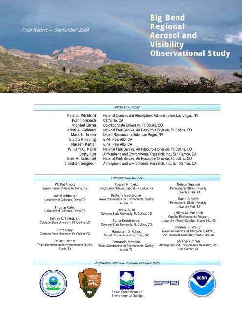
<strong>Final</strong> <strong>Report</strong> — September 2004<br />
Big Bend<br />
Regional<br />
Aerosol and<br />
Visibility<br />
Observational <strong>Study</strong><br />
PRIMARY AUTHORS<br />
Marc L. Pitchford<br />
Ivar Tombach<br />
Michael Barna<br />
Kristi A. Gebhart<br />
Mark C. Green<br />
Eladio Knipping<br />
Naresh Kumar<br />
William C. Malm<br />
Betty Pun<br />
Bret A. Schichtel<br />
Christian Seigneur<br />
National Oceanic and Atmospheric Administration, Las Vegas, NV<br />
Camarillo, CA<br />
Colorado State University, Ft. Collins, CO<br />
National Park Service, Air Resources Division, Ft. Collins, CO<br />
<strong>Desert</strong> <strong>Research</strong> <strong>Institute</strong>, Las Vegas, NV<br />
EPRI, Palo Alto, CA<br />
EPRI, Palo Alto, CA<br />
National Park Service, Air Resources Division, Ft. Collins, CO<br />
Atmospheric and Environmental <strong>Research</strong>, Inc., San Ramon, CA<br />
National Park Service, Air Resources Division, Ft. Collins, CO<br />
Atmospheric and Environmental <strong>Research</strong>, Inc., San Ramon, CA<br />
W. Pat Arnott<br />
<strong>Desert</strong> <strong>Research</strong> <strong>Institute</strong>, Reno, NV<br />
Lowell Ashbaugh<br />
University of California, Davis CA<br />
Thomas Cahill<br />
University of California, Davis CA<br />
Jeffrey L. Collett, Jr.<br />
Colorado State University, Ft. Collins, CO<br />
Derek Day<br />
Colorado State University, Ft. Collins, CO<br />
Stuart Dattner<br />
Texas Commission on Environmental Quality,<br />
Austin, TX<br />
CONTRIBUTING AUTHORS<br />
Russell N. Dietz<br />
Brookhaven National Laboratory, Upton, NY<br />
Bethany Georgoulias<br />
Texas Commission on Environmental Quality,<br />
Austin, TX<br />
Jenny Hand<br />
Colorado State University, Ft. Collins, CO<br />
Sonia Kreidenweis<br />
Colorado State University, Ft. Collins, CO<br />
Hampden D. Kuhns<br />
<strong>Desert</strong> <strong>Research</strong> <strong>Institute</strong>, Reno, NV<br />
Fernando Mercado<br />
Texas Commission on Environmental Quality,<br />
Austin, TX<br />
Nelson Seaman<br />
Pennsylvania State University,<br />
University Park, PA<br />
David Stauffer<br />
Pennsylvania State University,<br />
University Park, PA<br />
Jeffrey M. Vukovich<br />
Carolina Environmental Program,<br />
University of North Carolina, Chapel Hill, NC<br />
Thomas B. Watson<br />
National Oceanic and Atmospheric Admin.,<br />
Air Resources Laboratory, Idaho Falls, ID<br />
Shiang-Yuh Wu<br />
Atmospheric and Environmental <strong>Research</strong>, Inc.,<br />
San Ramon, CA<br />
SPONSORING AND CONTRIBUTING ORGANIZATIONS<br />
Texas Commission on<br />
Environmental Quality
Note to Readers<br />
This report relies extensively on color its charts and figures. Although the charts in the<br />
report are designed so that their meanings can generally be discerned from a black-and-white<br />
copy, full understanding of the information in some complex figures can only be achieved<br />
when they are viewed in color. Adobe Acrobat files containing the report and appendix are<br />
available on compact disc (CD) at the back of the original printed versions of the report and<br />
from the IMPROVE web site at http://vista.cira.colostate.edu/improve/.
<strong>Final</strong> <strong>Report</strong> — September 2004<br />
Preface<br />
The following is a report about the results of a study concerning the causes of<br />
visibility impairment at Big Bend National Park (NP) in west Texas. The study was<br />
prompted by observations in the early 1990s that visibility at the Park was frequently<br />
degraded and was apparently getting worse.<br />
A preliminary study was sponsored by the U.S. Environmental Protection Agency<br />
(EPA), the National Park Service (NPS), and governmental agencies from Mexico. This<br />
preliminary study was conducted in 1996 and a report of its findings released in January<br />
1999. The findings indicated that fine particulate sulfur compounds played a large role in<br />
observed impairment and that there was apparent transport of particulate sulfur compounds<br />
from sources in Mexico and the U.S. The preliminary report concluded that, in order to get a<br />
better understanding of the contributors to impairment at Big Bend NP, an enhanced study<br />
would be necessary that expanded the scope of the field measurement activities and<br />
expanded the spatial domain of the preliminary study, particularly to the northeast, south, and<br />
into the Gulf of Mexico.<br />
The EPA, the NPS, and the Texas Commission on Environmental Quality (TCEQ)<br />
comprised the Steering Committee for the enhanced study, the Big Bend Regional Aerosol<br />
and Visibility Observational (<strong>BRAVO</strong>) <strong>Study</strong>. In April 1999, Mexico elected not to<br />
participate in the <strong>Study</strong>, which resulted in the <strong>Study</strong> being unable to gather ambient<br />
monitoring and atmospheric tracer release data in Mexico. Although this was a disappointing<br />
development, the monitoring and atmospheric tracer protocols were altered to maximize data<br />
collection in the U.S. border area nearest Mexico. The <strong>BRAVO</strong> Technical Sub-committee<br />
designed and directed the field-measurement portion of this study that ran from July through<br />
October 1999, and interpretation and analyses of these field data were completed in early<br />
2004.<br />
The <strong>BRAVO</strong> <strong>Study</strong> was designed as an investigation of the causes of haze at Big<br />
Bend National Park, but not as an assessment of regulatory options. The <strong>Study</strong> constituted<br />
one of the largest and most comprehensive visibility field studies and air quality modeling<br />
evaluation efforts conducted in the U.S. It used state-of-the-science monitoring, air quality<br />
modeling, and laboratory and statistical analyses and involved over 30 researchers from<br />
research and academic institutions throughout the U.S. It used inert atmospheric tracers over<br />
a huge geographic scale and made use of the best available air emissions input data.<br />
Evaluation of the collected data continued for over three years after the end of the 1999 field<br />
study.<br />
While the Steering Committee was responsible for the ultimate publication of the<br />
<strong>BRAVO</strong> final report, the Steering Committee relied upon the <strong>BRAVO</strong> Technical Subcommittee<br />
to conduct or sponsor detailed analyses of the field data and source-region<br />
attribution analyses and to prepare the final report. Findings presented in the final report<br />
were thoroughly discussed by the Steering Committee, the Technical Sub-committee, and a<br />
i
<strong>Final</strong> <strong>Report</strong> — September 2004<br />
Non-governmental Sub-committee consisting of industry and environmental advocacy<br />
groups.<br />
The final report provides estimates of the contributions of broad geographic regions<br />
to visibility impairment at the Park during the study period. Contributions from the eastern<br />
U.S., eastern Texas, and Mexico were noted. Because of the relative proximity of the<br />
Carbón I and II power plants to the Park, contributions specific to those facilities were<br />
estimated in this analysis. Such source-specific calculations were not made for other sources<br />
in the study domain. Of particular significance was the indication that sources over a broad<br />
geographic region play roles in the observed visibility impairment in the Park, suggesting too<br />
that the solution should be based on international and regional, multi-State strategies.<br />
The confidence in these results notwithstanding, it must be emphasized that the<br />
endorsement of these findings by the <strong>BRAVO</strong> Steering Committee is made with the<br />
understanding that uncertainties exist and that analysis tools, no matter how sophisticated,<br />
only approximate atmospheric transport and chemical reactions. However, the Steering<br />
Committee is confident that the results of the study have been fairly presented with the<br />
concomitant caveats.<br />
The <strong>BRAVO</strong> Steering Committee wishes to acknowledge the commitment and<br />
contribution of all that participated in this study and the preparation of this report. Our<br />
understanding of the science of the effects of atmospheric aerosol on visibility has been<br />
greatly expanded, as has our understanding of the causes of visibility impairment at Big Bend<br />
NP.<br />
As the Steering Committee for the <strong>BRAVO</strong> <strong>Study</strong>:<br />
Mark A. Scruggs, Ph.D.<br />
National Park Service<br />
Herbert W. Williams<br />
Texas Commission on Environmental Quality<br />
James W. Yarbrough<br />
U.S. Environmental Protection Agency<br />
ii
<strong>Final</strong> <strong>Report</strong> — September 2004<br />
Acknowledgments<br />
The <strong>BRAVO</strong> <strong>Study</strong> could not have been accomplished without the enthusiastic<br />
support of participant organizations and individuals. From the initial planning in 1997,<br />
through the four-month ambient monitoring program in 1999, to the assessment process, and<br />
culminating in 2004 with the preparation of the final report, this study has been fortunate to<br />
include many talented and dedicated individuals from a number of organizations functioning<br />
together as a team. We are indebted to both the individuals for their thoughtful and energetic<br />
participation, and to their parent organizations that permitted and encouraged involvement by<br />
their staff.<br />
The list of organizations that participated in the <strong>BRAVO</strong> <strong>Study</strong> includes<br />
• Sponsors: U.S. Environmental Protection Agency, National Park Service, and the<br />
Texas Commission on Environmental Quality;<br />
• Contributors: EPRI, and the National Oceanic and Atmospheric Administration -<br />
Air Resources Laboratory;<br />
• <strong>Research</strong> Institutions and Universities: University of California - Davis, <strong>Desert</strong><br />
<strong>Research</strong> <strong>Institute</strong> and the Cooperative <strong>Institute</strong> for Atmospheric Science and<br />
Terrestrial Applications at the University of Nevada, Cooperative <strong>Institute</strong> for<br />
<strong>Research</strong> in the Atmosphere at Colorado State University, Pennsylvania State<br />
University, Carolina Environmental Program at the University of North Carolina,<br />
and Brookhaven National Laboratory;<br />
• Consulting Firms: Atmospheric and Environmental <strong>Research</strong>, Inc, Air Resource<br />
Specialists, Inc, and Aerosol Dynamics; and<br />
• Stakeholders: the Environmental Defense, the Sierra Club, American Electric<br />
Power, TXU, and Reliant Energy.<br />
The list below includes the individual participants that are not already acknowledged<br />
on the cover page as authors. It takes a lot of good people to accomplish a program of this<br />
magnitude and we were lucky to have a great team.<br />
• Ramon Alvarez ................Environmental Defense, Austin, TX<br />
• Thomas N. Braverman.....USEPA, <strong>Research</strong> Triangle Park, NC<br />
• Pete Breitenbach ..............Texas Commission on Environ. Quality, Austin, TX<br />
• Judith C. Chow.................<strong>Desert</strong> <strong>Research</strong> <strong>Institute</strong>, Reno, NV<br />
• N. N. Dharmarajan...........American Electric Power, Dallas, TX<br />
• Bright Dornblazer ............Texas Commission on Environ. Quality, Austin, TX<br />
• Robert C. Eldred ..............University of California, Davis, CA<br />
• Vic Etyemezian................<strong>Desert</strong> <strong>Research</strong> <strong>Institute</strong>, Las Vegas, NV<br />
• Miguel Flores...................USEPA Region VI, Dallas, TX<br />
iii
<strong>Final</strong> <strong>Report</strong> — September 2004<br />
Acknowledgments (continued)<br />
• Brian Foster......................Texas Commission on Environ. Quality, Austin, TX<br />
• Michael George................National Park Service, Austin, TX<br />
• Eric Gribbin .....................Texas Commission on Environ. Quality, Austin, TX<br />
• Mike Hannigan.................Colorado State University, Ft. Collins, CO<br />
• David Harper....................Texas Commission on Environ. Quality, Austin, TX<br />
• Susanne Hering ................Aerosol Dynamics, Berkeley, CA<br />
• Richard Karp....................Minerals Management Service, New Orleans, LA<br />
• John Kush.........................Reliant Energy, Houston, TX<br />
• Taeyoung Lee...................Colorado State University, Ft. Collins, CO<br />
• Chuck McDade ................University of California, Davis, CA<br />
• Jocelyn Mellberg..............Texas Commission on Environ. Quality, Austin, TX<br />
• Shannon Minto.................Texas Commission on Environ. Quality, Austin, TX<br />
• John Molenar ...................Air Resource Specialists, Ft. Collins, CO<br />
• Greg Newman ..................Reliant Energy, Houston, TX<br />
• Jill Riley...........................Colorado State University, Ft. Collins, CO<br />
• Dick Robertson ................TXU, Dallas, TX<br />
• Mark Scruggs...................National Park Service, Denver, CO<br />
• Eli Sherman......................Colorado State University, Ft. Collins, CO<br />
• Usha Turner .....................TXU, Dallas, TX<br />
• John Vimont.....................National Park Service, Denver, CO<br />
• John G. Watson................<strong>Desert</strong> <strong>Research</strong> <strong>Institute</strong>, Reno, NV<br />
• Herb Williams..................Texas Commission on Environ. Quality, Austin, TX<br />
• James W. Yarbrough........USEPA Region VI, Dallas, TX<br />
iv
<strong>Final</strong> <strong>Report</strong> — September 2004<br />
Table of Contents<br />
Page<br />
Preface........................................................................................................................................ i<br />
Acknowledgments.................................................................................................................... iii<br />
Table of Contents.......................................................................................................................v<br />
List of Figures.......................................................................................................................... xi<br />
List of Tables ...........................................................................................................................xx<br />
List of Abbreviations and Acronyms................................................................................... xxiv<br />
EXECUTIVE SUMMARY .................................................................................................ES-1<br />
1. TECHNICAL OVERVIEW ........................................................................................... 1-1<br />
Which are the major aerosol components contributing to haze at Big Bend NP<br />
throughout a year?............................................................................................ 1-2<br />
How does the composition of haze vary at Big Bend National Park throughout a<br />
year during the haziest days? ........................................................................... 1-4<br />
How does airflow to Big Bend National Park vary throughout the year?.................... 1-5<br />
Where are emission sources that may cause particulate sulfate compounds that<br />
contribute to Big Bend haze? ........................................................................... 1-7<br />
How does the composition of haze vary at Big Bend National Park during the<br />
four-month <strong>BRAVO</strong> <strong>Study</strong> period? ................................................................. 1-9<br />
How did different source regions contribute to particulate sulfate compounds<br />
affecting haze levels at Big Bend National Park during the <strong>BRAVO</strong><br />
<strong>Study</strong> period?.................................................................................................. 1-10<br />
How did different source regions contribute to haze levels at Big Bend National<br />
Park during the <strong>BRAVO</strong> <strong>Study</strong> period?......................................................... 1-14<br />
How applicable are the particulate sulfate attribution results for the <strong>BRAVO</strong><br />
<strong>Study</strong> period to other years or times of year?................................................. 1-16<br />
2. INTRODUCTION .......................................................................................................... 2-1<br />
2.1 Setting................................................................................................................. 2-1<br />
2.2 <strong>Study</strong> Goals......................................................................................................... 2-3<br />
2.3 Management ....................................................................................................... 2-3<br />
2.4 Preliminary <strong>Study</strong> ............................................................................................... 2-3<br />
2.5 Seasonality of the Aerosol Components of Light Extinction ............................. 2-5<br />
3. STUDY DESIGN AND IMPLEMENTATION............................................................. 3-1<br />
3.1 Selection of the <strong>Study</strong> Period ............................................................................. 3-1<br />
3.2 Use of Synthetic Tracers..................................................................................... 3-2<br />
3.2.1 Tracer Release ...................................................................................... 3-2<br />
3.2.2 Tracer Monitoring ................................................................................ 3-5<br />
3.3 Aerosol and Gaseous Measurements.................................................................. 3-6<br />
3.4 Optical Measurements ...................................................................................... 3-11<br />
v
<strong>Final</strong> <strong>Report</strong> — September 2004<br />
Table of Contents (continued)<br />
Page<br />
3.5 Meteorological Measurements.......................................................................... 3-11<br />
3.6 Source Characterization.................................................................................... 3-13<br />
3.7 Aircraft Measurements ..................................................................................... 3-14<br />
4. EMISSIONS INFORMATION ...................................................................................... 4-1<br />
4.1 Emission Inventory............................................................................................. 4-1<br />
4.2 Emissions Modeling ........................................................................................... 4-5<br />
4.3 Emissions Inventory Assessment ....................................................................... 4-7<br />
5. THE ATMOSPHERIC ENVIRONMENT OBSERVED AT BIG BEND<br />
NATIONAL PARK DURING THE <strong>BRAVO</strong> STUDY ................................................. 5-1<br />
5.1 Particulate Matter Characterization by the Routine Measurement Network...... 5-1<br />
5.1.1 Particulate Matter Temporal and Spatial Characteristics..................... 5-1<br />
5.1.2 Properties of Particulate Matter at Big Bend National Park ................ 5-4<br />
5.2 Detailed Characterization of the Particulate Matter at Big Bend National<br />
Park................................................................................................................... 5-6<br />
5.2.1 Ionic Composition of Big Bend Particulate Matter.............................. 5-7<br />
5.2.2 Short Time Resolution Sulfate Concentrations at Big Bend................ 5-8<br />
5.2.3 Organic Source Markers in Big Bend Aerosol................................... 5-10<br />
5.2.4 Particle Size Distribution ................................................................... 5-12<br />
5.2.5 Very Fine PM as a Source Tracer ...................................................... 5-13<br />
5.3 Characterization of Optical Conditions at Big Bend National Park ................. 5-15<br />
5.3.1 Light Absorption Measurements........................................................ 5-15<br />
5.3.2 Optical Measurements of the Big Bend Atmosphere......................... 5-19<br />
5.4 Meteorology During the <strong>BRAVO</strong> <strong>Study</strong> .......................................................... 5-21<br />
5.5 Perfluorocarbon Tracer Experiment Findings .................................................. 5-26<br />
5.5.1 Continuous Tracer Results ................................................................. 5-26<br />
5.5.2 Analysis of Timing Tracer Data......................................................... 5-30<br />
6. ANALYSIS OF <strong>BRAVO</strong> MEASUREMENTS.............................................................. 6-1<br />
6.1 Collocated Measurements................................................................................... 6-1<br />
6.2 Fine PM Mass Closure........................................................................................ 6-3<br />
6.3 Extinction Budget ............................................................................................... 6-4<br />
6.3.1 Light Scattering by Dry Particles ......................................................... 6-4<br />
6.3.2 Species Contributions to Light Extinction ........................................... 6-5<br />
6.4 Evaluation of the IMPROVE Equation for Estimating Light Extinction at<br />
Big Bend National Park.................................................................................... 6-8<br />
7. STUDY PERIOD REPRESENTATIVENESS .............................................................. 7-1<br />
7.1 Meteorology........................................................................................................ 7-1<br />
7.2 Transport Climatology........................................................................................ 7-4<br />
7.3 Aerosol and Light Extinction.............................................................................. 7-9<br />
7.4 Assessment of <strong>BRAVO</strong> <strong>Study</strong> Representativeness .......................................... 7-19<br />
vi
<strong>Final</strong> <strong>Report</strong> — September 2004<br />
Table of Contents (continued)<br />
Page<br />
8. ATTRIBUTION ANALYSIS AND MODELING METHODS .................................... 8-1<br />
8.1 Data Analysis Methods....................................................................................... 8-1<br />
8.1.1 Tracer Methods – TAGIT .................................................................... 8-1<br />
8.1.2 Empirical Orthogonal Function Analysis............................................. 8-3<br />
8.1.3 Factor Analysis..................................................................................... 8-4<br />
8.2 Meteorological Fields ......................................................................................... 8-4<br />
8.2.1 EDAS ................................................................................................... 8-5<br />
8.2.2 FNL ...................................................................................................... 8-5<br />
8.2.3 MM5..................................................................................................... 8-6<br />
8.3 Trajectory-Based Analyses................................................................................. 8-7<br />
8.3.1 ATAD Trajectories............................................................................... 8-7<br />
8.3.2 HYSPLIT Trajectories ......................................................................... 8-8<br />
8.3.3 CAPITA Monte Carlo Trajectories ...................................................... 8-8<br />
8.3.4 Ensemble Air-Mass History Analyses ................................................. 8-9<br />
8.3.5 Trajectory Mass Balance (TrMB) ........................................................ 8-9<br />
8.3.6 Forward Mass Balance Regression (FMBR) ..................................... 8-12<br />
8.4 Air Quality Simulation Modeling..................................................................... 8-14<br />
8.4.1 CAPITA Monte Carlo ........................................................................ 8-14<br />
8.4.2 REMSAD ........................................................................................... 8-15<br />
8.4.3 CMAQ................................................................................................ 8-16<br />
8.4.4 Synthesized REMSAD and CMAQ ................................................... 8-18<br />
8.5 Attribution Source Regions .............................................................................. 8-18<br />
8.6 Visualization of Spatial Patterns....................................................................... 8-21<br />
9. EVALUATION OF SOURCE ATTRIBUTION METHODS ....................................... 9-1<br />
9.1 Evaluation of Simulations of Meteorological Fields .......................................... 9-1<br />
9.1.1 Evaluation of MM5 Surface Meteorology Simulations ....................... 9-2<br />
9.1.2 Comparison of MM5, EDAS, and FNL Wind Fields to Radar<br />
Wind Profiler Measurements ............................................................... 9-5<br />
9.1.3 Evaluation of REMSAD/MM5 Simulations of Precipitation and<br />
Clouds................................................................................................... 9-9<br />
9.2 Sensitivity of Trajectories to Wind Fields........................................................ 9-13<br />
9.2.1 Effect of Wind Field Choice .............................................................. 9-14<br />
9.2.2 Effect of Trajectory Model Choice .................................................... 9-15<br />
9.2.3 Effect of Back Trajectory Start Height .............................................. 9-16<br />
9.2.4 Effect of Using FNL Winds in October ............................................. 9-17<br />
9.3 Evaluation of the Trajectory Mass Balance (TrMB) Method using<br />
Perfluorocarbon Tracer Measurements .......................................................... 9-17<br />
9.4 Evaluation of the CAPITA Monte Carlo Model Using Perfluorocarbon<br />
Tracer Measurements ..................................................................................... 9-20<br />
vii
<strong>Final</strong> <strong>Report</strong> — September 2004<br />
Table of Contents (continued)<br />
Page<br />
9.5 Evaluation of the Forward Mass Balance Regression (FMBR) Method<br />
Using Perfluorocarbon Tracer Measurements................................................ 9-25<br />
9.5.1 Retrieval of Tracer Release Locations and Rates............................... 9-25<br />
9.5.2 Source Apportionment of Tracer Concentrations .............................. 9-27<br />
9.5.3 Discussion of FMBR Tracer Evaluation ............................................ 9-28<br />
9.6 Evaluation of the Tracer Mass Balance (TrMB) Method Using<br />
REMSAD-Modeled Sulfate Concentrations .................................................. 9-28<br />
9.7 Evaluation of the Forward Mass Balance Regression (FMBR) Method<br />
Using REMSAD-Modeled Sulfate Concentrations........................................ 9-32<br />
9.8 Evaluation of REMSAD Simulations of Perfluorocarbon Tracers................... 9-34<br />
9.9 Evaluation of REMSAD Simulations of SO 2 , and Sulfate Measurements....... 9-39<br />
9.10 Evaluation of CMAQ Simulations of Perfluorocarbon Tracers ....................... 9-45<br />
9.11 Evaluation of CMAQ Simulations of SO 2 , Sulfate, and Other Aerosol<br />
Components.................................................................................................... 9-51<br />
9.11.1 Development of Base Case ................................................................ 9-51<br />
9.11.2 Base Case Performance...................................................................... 9-53<br />
9.11.3 Discussion of CMAQ-MADRID Performance .................................. 9-63<br />
9.12 Synthesis Inversion – Merging Modeled Source Apportionment Results<br />
and Receptor Data .......................................................................................... 9-64<br />
9.13 Conclusions Concerning Performance of the Source Attribution Methods ..... 9-66<br />
10. SOURCE ATTRIBUTIONS BY AMBIENT DATA ANALYSIS.............................. 10-1<br />
10.1 Sulfur Attributions via TAGIT ......................................................................... 10-1<br />
10.2 Attribution of PM 2.5 Components via Exploratory Factor Analysis................. 10-3<br />
10.3 Attribution of Big Bend Particulate Sulfur and Soil via EOF Analysis ........... 10-7<br />
10.4 Transport Patterns to Big Bend during Periods of High and Low Sulfur<br />
Concentrations.............................................................................................. 10-11<br />
10.5 Attribution of Big Bend Particulate Sulfur via Trajectory Mass Balance<br />
(TrMB) ......................................................................................................... 10-15<br />
10.6 Attribution of Big Bend Sulfate via Forward Mass Balance Regression<br />
(FMBR) ........................................................................................................ 10-18<br />
11. SOURCE ATTRIBUTIONS BY AIR QUALITY MODELING................................. 11-1<br />
11.1 Sulfate Attribution via REMSAD..................................................................... 11-1<br />
11.2 Sulfate Attribution via CMAQ-MADRID...................................................... 11-11<br />
11.3 Refined Sulfate Attribution using Synthesized Modeling Approaches.......... 11-17<br />
12. ATTRIBUTION RECONCILIATION, CONCEPTUAL MODEL, AND<br />
LESSONS LEARNED ................................................................................................. 12-1<br />
12.1 Introduction....................................................................................................... 12-1<br />
12.2 Phase I: Tracer Screening and Evaluation........................................................ 12-3<br />
12.3 Phase II: Initial Application.............................................................................. 12-5<br />
12.4 Refined Attribution Approaches....................................................................... 12-8<br />
viii
<strong>Final</strong> <strong>Report</strong> — September 2004<br />
Table of Contents (continued)<br />
Page<br />
12.5 Haze Source Attribution ................................................................................. 12-12<br />
12.6 Big Bend Haze Conceptual Model ................................................................. 12-15<br />
12.7 Lessons Learned and Recommendations........................................................ 12-19<br />
12.7.1 Overall Design and Management..................................................... 12-20<br />
12.7.2 Field Measurements ......................................................................... 12-21<br />
12.7.3 Source Attribution Approaches........................................................ 12-22<br />
12.7.4 Results .............................................................................................. 12-24<br />
13. REFERENCES............................................................................................................. 13-1<br />
APPENDIX.......................................................... CD-ROM disc on the last page of this report<br />
A.1 Baylor University (2000). 1999 Executive Summary: Airborne Pollution<br />
Monitoring Services. ................filename: A1_Baylor2000AircraftMeasurements.pdf<br />
A.2 Cahill, T.A., et al. (2003). UC Davis DELTA Group <strong>Final</strong> report to<br />
<strong>BRAVO</strong> on the project – Very fine (0.26 > Dp > 0.09 µm) Silicon plus<br />
Sulfur as a Tracer of Coal Fired Power Plants during <strong>BRAVO</strong>.<br />
....................................................... filename: A2_Cahill2003UCDavisSiliconSulfur.pdf<br />
A.3 Georgoulias, B. (2003). Was <strong>BRAVO</strong> Meteorology “Typical”?<br />
..........................................................filename: A3_Georgoulias2003Meteorology.pdf<br />
A.4 Georgoulias, B., et al. (2003). Evaluation of the Reconstruction Equation<br />
at Big Bend during <strong>BRAVO</strong> & Using Factor Analysis to Relate Aerosol<br />
Concentrations to Light Extinction.<br />
........................................................... filename: A4_Georgoulias2003ReconEqFA.pdf<br />
A.5 Kuhns, H., et al. (2003). Big Bend Regional Aerosol and Visibility<br />
Observational (<strong>BRAVO</strong>) <strong>Study</strong> Emissions Inventory.<br />
.......................................................................filename: A5_Kuhns2003EmissInv.pdf<br />
A.6 Mercado, F., et al. (2004). Application of Factor Analysis to the <strong>BRAVO</strong><br />
Dataset. .............................................filename: A6_Mercado2004FactorAnalysis.pdf<br />
A.7 Pun et al. (2004). Modeling Analysis of the Big Bend Regional Aerosol<br />
Visibility Observational (Bravo) <strong>Study</strong>.<br />
.......................................................................... filename: A7_Pun2004Modeling.pdf<br />
A.8 Schichtel et al. (2004). Big Bend Regional Aerosol and Visibility<br />
Observational (<strong>BRAVO</strong>) <strong>Study</strong> Results: Air Quality Data and Source<br />
Attribution Analyses Results from the National Park Service /<br />
Cooperative <strong>Institute</strong> for <strong>Research</strong> in the Atmosphere.<br />
............................................................... filename: A8_Schichtel2004CIRA<strong>Report</strong>.pdf<br />
A.8.1 REMSAD Animations<br />
.................................................... filenames: A8_so2_oct1999.avi<br />
...................................................................................... A8_so4_oct1999.avi<br />
...........................................................................A8_so4_clouds_oct1999.avi<br />
........................................................................A8_winds_clouds_oct1999.avi<br />
ix
<strong>Final</strong> <strong>Report</strong> — September 2004<br />
Table of Contents (continued)<br />
A.8.2<br />
A.8.3<br />
Page<br />
Backward Trajectories<br />
................................. filenames: A8_Appendix4b_CAPITAMC_Trajectories.ppt<br />
......................................................A8_Appendix4c_HYSPLIT_Trajectories.ppt<br />
..........................................................A8_Appendix4d_ATAD_Trajectories.ppt<br />
Daily Maps of Fine Particulate Sulfur Concentrations<br />
......................................... filename: A8_Appendix8b_DailySulfurPatterns.ppt<br />
A.9 Seaman, N.L.; and Stauffer, D.R. (2003). <strong>Final</strong> <strong>Report</strong> to Electric Power<br />
<strong>Research</strong> <strong>Institute</strong> Contract EP-P3883/C1886 for MM5 Modeling in<br />
support of the Big Bend Regional Aerosol and Visibility Observation<br />
<strong>Study</strong> (<strong>BRAVO</strong>). ............................... filename: A9_Seaman2003MM5Modeling.pdf<br />
A.10 Vukovich, J. (2002). Technical <strong>Report</strong>: Emissions Processing for the Big<br />
Bend Regional Aerosol and Visibility Observational (<strong>BRAVO</strong>) <strong>Study</strong>.<br />
...........................................................filename: A10_Vukovich2002EmissProcess.pdf<br />
A.11 Watson, T.B., et al. (2000). The Perfluorocarbon Tracer Releases during<br />
the Big Bend Regional Aerosol and Visibility Observational (<strong>BRAVO</strong>)<br />
<strong>Study</strong>. ...........................................................filename: A11_Watson2000Tracer.pdf<br />
Pitchford, M.L., et al. (2004). Big Bend Regional Aerosol and Visibility<br />
Observational <strong>Study</strong> <strong>Final</strong> <strong>Report</strong>. ............... filename: <strong>BRAVO</strong><strong>Final</strong><strong>Report</strong>9-04.pdf<br />
x
<strong>Final</strong> <strong>Report</strong> — September 2004<br />
List of Figures<br />
Page<br />
Figure 1-1<br />
Figure 1-2<br />
Figure 1-3<br />
Figure 1-4<br />
Figure 1-5<br />
Figure 1-6<br />
Figure 1-7<br />
Figure 1-8<br />
Figure 1-9<br />
Figure 1-10<br />
Figure 1-11<br />
Big Bend National Park five-year composite contributions to haze by<br />
components. .............................................................................................................1-3<br />
Quarterly aerosol contributions to light extinction averaged over five years<br />
(1998 – 2002). .........................................................................................................1-4<br />
Examples of geographic distribution of the fraction of time that air parcels<br />
spend during the five days prior to arriving at Big Bend National Park for the<br />
months of January, May, July and September based upon a five-year analysis<br />
period (1998 to 2002). .............................................................................................1-6<br />
Monthly fractions of time that air parcels spend in a region prior to arrival at<br />
Big Bend, based on five-day back trajectory calculations for the five-year<br />
period from 1998 to 2002. .......................................................................................1-6<br />
(Left) SO 2 emissions based on the 1999 <strong>BRAVO</strong> emissions inventory used in<br />
the REMSAD and CMAQ-MADRID modeling. ....................................................1-8<br />
Contributions to haze by components during the <strong>BRAVO</strong> <strong>Study</strong> period.<br />
(LAC is light absorbing carbon.)...............................................................................1-9<br />
Estimates by several data analysis and modeling methods of the study-period<br />
averaged percent contributions to particulate sulfate at Big Bend by U.S. and<br />
Mexico sources. .....................................................................................................1-12<br />
Smoothed daily estimates by source regions to particulate sulfate<br />
concentration (top plot) and fraction of total predicted particulate sulfate<br />
(bottom plot) at Big Bend during the study period. ...............................................1-13<br />
Estimated contributions to light extinction by various particulate sulfate<br />
source regions. .......................................................................................................1-15<br />
Estimated contributions by particulate sulfate source regions to Big Bend<br />
light extinction levels for the 1/5 haziest days and the 1/5 least hazy days of<br />
the <strong>BRAVO</strong> <strong>Study</strong> period. ........................................................................................15<br />
Fraction of time that air parcels spent during five-day trajectories for periods<br />
with the 20% highest concentrations of particulate sulfate compounds and for<br />
the periods with the 20% lowest concentrations of particulate sulfate<br />
compounds during the <strong>BRAVO</strong> <strong>Study</strong> period July through October 1999. ..........1-17<br />
Figure 2-1 Location map of Big Bend National Park in southwestern Texas. ..........................2-1<br />
Figure 2-2<br />
Texas and Mexico (above) and the terrain surrounding Big Bend National<br />
Park in western Texas and northern Mexico (below). .............................................2-2<br />
Figure 2-3 Map showing monitoring sites for preliminary visibility study. .............................2-4<br />
Figure 2-4<br />
Big Bend National Park five-year composite contributions to haze by<br />
components. .............................................................................................................2-5<br />
Figure 2-5 Big Bend extinction budget time plots of individual years. ....................................2-6<br />
xi
<strong>Final</strong> <strong>Report</strong> — September 2004<br />
List of Figures (continued)<br />
Page<br />
Figure 3-1<br />
Data recovery of 24-hr tracer sample data during the two periods when 24-hr<br />
tracer sampling took place. ......................................................................................3-7<br />
Figure 3-2 Network of 24-hour gas and aerosol sampling locations. .......................................3-9<br />
Figure 3-3 Network of 6-hour gas and aerosol sampling locations. .........................................3-9<br />
Figure 3-4 Upper-air meteorological sites. .............................................................................3-12<br />
Figure 4-1<br />
Figure 4-2<br />
Figure 4-3<br />
Figure 4-4<br />
Figure 5-1<br />
The <strong>BRAVO</strong> <strong>Study</strong> emission inventory was compiled for the shaded areas of<br />
the U.S. and Mexico shown here. ............................................................................4-2<br />
Locations of offshore platforms included in the <strong>BRAVO</strong> <strong>Study</strong> emissions<br />
inventory. .................................................................................................................4-4<br />
SO 2 emissions rates from the <strong>BRAVO</strong> <strong>Study</strong> emissions inventory are shown<br />
as proportional to the bar heights on the map. .........................................................4-4<br />
(Left) SO 2 emissions based on the 1999 <strong>BRAVO</strong> emissions inventory used in<br />
the REMSAD and CMAQ-MADRID modeling. ....................................................4-9<br />
Groups of <strong>BRAVO</strong> sampling sites that showed similar particulate matter<br />
behavior. ..................................................................................................................5-2<br />
Figure 5-2 Sulfate and SO 2 time series at K-Bar. .....................................................................5-2<br />
Figure 5-3 Composition of PM 2.5 aerosol throughout Texas during the August 29-<br />
September 4, 1999, sulfate episode at Big Bend. ....................................................5-3<br />
Figure 5-4<br />
Figure 5-5<br />
Figure 5-6<br />
Figure 5-7<br />
Figure 5-8<br />
Figure 5-9<br />
Timelines of the PM 2.5 molar ratio of NH 4 + /SO 4 2– and aerosol acidity at Big<br />
Bend National Park. ................................................................................................5-8<br />
Example of hourly fine sulfate and sulfur dioxide concentration<br />
measurements at Big Bend National Park. ..............................................................5-9<br />
Example of light scattering coefficient measured at ambient humidity for<br />
particles below 2.5 µm, compared with measured hourly-averaged sulfate<br />
concentration, accumulation mode volume and light scattering coefficient,<br />
and coarse mode particle scattering, all derived from physical size<br />
distribution measurements. ....................................................................................5-10<br />
The n-alkane carbon preference index (CPI) for the <strong>BRAVO</strong> organic aerosol<br />
sample composites. ................................................................................................5-11<br />
Timelines of dry particulate matter volume concentrations (in µm 3 /cm 3 ) at<br />
Big Bend National Park for the accumulation and coarse modes, as computed<br />
from measured size distributions. ..........................................................................5-13<br />
Timeline of very fine (0.26 µm > D p > 0.09 µm) silicon (x 25) and sulfur<br />
concentrations at Big Bend National Park during August 1999. ...........................5-14<br />
xii
<strong>Final</strong> <strong>Report</strong> — September 2004<br />
List of Figures (continued)<br />
Page<br />
Figure 5-10<br />
Figure 5-11<br />
Figure 5-12<br />
Figure 5-13<br />
Figure 5-14<br />
Comparisons of 12-hour averages of the photoacoustic light absorption<br />
measurements and the aethalometer black carbon measurements (top) and<br />
IMPROVE EC measurements (bottom) during the <strong>BRAVO</strong> <strong>Study</strong>. .....................5-17<br />
Comparison of hourly averaged black carbon and light absorption<br />
measurements during the <strong>BRAVO</strong> study time period of Figure 5-10. ..................5-18<br />
Average distribution of the measured components of extinction at Big Bend<br />
during the <strong>BRAVO</strong> <strong>Study</strong> period ............................................................................5-21<br />
Frequencies of wind directions at three height ranges during July-October<br />
1999, as measured by the <strong>BRAVO</strong> radar wind profilers. ......................................5-22<br />
July 1999 monthly resultant winds at 850 mb (approximately1500 m MSL),<br />
showing flow from the south in the Big Bend area. ..............................................5-23<br />
Figure 5-15 Surface weather map for 6 am CST on August 20, 1999. .....................................5-24<br />
Figure 5-16 Surface weather map for 6 am CST on August 29, 1999. .....................................5-24<br />
Figure 5-17 Surface weather map for 6 pm CST on September 11, 1999. ...............................5-25<br />
Figure 5-18 Surface weather map for 6 pm CST on September 13, 1999. ...............................5-26<br />
Figure 5-19<br />
Figure 5-20<br />
Figure 5-21<br />
Figure 5-22<br />
Figure 5-23<br />
Figure 5-24<br />
Figure 5-25<br />
Figure 5-26<br />
Time series of influence functions at 6-hr sampling sites for the Eagle Pass<br />
continuous tracer, ocPDCH. ..................................................................................5-28<br />
Time series of influence functions at 6-hr sampling sites for the Northeast<br />
Texas tracer, i-PPCH. ............................................................................................5-28<br />
Time series of influence functions at 6-hr sampling sites for the San Antonio<br />
tracer, PDCB. ........................................................................................................5-29<br />
Time series of influence functions at 6-hr sampling sites for the Houston<br />
tracer, PTCH. .........................................................................................................5-29<br />
Alternate day tracer PDCB versus continuous tracer ocPDCH influence<br />
functions at 6 hour sites for periods of timing tracer release (7/5/99- 9/13/99).<br />
.................................................................................................................................5-30<br />
Daytime only (8 am to 8 pm CDT) tracer PTCH versus continuous tracer<br />
ocPDCH influence functions at 6 hour sites for periods of timing tracer<br />
release (7/5/99- 9/13/99). ......................................................................................5-31<br />
Normalized ratio of PDCB to ocPDCH released from Eagle Pass at four<br />
monitoring sites. ....................................................................................................5-32<br />
Distribution of estimated transport times of Eagle Pass tracers to 6-hour<br />
monitoring sites in each 6-hour period during the timing tracer study (7/5/99-<br />
9/13/99). ................................................................................................................5-33<br />
xiii
<strong>Final</strong> <strong>Report</strong> — September 2004<br />
List of Figures (continued)<br />
Page<br />
Figure 6-1<br />
Figure 6-2<br />
Figure 6-3<br />
Figure 6-4<br />
Figure 6-5<br />
Figure 6-6<br />
Comparison of sulfate and ammonium measurements by UC Davis and<br />
Colorado State University. ......................................................................................6-1<br />
Molar ratio of ammonium to sulfate as measured by UC Davis and Colorado<br />
State University during the <strong>BRAVO</strong> <strong>Study</strong> period. ................................................6-2<br />
Nitrate concentrations at K-Bar as measured by UC Davis and Colorado<br />
State University during the <strong>BRAVO</strong> <strong>Study</strong> Period. ................................................6-3<br />
Calculated contributions to haze by components of the aerosol during the<br />
<strong>BRAVO</strong> <strong>Study</strong> period. ............................................................................................6-8<br />
Comparison of extinction measured by the BIBE1 transmissometer and<br />
calculated from PM species concentrations. .........................................................6-10<br />
Comparison of extinction measured by the BBEP transmissometer (with<br />
additional lamp brightening adjustments) with that calculated from PM<br />
species concentrations. ..........................................................................................6-13<br />
Figure 7-1 Comparison of wind roses for July 1995-1998 (left) and 1999 (right). ..................7-2<br />
Figure 7-2 Comparison of wind roses for August 1995-1998 (left) and 1999 (right). ..............7-3<br />
Figure 7-3 Comparison of wind roses for September 1995-1998 (left) and 1999 (right). ........7-3<br />
Figure 7-4 Comparison of wind roses for October 1995-1998 (left) and 1999 (right). ............7-4<br />
Figure 7-5<br />
Figure 7-6<br />
Figure 7-7<br />
Residence times for July-October 1999 (left) and the five-year July-October<br />
average (right), for 10 and 1,500 meter back-trajectory starting heights at Big<br />
Bend. .......................................................................................................................7-6<br />
Differences in residence times between July-October 1999 and the five-year<br />
(1998-2002) July-October average for all three back trajectory starting<br />
elevations. ................................................................................................................7-7<br />
Differences in residence times between July-October 1998, 2000, 2001, and<br />
2002 and the five-year (1998-2002) July-October average for the 500m<br />
starting elevation. ....................................................................................................7-8<br />
Figure 7-8 Big Bend extinction budget time plots of individual years. ..................................7-10<br />
Figure 7-9<br />
Figure 7-10<br />
Figure 7-11<br />
Big Bend National Park five-year composite contributions to haze by<br />
components. ...........................................................................................................7-11<br />
Means and standard deviations of concentrations of components of PM 10 at<br />
Big Bend National Park during four different averaging periods. ........................7-12<br />
Means and standard deviations of particle-caused light extinction estimated<br />
from concentrations of components of PM 10 at Big Bend National Park<br />
during four different averaging periods. ................................................................7-14<br />
xiv
<strong>Final</strong> <strong>Report</strong> — September 2004<br />
List of Figures (continued)<br />
Page<br />
Figure 7-12<br />
Figure 7-13<br />
Figure 7-14<br />
Figure 7-15<br />
Figure 7-16<br />
Estimated relative contributions of various particulate matter components to<br />
particle-caused light extinction during four different averaging periods. .............7-15<br />
Box plots of measured fine mass concentration frequency distributions<br />
during four different averaging periods. ................................................................7-15<br />
Box plots of measured coarse mass concentration frequency distributions<br />
during four different averaging periods. ................................................................7-16<br />
Box plots of ammonium sulfate concentration frequency distributions during<br />
four different averaging periods. ...........................................................................7-17<br />
Box plots of particle chemical extinction frequency distributions during four<br />
different averaging periods. ...................................................................................7-18<br />
Figure 8-1 Locations of the triply-nested MM5 domains, with grid resolutions of 36, 12,<br />
and 4 km. .................................................................................................................8-7<br />
Figure 8-2<br />
Figure 8-3<br />
Source areas with map identification numbers used for Trajectory Mass<br />
Balance Modeling. ................................................................................................8-11<br />
Locations of 17 source areas composed of 100-km grid virtual sources used<br />
to track transport and dispersion in the Forward Mass Balance Regression<br />
method. ..................................................................................................................8-13<br />
Figure 8-4 Map of the REMSAD attribution source regions. .................................................8-19<br />
Figure 8-5 The CMAQ-MADRID attribution source regions. ...............................................8-20<br />
Figure 8-6<br />
Figure 8-7<br />
Figure 8-8<br />
Figure 9-1<br />
Figure 9-2<br />
Figure 9-3<br />
Figure 9-4<br />
Plumes of a conservative tracer, released from four sites within Texas, as<br />
simulated by the REMSAD air quality model (4 October 1999). .........................8-21<br />
Comparison of spatial patterns of observed sulfate (left) and simulated<br />
sulfate (right) (19 August 1999). ...........................................................................8-22<br />
Precipitating clouds (yellow), non-precipitating clouds (blue), wind vectors,<br />
and streamlines predicted by the MM5 weather model (1 October 1999). ...........8-22<br />
Comparisons of MM5 and EDAS wind direction frequencies versus radar<br />
wind profiler measurements, by level above ground, for July-September 1999<br />
at Big Bend National Park. ......................................................................................9-8<br />
Comparisons of MM5 and EDAS wind direction frequencies versus radar<br />
wind profiler measurements, by level above ground, for July-September 1999<br />
at Llano, Texas. .....................................................................................................9-10<br />
Examples of REMSAD precipitation prediction and observed precipitation<br />
maps (for July 2, 1999). .........................................................................................9-11<br />
Examples of REMSAD predicted cloud cover and corresponding GOES<br />
satellite picture (for July 3, 1999). ........................................................................9-12<br />
xv
<strong>Final</strong> <strong>Report</strong> — September 2004<br />
List of Figures (continued)<br />
Page<br />
Figure 9-5<br />
Figure 9-6<br />
Examples of the effects of EDAS and MM5 wind fields on back trajectories<br />
produced by the CAPITA Monte Carlo model. .....................................................9-15<br />
Examples of the effect of start height on the trajectories produced by the<br />
HYSPLIT model with the EDAS wind field. ........................................................9-16<br />
Figure 9-7 The tracer release regions (shaded boxes) defined for the TrMB evaluation. .......9-18<br />
Figure 9-8<br />
Figure 9-9<br />
Figure 9-10<br />
Figure 9-11<br />
Figure 9-12<br />
Figure 9-13<br />
Figure 9-14<br />
Figure 9-15<br />
Figure 9-16<br />
Figure 9-17<br />
Figure 9-18<br />
Figure 9-19<br />
Comparison of observed and modeled tracer concentrations, for the Eagle<br />
Pass, San Antonio, and Houston tracers, at Big Bend National Park over the<br />
duration of the study. .............................................................................................9-22<br />
Comparison of spatially-averaged observed and modeled tracer<br />
concentrations in southwest Texas (in the same format as Figure 9-8). ................9-23<br />
FMBR reconstructions of the Eagle Pass and northeast Texas tracer release<br />
locations and rates. ................................................................................................9-26<br />
Average percentage source contributions to measured tracer at Big Bend, as<br />
estimated by FMBR (red) and as measured (blue). ...............................................9-28<br />
Scatter plots of REMSAD sulfate concentration attributions vs. number of<br />
endpoints for each of four large source areas using 5-day back trajectories<br />
from the CAPITA MC Model and MM5 winds. ...................................................9-31<br />
Example of the REMSAD-simulated dispersion of the four tracer plumes on<br />
28 September 1999. ...............................................................................................9-35<br />
Comparison of 24-hr three-site average REMSAD predictions (red) of the<br />
spatially-averaged concentrations in Big Bend National Park versus three-site<br />
average measurements (blue) for the continuous Eagle Pass tracer. .....................9-36<br />
Comparison of 24-hr three-site average REMSAD predictions (red) of the<br />
spatially-averaged concentrations in Big Bend National Park versus three-site<br />
average measurements (blue) for the northeast Texas tracer. ...............................9-37<br />
Comparison of 24-hr three-site average REMSAD predictions (red) of the<br />
spatially-averaged concentrations in Big Bend National Park versus three-site<br />
average measurements (blue) for the San Antonio tracer. .....................................9-37<br />
Comparison of 24-hr three-site average REMSAD predictions (red) of the<br />
spatially-averaged concentrations in Big Bend National Park versus three-site<br />
average measurements (blue) for the Houston tracer. ...........................................9-38<br />
Comparisons of observed (blue) and modeled (red) time series of 24-hr<br />
averaged concentrations of SO 2 , sulfate, and total sulfur at the K-Bar<br />
sampling site in Big Bend National Park. .............................................................9-39<br />
Smoothed REMSAD simulation of ground-level sulfate concentrations at<br />
1700 CDT on 28 September 1999. ........................................................................9-43<br />
xvi
<strong>Final</strong> <strong>Report</strong> — September 2004<br />
List of Figures (continued)<br />
Page<br />
Figure 9-20<br />
Figure 9-21<br />
Figure 9-22<br />
Figure 9-23<br />
Figure 9-24<br />
Figure 9-25<br />
Figure 9-26<br />
Figure 9-27<br />
Figure 9-28<br />
Scatter plots of REMSAD 24-hr sulfur concentration predictions versus<br />
measured values at 37 <strong>BRAVO</strong> network locations over the full <strong>BRAVO</strong><br />
<strong>Study</strong> period. .........................................................................................................9-45<br />
Measured (top) and CMAQ-simulated (bottom) time series of NE Texas<br />
tracer concentrations (in ppq) at K-Bar. ................................................................9-46<br />
Measured (top) and CMAQ-simulated (bottom) time series of Eagle Pass<br />
PDCH tracer concentrations (in ppq) at K-Bar. ....................................................9-47<br />
Measured (top) and CMAQ-simulated (bottom) time series of Houston tracer<br />
concentrations (in ppq) at K-Bar. ..........................................................................9-47<br />
Measured (top) and CMAQ-simulated (bottom) time series of San Antonio<br />
tracer concentrations (in ppq) at K-Bar. ................................................................9-48<br />
Spatial distributions of mean normalized bias and mean normalized error in<br />
CMAQ-MADRID predictions of fine sulfate over the <strong>BRAVO</strong> network. ............9-55<br />
Measured and simulated 24-hr SO 2 (top) and sulfate (bottom) concentrations<br />
at K-Bar. ................................................................................................................9-58<br />
Measured and simulated daily SO 2 concentrations (top) and fine sulfate<br />
concentrations (bottom) at Big Thicket. ................................................................9-59<br />
Compositions of observed and simulated PM 2.5 at K-Bar, averaged over the<br />
duration of the <strong>BRAVO</strong> <strong>Study</strong>. .............................................................................9-62<br />
Figure 10-1 Contour plot of locations of top 50 loadings scores for Factor 1 (Soils). ..............10-4<br />
Figure 10-2<br />
Figure 10-3<br />
Contour plot of locations of top 50 loadings scores for Factor 2 (Coal<br />
Burning). ...............................................................................................................10-4<br />
Contour plot of locations of top 50 loadings for Factor 3 (Undetermined<br />
source type). ..........................................................................................................10-5<br />
Figure 10-4 Contour plot of locations of top 50 loadings for Factor 4 (Smelting). ..................10-5<br />
Figure 10-5<br />
Figure 10-6<br />
Figure 10-7<br />
Figure 10-8<br />
Distribution of mean particulate sulfur concentrations over the portion of the<br />
study period when all sites had sufficiently complete data for EOF analysis. ......10-8<br />
Composite of mean sulfur concentrations (ng/m 3 ) measured during<br />
September and October in 1996 (the preliminary study) and 1999 (the<br />
<strong>BRAVO</strong> <strong>Study</strong>). ....................................................................................................10-9<br />
The four EOF analysis-derived spatial factors for particulate sulfur and their<br />
temporal weights during most of the <strong>BRAVO</strong> <strong>Study</strong> period. ..............................10-10<br />
Air mass transport patterns to Big Bend during three particulate sulfur<br />
episodes. ..............................................................................................................10-12<br />
xvii
<strong>Final</strong> <strong>Report</strong> — September 2004<br />
List of Figures (continued)<br />
Page<br />
Figure 10-9<br />
Figure 10-10<br />
Figure 10-11<br />
Figure 11-1<br />
Residence time probability distributions showing transport pathways during<br />
high particulate sulfur days, based on the EDAS/FNL wind fields. .....................10-13<br />
Residence time probability distributions showing transport pathways during<br />
high particulate sulfur days, based on the <strong>BRAVO</strong> 36km MM5 wind fields. ....10-14<br />
Residence time probability distributions showing transport pathways during<br />
low particulate sulfur days, based on the EDAS/FNL wind fields. .....................10-15<br />
Map of the REMSAD modeling domain and the four principal geographic<br />
regions to which sulfate at Big Bend National Park (red diamond) was<br />
attributed. ...............................................................................................................11-2<br />
Figure 11-2 REMSAD simulation of sulfate concentrations on 17 August 1999 at 1500<br />
UTC using the full <strong>BRAVO</strong> emissions inventory. ................................................11-3<br />
Figure 11-3<br />
Figure 11-4<br />
Figure 11-5<br />
Figure 11-6<br />
Figure 11-7<br />
Figure 11-8<br />
Figure 11-9<br />
Figure 11-10<br />
Figure 11-11<br />
REMSAD simulation of sulfate concentrations from emissions in the Eastern<br />
U.S. source region on 17 August 1999 at 1500 UTC. ...........................................11-4<br />
REMSAD simulation of sulfate concentrations from emissions in the<br />
Mexican source region on 17 August 1999 at 1500 UTC. ....................................11-4<br />
REMSAD simulation of sulfate concentrations from emissions in Texas on<br />
17 August 1999 at 1500 UTC. ...............................................................................11-5<br />
REMSAD simulation of sulfate concentrations from emissions in the<br />
Western U.S. source region on 17 August 1999 at 1500 UTC. .............................11-5<br />
REMSAD simulation of sulfate concentrations attributable to sulfur<br />
concentrations defined along the modeling domain boundaries by the<br />
GOCART global model on 17 August 1999 at 1500 UTC. ..................................11-6<br />
Observed and REMSAD-estimated sulfate concentrations at Big Bend and<br />
REMSAD-estimated contributions by source region (using the “emissions<br />
out” approach) for (a) the 4-month <strong>BRAVO</strong> <strong>Study</strong> period and (b-e) July<br />
through October, respectively. ..............................................................................11-7<br />
REMSAD-estimated relative attributions, of average sulfate concentrations at<br />
Big Bend for each source region (using the “emissions out” approach) for (a)<br />
the 4-month <strong>BRAVO</strong> <strong>Study</strong> period and (b-e) the months of July through<br />
October, respectively. ............................................................................................11-8<br />
Daily REMSAD attributions of sulfate concentrations at Big Bend to the four<br />
source regions and the GOCART boundary concentrations, based on the<br />
“emissions out” approach. .....................................................................................11-9<br />
Source regions used for CMAQ-MADRID sulfate attributions. No source<br />
attribution simulations were conducted for the open water Gulf of Mexico<br />
(red) region. .........................................................................................................11-12<br />
xviii
<strong>Final</strong> <strong>Report</strong> — September 2004<br />
List of Figures (continued)<br />
Page<br />
Figure 11-12<br />
Figure 11-13<br />
Figure 11-14<br />
Figure 11-15<br />
Figure 11-16<br />
CMAQ-MADRID average attribution of fine sulfate at K-Bar over the<br />
4-month <strong>BRAVO</strong> <strong>Study</strong> period, expressed as ratios of estimated average<br />
regionally-attributed concentrations of sulfate to average total estimated<br />
sulfate. .................................................................................................................11-13<br />
Daily CMAQ-MADRID attributions of sulfate concentrations (in µg/m 3 ) at<br />
Big Bend to the four source regions and the boundary concentrations. ..............11-15<br />
<strong>Study</strong>-period source attributions of fine sulfate (in µg/m 3 ) at K-Bar by the<br />
synthesized and original models. .........................................................................11-19<br />
Synthesized REMSAD estimates of K-Bar sulfate source attributions for<br />
seven selected episodes. ......................................................................................11-20<br />
Synthesized CMAQ-MADRID estimates of K-Bar sulfate source attributions<br />
for seven selected episodes. .................................................................................11-21<br />
Figure 11-17 Smoothed daily Synthesized CMAQ-MADRID attributions of sulfate at K-<br />
Bar. ......................................................................................................................11-22<br />
Figure 12-1<br />
Figure 12-2<br />
Figure 12-3<br />
Figure 12-4<br />
Figure 12-5<br />
Simulated surface layer PTCH tracer concentrations (released from Houston<br />
TX) for October 12 th 1999 generated by REMSAD at 36km and 12km and by<br />
CMAQ at 12km. ....................................................................................................12-4<br />
Smoothed daily <strong>BRAVO</strong> Estimates of contributions to Big Bend particulate<br />
sulfate by source region. ......................................................................................12-12<br />
Estimated contributions to light extinction by various particulate sulfate<br />
source regions. .....................................................................................................12-13<br />
<strong>BRAVO</strong> Estimates of contributions by particulate sulfate source regions to<br />
Big Bend light extinction levels for the 1/5 haziest days and the 1/5 least<br />
hazy days of the <strong>BRAVO</strong> <strong>Study</strong> period. .............................................................12-14<br />
Big Bend National Park five-year composite contributions to haze by<br />
components. .........................................................................................................12-15<br />
Figure 12-6 Big Bend extinction budget time plots for individual years. ...............................12-16<br />
Figure 12-7<br />
Figure 12-8<br />
Monthly fractions of time that air parcels spend in a region prior to arrival at<br />
Big Bend in 1998 to 2002 are shown as solid bars, based on five-day back<br />
trajectory calculations. .........................................................................................12-17<br />
Percent of time that air parcels en route to Big Bend spent over various<br />
locations during five-day trajectories for periods with the 20% highest<br />
concentrations of particulate sulfate compounds at Big Bend (left) and for the<br />
periods with the 20% lowest concentrations of particulate sulfate compounds<br />
at Big Bend (right) during the <strong>BRAVO</strong> <strong>Study</strong> period of July through October<br />
1999. ....................................................................................................................12-19<br />
xix
<strong>Final</strong> <strong>Report</strong> — September 2004<br />
List of Tables<br />
Table 3-1 Tracer release schedule first phase of study. ...........................................................3-4<br />
Table 3-2 Tracer release schedule for the second half of the study. ........................................3-4<br />
Page<br />
Table 3-3<br />
PFT data uncertainty (RMS error) in parts per quadrillion and correlation<br />
coefficients for collocated measurements. ..............................................................3-6<br />
Table 3-4 Number of measurement sites by measurement type. .............................................3-8<br />
Table 3-5<br />
Aerosol and tracer monitoring site abbreviations, names, latitude, longitude,<br />
elevation, and purpose. ..........................................................................................3-10<br />
Table 3-6 Specialized aerosol and gaseous measurements at Big Bend. ...............................3-11<br />
Table 3-7 Upper-air meteorological monitoring site locations and types. .............................3-13<br />
Table 4-1 <strong>BRAVO</strong> <strong>Study</strong> emissions inventory data sources. ..................................................4-2<br />
Table 4-2 Point source emissions data for Mexico. .................................................................4-3<br />
Table 4-3 Surrogate types for the <strong>BRAVO</strong> modeling domains. ..............................................4-5<br />
Table 5-1<br />
Table 5-2<br />
Table 5-3<br />
Table 5-4<br />
Table 6-1<br />
Summary of fine mass component concentrations (in µg/m 3 ) at Big Bend<br />
National Park. ..........................................................................................................5-5<br />
Summary of coarse mass concentrations (in µg/m 3 ) at Big Bend National<br />
Park. .........................................................................................................................5-6<br />
Summary of measurements of particle absorption and scattering (in Mm -1 ) at<br />
Big Bend National Park. ........................................................................................5-20<br />
Summary of tracer data at the 6-hour sampling sites. Shown are the<br />
percentage of observations with concentrations greater than 2 times<br />
analytical uncertainty, the 90th percentile influence function (χ/Q) in 10 -11<br />
s/m 3 , and the distance of the monitoring site from the tracer release location. .....5-27<br />
Mass extinction efficiencies derived by Mie theory for PM measured at Big<br />
Bend National Park. ................................................................................................6-6<br />
Table 6-2 Summary of extinction measurements and calculations. ........................................6-7<br />
Table 6-3 Summary of factor analysis results (Varimax rotation) for Big Bend PM 2.5<br />
data. .......................................................................................................................6-11<br />
Table 6-4<br />
Table 6-5<br />
Multiple regression fits of factor scores and CM to BIBE1 transmissometer<br />
daily average b ext . ..................................................................................................6-12<br />
Summary of results from regressing measured extinction (Mm -1 ) against<br />
extinction calculated using the IMPROVE equation. ............................................6-13<br />
Table 6-6 Multiple regression fits of factor scores and CM to BBEP daily average b ext . ......6-14<br />
xx
<strong>Final</strong> <strong>Report</strong> — September 2004<br />
List of Tables (continued)<br />
Page<br />
Table 7-1<br />
Monthly average temperature, RH, and f(RH) at Big Bend for hours with RH<br />
< 90%. .....................................................................................................................7-1<br />
Table 8-1 Summary of ensemble air mass history analysis methods. .....................................8-9<br />
Table 8-2<br />
Table 8-3<br />
Table 9-1<br />
Table 9-2<br />
Table 9-3<br />
Table 9-4<br />
Table 9-5<br />
Table 9-6<br />
Table 9-7<br />
Names and map identification numbers for individual source areas composite<br />
source regions. .......................................................................................................8-12<br />
Annual SO 2 emissions (units of million metric tons per year) from the<br />
<strong>BRAVO</strong> emissions inventory for area and point sources within the four<br />
attribution source regions of the REMSAD model domain (see Figure 8-4). .......8-19<br />
Ad hoc benchmarks of surface-layer meteorological model accuracy for airquality<br />
applications (from Emery et al., 2001). .......................................................9-3<br />
Performance metrics for the 12-km and 36-km grid MM5 simulations over<br />
the area of the 12-km modeling domain. .................................................................9-4<br />
Comparison of modeled winds to radar wind profiler measurements for July-<br />
September 1999. ......................................................................................................9-6<br />
Comparison of modeled winds to radar wind profiler measurements in<br />
October 1999. ..........................................................................................................9-7<br />
Example of the qualitative ratings of predicted and observed precipitation for<br />
the five regions, for the maps shown in Figure 9-3. ..............................................9-12<br />
Results of TrMB attribution of the tracer material that arrived at K-Bar from<br />
9/17 to 10/28/99. ...................................................................................................9-19<br />
Model performance statistics for the Monte Carlo simulation of tracer<br />
concentrations averaged over the Big Bend sites (San Vicente, K-bar and<br />
Persimmon Gap) and over all six-hour tracer sites (San Vicente, K-bar,<br />
Persimmon Gap, Marathon, Fort Stockton and Monahans Sandhills) for the<br />
entire 4-month study period. .................................................................................9-24<br />
Table 9-8 Performance of the FMBR method in estimating tracer release rates. ..................9-27<br />
Table 9-9<br />
Table 9-10<br />
Percent attributions of REMSAD-simulated sulfate by TrMB using MM5<br />
winds and various trajectory models, compared to the corresponding<br />
REMSAD attributions in the two bottom rows show. ...........................................9-29<br />
Source attribution estimates from application of the FMBR method using a<br />
set of REMSAD-predicted sulfate concentrations, and comparison with a<br />
sample set of REMSAD source attributions. .........................................................9-33<br />
Table 9-11 REMSAD model performance statistics for the four tracers. ................................9-38<br />
Table 9-12<br />
Performance statistics over the full <strong>BRAVO</strong> <strong>Study</strong> period for REMSAD<br />
simulations of SO 2 , sulfate, and total sulfur at the three sampling locations<br />
within Big Bend National Park. ............................................................................9-40<br />
xxi
<strong>Final</strong> <strong>Report</strong> — September 2004<br />
List of Tables (continued)<br />
Page<br />
Table 9-14<br />
Table 9-15<br />
Table 9-16<br />
Table 9-17<br />
Table 9-18<br />
Table 9-19<br />
Table 9-20<br />
Table 9-21<br />
Table 9-22<br />
Table 9-23<br />
Table 10-1<br />
Table 10-2<br />
Table 10-3<br />
Table 10-4<br />
Table 10-5<br />
Table 11-1<br />
Intersite correlations of 24-hr average concentrations of SO 2 , sulfate, and<br />
total sulfur measured at the three Big Bend National Park monitoring sites. ........9-42<br />
Consolidated performance statistics over the full <strong>BRAVO</strong> <strong>Study</strong> period for<br />
REMSAD simulations of SO 2 , sulfate, and total sulfur at 37 <strong>BRAVO</strong><br />
network measurement locations. ...........................................................................9-44<br />
Performance of CMAQ at simulating tracer concentrations at K-Bar for all<br />
tracers released during the study. ..........................................................................9-49<br />
Network-average CMAQ-MADRID SO 2 and fine SO 4 2– performance<br />
statistics for preliminary and final base case simulations. .....................................9-52<br />
CMAQ-MADRID performance for 24-hr averages of particulate matter<br />
components at K-Bar over the duration of the <strong>BRAVO</strong> study. .............................9-53<br />
CMAQ-MADRID performance for 24-hr averages of particulate matter<br />
components over all <strong>BRAVO</strong> sites over the duration of the <strong>BRAVO</strong> study. ........9-54<br />
CMAQ-MADRID performance for sulfur species at the K-Bar site, BBNP,<br />
over the duration of the <strong>BRAVO</strong> study. ................................................................9-57<br />
CMAQ-MADRID performance for sulfur species at the Big Thicket site over<br />
the duration of the <strong>BRAVO</strong> study. ........................................................................9-57<br />
CMAQ-MADRID performance for 24-hr concentrations at the K-Bar site<br />
over the duration of the <strong>BRAVO</strong> study. ................................................................9-61<br />
Comparison of sulfate simulation performance of the synthesized REMSAD<br />
and CMAQ models at Big Bend over the period 9 July through 28 October<br />
1999. ......................................................................................................................9-65<br />
Average study-period TAGIT attributions of particulate sulfur, SO 2 , and total<br />
sulfur (± the standard errors of the means) to local source emissions. ..................10-2<br />
Components with the most significant factor loadings for each factor of the<br />
regional data set. ....................................................................................................10-3<br />
Components with the most significant factor loadings for each factor of the<br />
Big Bend data set. ..................................................................................................10-6<br />
Relative attributions of median 24-hour particulate sulfur at Big Bend to each<br />
major source region by TrMB using various trajectory model/wind field<br />
combinations. ......................................................................................................10-16<br />
FMBR attribution results and performance statistics using MM5 and<br />
EDAS/FNL 10-day transport trajectories. ...........................................................10-19<br />
REMSAD source attributions of fine sulfate at the K-Bar site during seven<br />
selected episodes. ................................................................................................11-11<br />
xxii
<strong>Final</strong> <strong>Report</strong> — September 2004<br />
List of Tables (continued)<br />
Page<br />
Table 11-2<br />
Table 11-3<br />
Table 11-4<br />
Table 11-5<br />
Table 11-6<br />
Table 12-1<br />
Table 12-2<br />
CMAQ-MADRID estimates of average source region contributions to sulfate<br />
concentrations (in µg/m 3 ) at K-Bar during each of the <strong>BRAVO</strong> <strong>Study</strong> period<br />
months and during the entire study. ....................................................................11-13<br />
Source region attributions of fine sulfate at K-Bar as estimated by CMAQ-<br />
MADRID for each month of the study period. ....................................................11-14<br />
CMAQ source attributions of fine sulfate at the K-Bar site during seven<br />
selected episodes. ................................................................................................11-16<br />
Source region attributions of fine sulfate at K-Bar as estimated by CMAQ-<br />
MADRID for the 20 days with the greatest relative underestimates and the 20<br />
days with the greatest relative overestimates. .....................................................11-17<br />
Relative study-period source attributions (in %) of fine sulfate at K-Bar by<br />
the synthesized and original models. ...................................................................11-18<br />
Estimates of Big Bend’s relative sulfate source attributions (in percent) by<br />
the various air quality and receptor modeling techniques. ....................................12-6<br />
Estimates of Big Bend’s relative sulfate source attributions (in percent) by<br />
the refined approaches. ........................................................................................12-10<br />
xxiii
<strong>Final</strong> <strong>Report</strong> — September 2004<br />
List of Abbreviations and Acronyms<br />
ACARS ............................Aircraft Communications Addressing and <strong>Report</strong>ing System<br />
AGL .................................above ground level<br />
AIM..................................Aerosol Inorganics Model<br />
AP ....................................accumulation potential<br />
ARL..................................NOAA Air Resource Laboratory<br />
ATAD ..............................NOAA ARL’s Atmospheric Transport and Dispersion model<br />
b abs ....................................coefficient of optical absorption<br />
(a measure of light absorption)<br />
BBNP ...............................Big Bend National Park<br />
BC ....................................black carbon<br />
BEIS.................................Biogenic Emissions Inventory System<br />
BELD ...............................Biogenic Emissions Landcover Database<br />
b ext ....................................coefficient of optical extinction (a measure of light extinction)<br />
BNL..................................Brookhaven National Laboratory<br />
b sp .....................................coefficient of optical scattering<br />
(a measure of light scattering by particles)<br />
CAPITA ...........................Center for Air Pollution Impact and Trend Analysis<br />
(Washington University, St. Louis, MO)<br />
CASTNET........................USEPA Clean Air Status and Trends Network<br />
CEM.................................continuous emissions monitors<br />
CENEPRED.....................Centro Nacional de Prevención de Desastres<br />
(Mexico’s National Center for Disaster Prevention)<br />
CJ .....................................Ciudad Juarez<br />
CM ...................................coarse-particle mass<br />
CMAQ..............................Models-3/Community Multiscale Air Quality model (simulates<br />
various chemical and physical processes that are thought to be<br />
important for understanding atmospheric trace gas transformations<br />
and distributions over urban and regional scales)<br />
CMB.................................Chemical Mass Balance (a receptor model)<br />
CMC.................................CAPITA Monte Carlo<br />
COSPEC ..........................correlation spectrometer<br />
CPI ...................................carbon preference index<br />
xxiv
<strong>Final</strong> <strong>Report</strong> — September 2004<br />
List of Abbreviations and Acronyms (continued)<br />
CSU..................................Colorado State University<br />
D.......................................normalized directional frequency<br />
EC ....................................elemental carbon<br />
EDAS ...............................Eta Data Assimilation System<br />
(collects data for input to the Eta weather forecast model)<br />
EDGAR............................Emission Database for Global Atmospheric <strong>Research</strong><br />
EI......................................emissions inventory<br />
EOF..................................Empirical Orthogonal Function<br />
EPS...................................Emissions Preprocessor System<br />
ERG..................................Eastern <strong>Research</strong> Group<br />
f(RH) ................................relative humidity adjustment factor (adjusts the light scattering<br />
effect of sulfates and nitrates to account for particle growth caused<br />
by water vapor in the atmosphere)<br />
FA ....................................factor analysis<br />
fL......................................femtoliter<br />
FMBR ..............................Forward Mass Balance Regression<br />
GC/MS .............................gas chromatography with mass spectrometry<br />
GDAS...............................Global Data Assimilation System<br />
GEIA................................Global Emissions Inventory Activity<br />
GOCART .........................Global Ozone Chemistry Aerosol Radiation Transport global<br />
climate model<br />
GOES ...............................NOAA Geostationary Operational Environmental Satellites system<br />
HCP..................................high conditional probability<br />
HIP ...................................high incremental probability<br />
HRT..................................high condition residence time (residence time for transport during<br />
high concentration or haze level conditions, typically the top 10%<br />
to 20% of conditions)<br />
HSC..................................high condition source contribution<br />
HYSPLIT .........................Hybrid Single-Particle Lagrangian Integrated Trajectory model<br />
IF......................................influence function<br />
IMPROVE........................Interagency Monitoring of Protected Visual Environments<br />
xxv
<strong>Final</strong> <strong>Report</strong> — September 2004<br />
List of Abbreviations and Acronyms (continued)<br />
INE...................................Instituto Nacional de Ecología<br />
(Mexico’s National <strong>Institute</strong> of Ecology)<br />
INEGI...............................Instituto Nacional de Estadística Geografía e Informática<br />
IPCC.................................Intergovernmental Panel on Climate Change<br />
i-PPCH .............................perfluoro-iso-propylcyclo-hexane<br />
(a perfluorocarbon used as an artificial tracer)<br />
LAC..................................light-absorbing carbon<br />
LCP ..................................low conditional probability<br />
LIP....................................low incremental probability<br />
LRT..................................low condition residence time (residence time for transport during<br />
low concentration or haze level conditions, typically the lowest<br />
10% to 20% of conditions)<br />
LSC ..................................low condition source contribution<br />
MADRID .........................Model for Aerosol Dynamics, Reaction, Ionization, and<br />
Dissolution (simulates atmospheric particulate matter)<br />
MAE.................................mean absolute error<br />
MCIP................................Meteorology Chemistry Interface Processor, Meteorology-<br />
Chemistry Interface Processor<br />
MDL.................................minimum detection limit<br />
Mm –1 ................................inverse megameter (1/1,000,000 meter; a light extinction<br />
measurement unit)<br />
MM5 ................................Pennsylvania State University/National Center for Atmospheric<br />
<strong>Research</strong> mesoscale model (a limited-area, nonhydrostatic, terrainfollowing<br />
sigma-coordinate model designed to simulate or predict<br />
mesoscale atmospheric circulation)<br />
MMS ................................Minerals Management Service<br />
MOAD .............................Outer Continental Activity Database<br />
MOHAVE........................Measurement of Haze and Visibility Effects<br />
MOUDI............................Micro-Orifice Uniform Deposit Impactor<br />
(a cascade impactor that collects size-fractionated aerosol particle<br />
samples for gravimetric and chemical analysis)<br />
MRF .................................Medium Range Forecast model<br />
N MX NEI........................Mexico’s national emissions inventory<br />
NCEP ...............................National Centers for Environmental Prediction<br />
xxvi
<strong>Final</strong> <strong>Report</strong> — September 2004<br />
List of Abbreviations and Acronyms (continued)<br />
NEI...................................National Emissions Inventory<br />
ng......................................nanogram<br />
NGO.................................non-governmental organization<br />
NO....................................nitrogen oxide<br />
NOAA..............................National Oceanic and Atmospheric Administration<br />
NO X ..................................oxides of nitrogen<br />
NO Y ..................................sum of NO X + HNO 3 + HONO + PAN<br />
NPS ..................................National Park Service (part of the U.S. Department of the Interior)<br />
OC....................................organic carbon<br />
OCM ................................organic carbon mass concentration<br />
OLS..................................ordinary least squares<br />
OMC ................................organic carbon compounds<br />
oPDCH.............................perfluoro-1,2-dimethylcyclohexane<br />
(a perfluorocarbon used as an artificial tracer)<br />
ocPDCH ...........................an isomer of oPDCH accounting for 45%<br />
(a perfluorocarbon used as an artificial tracer)<br />
ORT..................................overall residence time<br />
OSC..................................overall source contribution<br />
PAVE ...............................Package for Analysis and Visualization for Environmental data<br />
(a software application to visualize multivariate gridded<br />
environmental datasets)<br />
PDCB ...............................1,1,2,2,3,4-hexafluoro-3,4-bis(trifluoro-methyl) cyclobutane<br />
(a perfluorocarbon used as an artificial tracer)<br />
PDF ..................................probability density function<br />
pg......................................picogram (10 –12 g)<br />
PM 10 .................................particulate matter with aerodynamic diameters smaller than 10 µm<br />
PM 2.5 ................................particulate matter with aerodynamic diameters smaller than 2.5 µm<br />
ppq....................................parts per quadrillion<br />
PROFEPA........................La Procuraduría Federal de Protección al Ambiente<br />
(Mexico’s Program of Environmental Justice Procuration)<br />
PTCH ...............................perfluoro-1,3,5-trimethylcyclohexane<br />
(a perfluorocarbon used as an artificial tracer)<br />
xxvii
<strong>Final</strong> <strong>Report</strong> — September 2004<br />
List of Abbreviations and Acronyms (continued)<br />
r or R ................................correlation coefficient<br />
r 2 or R 2 ..............................correlation coefficient squared, also coefficient of determination<br />
RADM..............................Regional Acid Deposition Model<br />
RASS................................radio acoustic sounding system<br />
READY............................NOAA ARL’s Real-Time Environmental Applications and Display<br />
System<br />
REMSAD.........................Regional Modeling System for Aerosols and Deposition<br />
RH....................................relative humidity<br />
RMSE...............................root mean square error<br />
RT ....................................residence time<br />
RWP.................................radar wind profiler<br />
SC.....................................source contribution<br />
SEM .................................scanning electron microscopy<br />
SEMARNAT....................Secretaría de Medio Ambiente y Recursos Naturales<br />
(Mexico’s Ministry of the Environment)<br />
SMOKE............................Sparse Matrix Operator Kernel Emissions model<br />
SO 2 ...................................sulfur dioxide<br />
SO 4 or SO = 4 or SO 2– 4 .......sulfate<br />
SSI....................................Spectral Statistical Interpolation<br />
TAGIT..............................Tracer-Aerosol Gradient Interpretive Technique (uses tracer data<br />
from a monitoring network to distinguish sites impacted by a<br />
source tagged with artificial tracer from nonimpacted sites)<br />
TCEQ ...............................Texas Commission on Environmental Quality<br />
(formerly Texas Natural Resource Conservation Commission)<br />
TJ......................................Tijuana<br />
TOR..................................thermal/optical reflectance<br />
TrMB................................Tracer Mass Balance<br />
TS.....................................total sulfur (contributed by both SO 2 and SO = 4 )<br />
UCD .................................University of California at Davis<br />
URG .................................University <strong>Research</strong> Glassware<br />
USEPA.............................U.S. Environmental Protection Agency<br />
xxviii
<strong>Final</strong> <strong>Report</strong> — September 2004<br />
List of Abbreviations and Acronyms (continued)<br />
UTC..................................Coordinated Universal Time (the international time standard; UTC<br />
is the current term for what was commonly referred to as<br />
Greenwich Meridian Time [GMT]; zero [0] hours UTC is midnight<br />
in Greenwich, England)<br />
VIF ...................................variance inflation factor (indicates the collinearity of a source area<br />
with all other source areas in TrMB analysis)<br />
Vis5d................................an OpenGL-based volumetric visualization program for scientific<br />
datasets in 3+ dimensions<br />
WRAP..............................Western Regional Air Partnership<br />
σ z ......................................standard deviation of the vertical dispersion of a Gaussian plume<br />
for stable conditions<br />
xxix
<strong>Final</strong> <strong>Report</strong> — September 2004<br />
EXECUTIVE SUMMARY<br />
The U.S. Environmental Protection Agency, the National Park Service, and the Texas<br />
Commission on Environmental Quality sponsored the Big Bend Regional Aerosol and<br />
Visibility Observational (<strong>BRAVO</strong>) <strong>Study</strong>, with technical support provided by the Electric<br />
Power <strong>Research</strong> <strong>Institute</strong>. The <strong>BRAVO</strong> <strong>Study</strong> involved a four-month intensive monitoring<br />
period from July through October 1999, followed by a four-year data analysis and modeling<br />
effort to assess the causes of haze in Big Bend National Park (BBNP), Texas. The study was<br />
specifically designed to use extensive measurements with multiple independent attribution<br />
methods to estimate haze contributions from source regions and source types. However, the<br />
<strong>BRAVO</strong> <strong>Study</strong> was not designed as a regulatory study; and it is beyond the scope of the<br />
study to evaluate or to recommend potential control strategies for visibility improvement at<br />
the Park.<br />
The purpose of this executive summary is to concisely state the most important<br />
results and conclusions in a form that is usable to policy makers and the public. These results<br />
and conclusions are as follows:<br />
1. Visibility impairment at BBNP is dominated by fine particles, but can have<br />
significant contributions from coarse particles.<br />
2. Fine particles sampled in the BBNP region during the <strong>BRAVO</strong> <strong>Study</strong> consist, on<br />
average, mainly of ammoniated sulfate, organic carbon, and soil dust, with black carbon and<br />
nitrate as minor factors. Coarse particles appear to be mainly soil dust and, to a lesser<br />
degree, carbon and nitrate.<br />
3. The haziest days at BBNP tend to occur during the seven months April through<br />
October. Occasionally during spring, high smoke and dust concentrations impact Big Bend,<br />
leading to the haziest conditions. The <strong>BRAVO</strong> study period consisted of only four of these<br />
months, July through October, so its attribution results are most applicable to those months.<br />
4. Particulate carbon contributions tend to peak in the spring when smoke from fires<br />
in Mexico and Central America can impact BBNP. Fine and coarse soil contributions tend to<br />
peak during the spring and summer. Dust from Africa impacts BBNP primarily during the<br />
summer.<br />
5. On average, ammoniated sulfate is the most important contributor to visibility<br />
impairment at BBNP, but visibility is also materially impaired by organic carbon and coarse<br />
particles.<br />
6. The sulfur-oxide sources that influence BBNP visibility vary greatly during the<br />
year. During late summer and early fall sulfur-oxide can be attributed to sources to the<br />
southeast of BBNP along the U.S. Mexico border under prevailing flow from the southeast,<br />
and from eastern U.S. and east Texas sources under less frequent northeasterly wind<br />
conditions.<br />
7. The most intense ammoniated-sulfate-dominated haze episodes during the<br />
ES-1
<strong>Final</strong> <strong>Report</strong> — September 2004<br />
<strong>BRAVO</strong> <strong>Study</strong> tended to include significant contributions from sulfur dioxide sources in the<br />
eastern U.S. and east Texas. Sources in Mexico contribute more persistently and tended to<br />
be dominant contributors to ammoniated sulfate during less intense sulfate haze episodes<br />
during the <strong>BRAVO</strong> <strong>Study</strong> period.<br />
8. The two Carbón power plants, located in Mexico about 225 km southeast of<br />
BBNP, were the single largest contributors to ammoniated sulfate haze at BBNP during the<br />
<strong>BRAVO</strong> <strong>Study</strong> period.<br />
9. Clearest visibility conditions at BBNP occur most frequently in the winter when<br />
flow is most often from the north or west over areas of relatively low emissions density.<br />
During the summer and fall, the clearest visibility conditions coincide with airflow from the<br />
southeast that brings marine air from the Gulf of Mexico rapidly over northeastern Mexico.<br />
10. The results of this study are limited in time and focus on sulfur oxides. To assess<br />
haze conditions and causes more broadly, particle composition and air flow patterns during<br />
the <strong>BRAVO</strong> <strong>Study</strong> period were compared with those from the same periods in other years,<br />
and for other times of the year. Inferences from these comparisons entailed certain<br />
assumptions about the dominance of air transport in characterizing BBNP haze. In the<br />
absence of better information, the resulting conceptual model of haze conditions at BBNP is<br />
consistent and logical.<br />
11. The study is limited in not dealing with non-sulfur dioxide sources of PM and<br />
visibility reduction. If sulfur dioxide emissions were significantly reduced in the source<br />
regions affecting BBNP, these components would become increasingly important. The<br />
investigation of organic carbon was not sufficiently robust in <strong>BRAVO</strong> to address this<br />
important PM constituent.<br />
12. The <strong>BRAVO</strong> study indicated that unqualified confidence cannot be placed in any<br />
single method for establishing regional or local sources of visibility reducing pollutants.<br />
Despite advances in air quality modeling and the use of tracer studies, there remain<br />
uncertainties in the modeling results that require empirical adjustments to correspond to a<br />
“standard” based on observations. The estimates of sources of haze during the <strong>BRAVO</strong><br />
study appear to be credible based on a weight of observational and analytical evidence.<br />
Additional summary information is provided in Chapter 1 (Technical Overview) and<br />
Chapter 12 (Attribution Reconciliation, Conceptual Model, and Lessons Learned) of the<br />
report.<br />
ES-2
<strong>Final</strong> <strong>Report</strong> — September 2004<br />
1. TECHNICAL OVERVIEW<br />
The EPA, NPS, and TCEQ sponsored the Big Bend Regional Aerosol and Visibility<br />
Observational (<strong>BRAVO</strong>) <strong>Study</strong>, with technical support from EPRI. The study was initiated<br />
in response to (1) public reports of decreased visibility at Big Bend National Park (BBNP),<br />
Texas, confirmed by trends analyses that show increasing haze levels, and (2) the<br />
construction of the Carbón coal-fired power plants in Mexico approximately 225 km<br />
southeast of the Park. The <strong>BRAVO</strong> <strong>Study</strong> involved a four-month intensive monitoring<br />
period from July through October 1999, followed by a four-year data analysis and modeling<br />
effort to assess the causes of haze in Big Bend National Park. The <strong>BRAVO</strong> <strong>Study</strong> was<br />
specifically designed to use extensive measurements with multiple independent attribution<br />
methods to estimate haze contributions from source regions and source types. However,<br />
<strong>BRAVO</strong> was not designed as a regulatory study; and it is beyond the scope of <strong>BRAVO</strong> to<br />
evaluate or to recommend potential control strategies for visibility improvement at the Park.<br />
Visibility at Big Bend National Park is reduced due to haze caused by particles in the<br />
atmosphere (particulate haze). Particles contributing to haze originate from numerous<br />
sources across various geographic regions. The key points documented in this report<br />
concerning the causes of particulate haze at Big Bend National Park are that:<br />
• Sulfate compounds are the largest contributor to particulate haze at Big Bend<br />
annually, accounting for about half overall, as well as on the haziest days.<br />
• Dust and carbonaceous compounds comprise the majority of the remaining<br />
particulate haze annually.<br />
• Dust or smoke from local and international sources (Mexico and beyond) is the<br />
largest contributor on some of the haziest days, particularly during the spring.<br />
• SO 2 emissions from sources in the U.S. and Mexico were estimated to contribute<br />
about 26% and 18%, respectively, of the particulate haze on average during the<br />
four-month <strong>BRAVO</strong> <strong>Study</strong> period. The split among U.S. source regions was<br />
Texas – 8%, eastern U.S. – 15%, and western U.S. – 4%.<br />
• SO 2 emissions from sources in the U.S. and Mexico were estimated to contribute<br />
about 37% and 17%, respectively, of the particulate haze on the haziest 1/5 of the<br />
days during the four-month <strong>BRAVO</strong> <strong>Study</strong> period. The split among U.S. source<br />
regions was Texas – 11%, eastern U.S. – 22%, and western U.S. – 4%.<br />
• The two Carbón power plants in northern Mexico contributed a total of about 9%<br />
of the particulate haze on average during the four-month <strong>BRAVO</strong> <strong>Study</strong> period,<br />
making them the single largest contributing SO 2 emissions facility.<br />
• Throughout the year transport is often from the western U.S. and Mexico on the<br />
least hazy days when the appearance of scenic vistas are especially sensitive to<br />
small increases in particulate concentrations.<br />
This Technical Overview expands on these points and displays some of the<br />
information used to derive them. More complete explanations and justifications are available<br />
in the body of the report and the Appendix.<br />
1-1
<strong>Final</strong> <strong>Report</strong> — September 2004<br />
This overview lists several key questions regarding the “state-of-the-knowledge” of<br />
haze at Big Bend National Park. The answers to these questions reflect the opinion of the<br />
technical participants of the <strong>BRAVO</strong> <strong>Study</strong>. This document summarizes several assessments<br />
that explored the nature of light extinction and source areas contributing to haze at Big Bend<br />
NP during the four-month <strong>BRAVO</strong> <strong>Study</strong>. It also includes results of other studies, including<br />
long-term aerosol and meteorological monitoring data, in order to place the findings of the<br />
<strong>BRAVO</strong> <strong>Study</strong> period in perspective relative to haze conditions over an annual cycle and in<br />
other years. This context is necessary since conditions vary seasonally and from year to year.<br />
The timeframe of the <strong>BRAVO</strong> study was chosen to coincide with periods that prior analyses<br />
have shown to have a high likelihood of airflow from source regions in the eastern U.S.<br />
(most frequently in the fall) and northeastern Mexico (most frequent in the non-winter<br />
months).<br />
As a Technical Overview, this section does not include sufficiently detailed<br />
information for one to judge the credibility of the material presented. This more detailed<br />
information is available in the body and Appendix of this report. The goals of the Technical<br />
Overview are to clearly inform technically-oriented readers concerning the most important<br />
findings of the <strong>BRAVO</strong> <strong>Study</strong> and to include appropriate background information to provide<br />
interpretive context. The reader should examine the remainder of the report for a more<br />
complete understanding of the information that was generated by the <strong>BRAVO</strong> <strong>Study</strong>.<br />
Immediately following each question is a short tutorial to provide the reader with<br />
background material to better understand the science and to explain how the responses to the<br />
questions were developed.<br />
?<br />
Which are the major aerosol components contributing to haze at Big<br />
Bend NP throughout a year?<br />
Haze is caused by scattering and absorption of light by the suspension of fine liquid<br />
and solid particles in ambient air, known collectively as atmospheric aerosol. The sum of the<br />
light scattering and absorption is known as the light extinction and can be thought of as the<br />
fraction of light lost per unit of distance. The units of light extinction are inverse distance,<br />
e.g., 1/(million meters) or Mm –1 . Higher light extinction levels correspond to hazier<br />
conditions.<br />
Estimates of the contributions to light extinction by the major aerosol components can<br />
be made from the measured concentrations of those species. Light scattered by particle-free<br />
air, known as Rayleigh scattering, is assumed to be a constant value. Though Rayleigh<br />
scattering places a limit on our abilities to see distant scenic features clearly, many do not<br />
consider it a haze component since it is a natural and fixed consequence of the earth’s<br />
atmosphere. Particulate haze refers to the non-Rayleigh portion of the light extinction that is<br />
the result of both man-made and naturally occurring particles in the atmosphere. Knowledge<br />
of the contributions to the total light extinction (including Rayleigh scattering) is useful for<br />
judging the perceptibility of changed conditions, while the contribution to particulate haze is<br />
a better way to assess the varying components of haze levels. Figure 1-1 shows the five-year<br />
1-2
<strong>Final</strong> <strong>Report</strong> — September 2004<br />
composite (1998 through 2002) of the light extinction (sum of light scattering and<br />
absorption) from measurements made two to three times per week at Big Bend National Park<br />
by the IMPROVE Program (IMPROVE, 2004).<br />
• In general, the two haziest periods of the year at Big Bend National Park are in<br />
the spring when particulate sulfate and carbonaceous compounds contribute in<br />
similar amounts to haze, and in late-summer/fall when particulate sulfate<br />
compounds are the largest contributors to haze.<br />
• Particulate sulfate compounds generally contribute more to haze than any other<br />
individual aerosol component.<br />
• Carbonaceous particulate matter – organic compounds and light absorbing carbon<br />
(LAC) – generally constitute the second-largest individual aerosol component<br />
contributing to haze at Big Bend NP. Information from other studies shows that<br />
during late spring episodes, concentrations of carbonaceous compounds are<br />
increased due to biomass burning in Mexico and Central America.<br />
• Dust, represented by a combination of fine soil and coarse mass, contributes as<br />
much to haze as particulate sulfate compounds during the months of March and<br />
April.<br />
60<br />
50<br />
Big Bend Extinction Budget (1998-2002)<br />
OVERALL<br />
All Days<br />
13% (17%)<br />
4% (6%)<br />
4% (6%)<br />
26%<br />
Extinction (Mm -1 )<br />
40<br />
30<br />
20<br />
10<br />
0<br />
Jan Feb Mar Apr May Jun Jul Aug Sep Oct Nov Dec<br />
Rayleigh Sulfate Nitrate Organics LAC Soil Coarse Mass<br />
14% (18%)<br />
3% (5%)<br />
36% (48%)<br />
B ext,avg = 38.8 Mm -1<br />
1/5 Haziest Days<br />
13% (15%)<br />
16%<br />
4% (5%)<br />
4% (5%)<br />
15% (18%)<br />
3% (4%)<br />
45% (53%)<br />
B ext,avg = 64.5 Mm -1<br />
Figure 1-1. Big Bend National Park five-year composite contributions to haze by components. Time<br />
plot uses a 15-day rolling average to smooth the effects of multi-year compositing. Percent<br />
contributions to particulate haze (the non-Rayleigh light extinction) are shown in parentheses.<br />
1-3
<strong>Final</strong> <strong>Report</strong> — September 2004<br />
All Days<br />
1 st Quarter 2 nd Quarter 3 rd Quarter 4 th Quarter<br />
16% (23%)<br />
15% (20%)<br />
10% (13%)<br />
22%<br />
5% (6%)<br />
26%<br />
30%<br />
4% (6%)<br />
5% (7%)<br />
3% (5%)<br />
5% (7%)<br />
5% (6%)<br />
11% (16%)<br />
11% (15%)<br />
2% (3%)<br />
4% (6%)<br />
10% (13%)<br />
26%<br />
12% (17%)<br />
3% (5%)<br />
30% (42%)<br />
20% (26%)<br />
3% (4%)<br />
30% (37%)<br />
3% (4%)<br />
42% (56%)<br />
4% (6%)<br />
43% (57%)<br />
B ext,avg = 33.3 Mm -1 B ext,avg = 45.3 Mm -1 B ext,avg = 38.5 Mm -1 B ext,avg = 38.2 Mm -1<br />
Rayleigh Sulfate Nitrate Organics LAC Soil Coarse Mass<br />
1/5 Haziest Days<br />
1 st Quarter 2 nd Quarter 3 rd Quarter 4 th Quarter<br />
23% (27%)<br />
16%<br />
15% (18%)<br />
15%<br />
7% (9%)<br />
10% (12%)<br />
4% (4%)<br />
17%<br />
3% (3%)<br />
5% (6%)<br />
4% (4%)<br />
4% (4%)<br />
5% (6%)<br />
10% (12%)<br />
8% (10%)<br />
5% (6%)<br />
2% (3%)<br />
4% (5%)<br />
4% (4%)<br />
16%<br />
10% (12%)<br />
3% (4%)<br />
39% (47%)<br />
23% (27%)<br />
34% (39%)<br />
3% (4%)<br />
56% (68%)<br />
55% (66%)<br />
B ext,avg = 62.7 Mm -1 B ext,avg = 66.9 Mm -1 B ext,avg = 58.5 Mm -1 B ext,avg = 63.2 Mm -1<br />
Rayleigh Sulfate Nitrate Organics LAC Soil Coarse Mass<br />
Frequency of 1/5 Haziest Days<br />
13% 41% 22% 24%<br />
Figure 1-2. Quarterly aerosol contributions to light extinction averaged over five years (1998 – 2002).<br />
Top graphs: all days in each quarter; bottom graphs: annual haziest 1/5 of the days. Percent<br />
contributions to particulate haze (the non-Rayleigh light extinction) are shown in parentheses.<br />
?<br />
How does the composition of haze vary at Big Bend National Park<br />
throughout a year during the haziest days?<br />
Figure 1-2 contains pie diagrams that show the average estimated contributions to<br />
light extinction by the various aerosol components and Rayleigh scattering. Separate pie<br />
diagrams display the averages allocated by calendar quarter for all days and the 1/5 haziest<br />
days of each year for the five-year period from 1998 to 2002. The Rayleigh scattering<br />
percent contribution necessarily decreases for the haziest days compared to all days, because<br />
its absolute contribution is taken to be constant for all days.<br />
• Quarterly frequencies of annual haziest days for 1998 to 2002 are 1 st – 13%; 2 nd –<br />
41%; 3 rd – 22%; and 4 th – 24%.<br />
1-4
<strong>Final</strong> <strong>Report</strong> — September 2004<br />
?<br />
• Particulate sulfate compounds contribute more to light extinction for the haziest<br />
days in each quarter than for all days during the five-year period.<br />
• The five-year percent contribution from sulfate compounds to light extinction<br />
increases from 36% on all days to 45% on the haziest days (corresponding to 48%<br />
and 53% of particulate haze, respectively, as shown in Figure 1-1).<br />
• The five-year percent contribution from carbonaceous compounds (organics and<br />
light-absorbing carbon) is 18% on all days and 19% on the haziest days.<br />
Carbonaceous compounds account for 14–17% of the extinction in the 1 st , 3 rd , and<br />
4 th quarters and 25% in the 2 nd quarter. The percent contribution to extinction by<br />
carbonaceous compounds on the haziest days increases only in the 2 nd quarter<br />
(28%).<br />
• With the exception of coarse mass in the first quarter, there are little, if any,<br />
differences in the quarterly percent contributions to light extinction from the other<br />
particulate components when comparing all days to the haziest days per quarter.<br />
How does airflow to Big Bend National Park vary throughout the year?<br />
All other things being the same, a source region’s potential to contribute to haze at<br />
Big Bend increases for time periods when air parcels frequently pass over and spend more<br />
time over the source region prior to transport to Big Bend.<br />
Hourly five-day-long trajectories of air that arrived at Big Bend National Park were<br />
calculated for a five-year period (1998 to 2002). Each trajectory gives estimates of the<br />
locations of air parcels every hour of the five days prior to their being transported to Big<br />
Bend. Residence time analysis uses these trajectories for selected periods of time (e.g., a<br />
month) or selected receptor site conditions (e.g., haziest days at Big Bend) to estimate the<br />
frequency of air parcel transport and its duration over various potential source regions prior<br />
to arriving at Big Bend.<br />
Figure 1-3 displays examples of the geographic distribution of trajectory residence<br />
times for individual months. Histograms of the monthly residence times for different discrete<br />
potential source regions in the U.S. and Mexico are shown in Figure 1-4.<br />
• Transport patterns to Big Bend vary considerably throughout the year as shown in<br />
Figures 1-3 and 1-4:<br />
– Upwind regions during the months from November through March are<br />
primarily to the west of Big Bend.<br />
– April and May flows are frequently from regions to the southeast and west.<br />
– June and July are characterized by airflow from regions to the southeast.<br />
– August through October is the only time of year with much flow from regions<br />
to the east and northeast, in addition to the more common flow from regions<br />
to the southeast.<br />
1-5
<strong>Final</strong> <strong>Report</strong> — September 2004<br />
Figure 1-3. Examples of geographic distribution of the fraction of time that air parcels spend during the<br />
five days prior to arriving at Big Bend National Park for the months of January, May, July and<br />
September based upon a five-year analysis period (1998 to 2002).<br />
Mexico<br />
Eastern U.S.<br />
Texas<br />
40<br />
40<br />
40<br />
30<br />
30<br />
30<br />
20<br />
20<br />
20<br />
10<br />
10<br />
10<br />
0<br />
J F M A M J<br />
J A S O N D<br />
0<br />
J F M A M J J A S O N D<br />
0<br />
J F M A M J J A S O N D<br />
40<br />
30<br />
20<br />
10<br />
0<br />
Western U.S.<br />
J F M A M J J A S O N D<br />
40<br />
30<br />
20<br />
10<br />
0<br />
Gulf of Mexico<br />
J F M A M J J A S O N D<br />
40<br />
30<br />
20<br />
10<br />
0<br />
Other<br />
J F M A M J J A S O N D<br />
Figure 1-4. Monthly fractions of time that air parcels spend in a region prior to arrival at Big Bend,<br />
based on five-day back trajectory calculations for the five-year period from 1998 to 2002. The lines<br />
shown over the months of July through October correspond to the values during the <strong>BRAVO</strong> <strong>Study</strong><br />
period in 1999. The plot labeled “Other” represents locations beyond the other five regions.<br />
1-6
<strong>Final</strong> <strong>Report</strong> — September 2004<br />
• Throughout the year air masses en route to Big Bend frequently reside over<br />
Mexico, in particular northern Mexico.<br />
• As shown in Figure 1-2, the second quarter (April-June) has both the highest<br />
frequency of hazy days and the highest haze levels of any quarter during the fiveyear<br />
period from 1998-2002. Flows during these months are frequently from the<br />
southeast and can become influenced by biomass burning in Mexico and Central<br />
America.<br />
• Airflow from the western U.S. to Big Bend is greatest in the winter months when<br />
haze levels at the park are lowest.<br />
• Eastern U.S. airflow to Big Bend is infrequent during most of the year, with<br />
almost no flow except during a few summer and fall months.<br />
• During September, a month with among the highest contribution to haze by<br />
particulate sulfate compounds, both Texas and the eastern U.S. have their largest<br />
frequencies of airflow to Big Bend.<br />
?<br />
Where are emission sources that may cause particulate sulfate compounds that<br />
contribute to Big Bend haze?<br />
Ambient particulate sulfate compounds result from direct emissions of sulfate (i.e.,<br />
primary sulfate) or are produced by chemical transformation (oxidation) of SO 2 emissions in<br />
the atmosphere (i.e., secondary sulfate). Secondary sulfates constitute most of the particulate<br />
sulfate compounds measured at ambient monitoring sites, such as Big Bend National Park.<br />
The extent of the oxidation of SO 2 to secondary sulfate depends on the oxidative capacity of<br />
the atmosphere, which is influenced in large part by nitrogen oxides (NO x ) and volatile<br />
organic compound emissions. Oxidation of SO 2 to sulfate can be slow, often requiring one to<br />
two days to convert about half of the SO 2 to particulate sulfate compounds. However, this<br />
extent of transformation can occur much more rapidly, in from a few hours to several<br />
minutes in the presence of mists, fogs and clouds. Meanwhile, atmospheric dispersion and<br />
deposition processes are reducing the ambient SO 2 and sulfate concentrations during<br />
transport from emission sources to distant monitoring locations. Consequently, it is typically<br />
challenging to establish causal relationships between measured ambient particulate sulfate<br />
concentrations and SO 2 emissions sources.<br />
1-7
<strong>Final</strong> <strong>Report</strong> — September 2004<br />
Figure 1-5. (Left) SO 2 emissions based on the 1999 <strong>BRAVO</strong> emissions inventory used in the REMSAD<br />
and CMAQ-MADRID modeling. No emissions were included beyond the black outline shown in the<br />
figure. (Right) SO 2 emissions outside of the United States based on 1995 global emission inventories<br />
used by climate models.<br />
<strong>BRAVO</strong> <strong>Study</strong> data analysts and air quality modelers developed source attribution<br />
estimates for Big Bend particulate sulfate compounds using the locations and magnitudes of<br />
emission sources and airflow information. To the left in Figure 1-5 is a map of the estimated<br />
magnitudes and locations of SO 2 emissions sources that were used in the <strong>BRAVO</strong> <strong>Study</strong>. As<br />
noted on the map, the <strong>BRAVO</strong> <strong>Study</strong> emission inventory did not include sources in southern<br />
Mexico (except for Mexico City and the Popocatepetl volcano), Cuba, or other Caribbean<br />
islands. Effects of sources outside of the modeling domain, beyond the frames of Figure 1-5,<br />
were accounted for in <strong>BRAVO</strong> <strong>Study</strong> modeling by use of four-month average boundary<br />
conditions obtained from global model simulations. The map to the right in Figure 1-5<br />
(displaying non-US SO 2 emissions in the <strong>BRAVO</strong> domain, based on 1995 global emissions<br />
inventories used by climate models) provides an estimate of the magnitudes and locations of<br />
SO 2 emissions not included in the <strong>BRAVO</strong> inventory. These emissions inventories were<br />
obtained from the Emission Database for Global Atmospheric <strong>Research</strong> (EDGAR) and the<br />
Global Emissions Inventory Activity (GEIA) database.<br />
• SO 2 emissions are much greater in the eastern U.S. than in the rest of the <strong>BRAVO</strong><br />
<strong>Study</strong> modeling domain.<br />
• Eastern Texas emits more SO 2 than the rest of Texas.<br />
• SO 2 emissions are high at a few locations in northern Mexico, including the<br />
Carbón coal-fired power plants in Mexico located about 225 km east-southeast of<br />
Big Bend and at urban and industrial areas near Monterrey in northeastern<br />
Mexico.<br />
• The Popocatepetl volcano in central Mexico near Mexico City, which has been<br />
active for a number of years including during the <strong>BRAVO</strong> <strong>Study</strong> period, is the<br />
1-8
<strong>Final</strong> <strong>Report</strong> — September 2004<br />
largest single SO 2 emissions source in North America. Limited modeling of the<br />
flow of its emissions indicated that they traveled far to the west of and likely had<br />
little effect on Big Bend during the <strong>BRAVO</strong> <strong>Study</strong> period.<br />
• A recently produced emission inventory for Mexico differs from the <strong>BRAVO</strong><br />
emissions inventory for SO 2 emissions, by as much as a factor of two higher or<br />
lower depending on the region, which indicates that there remain significant<br />
uncertainties in Mexican emissions information.<br />
• The effects of emissions from southern Mexico, Cuba, and other areas outside of<br />
the <strong>BRAVO</strong> <strong>Study</strong> emissions inventory are thought to be small at Big Bend, but<br />
their absence contributes to modeling uncertainties.<br />
?<br />
How does the composition of haze vary at Big Bend National Park during<br />
the four-month <strong>BRAVO</strong> <strong>Study</strong> period?<br />
Detailed particle size and chemical composition measurements made at Big Bend<br />
during the <strong>BRAVO</strong> <strong>Study</strong> were used to develop advanced estimates for each day’s<br />
contributions to light extinction by the major aerosol components. These compare well to<br />
direct optical measurements of light scattering and light extinction. Figure 1-6 shows the<br />
daily light extinction (sum of light scattering and absorption) contributions by the major<br />
aerosol components in a format similar to that of Figure 1-1.<br />
1/Mm<br />
100<br />
90<br />
80<br />
70<br />
60<br />
50<br />
40<br />
30<br />
20<br />
10<br />
Big Bend, Bext Budget, <strong>BRAVO</strong><br />
0<br />
7/1 7/15 7/29 8/12 8/26 9/9 9/23 10/7 10/21<br />
Rayleigh Sulfate Nitrate Organics LAC Fine Soil Coarse<br />
Figure 1-6. Contributions to haze by components during the <strong>BRAVO</strong> <strong>Study</strong> period. (LAC is<br />
light absorbing carbon.)<br />
1-9
<strong>Final</strong> <strong>Report</strong> — September 2004<br />
• Particulate sulfate compounds constituted the largest individual contribution to<br />
the haze, accounting for about 35% of the light extinction.<br />
• Rayleigh scattering caused by particle-free air is the second largest contributor<br />
(~25%), followed by coarse particles (~18%) and organic carbon compounds<br />
(~13%). The remaining particulate compounds comprised about 9% of the light<br />
extinction.<br />
• The relative contribution of particulate sulfate compounds to light extinction was<br />
less in the first two months of the study period than during the second two months<br />
(~30% compared to ~39%). This is due to the greater combined contributions to<br />
light extinction by fine soil and coarse particles in the first two months (~27%)<br />
compared to the second two months (~17%), much of which is thought to be<br />
transported to Big Bend from sources in Africa.<br />
?<br />
How did different source regions contribute to particulate sulfate<br />
compounds affecting haze levels at Big Bend National Park during the<br />
<strong>BRAVO</strong> <strong>Study</strong> period?<br />
<strong>BRAVO</strong> <strong>Study</strong> participants employed numerous methods to identify source types<br />
(e.g., power plants) or source regions (e.g., Texas, Eastern U.S., Western U.S. and Mexico)<br />
contributing to the particulate sulfate compounds that influence Big Bend haze and to<br />
estimate the magnitudes of their contributions.<br />
Spatial Analysis: The methods include a relatively simple spatial analysis method<br />
(named TAGIT) to separate sulfate from nearby SO 2 emissions sources from sulfate from<br />
more distant sources by subtracting the sulfate levels from nearby background sites from<br />
those sites where elevated concentrations of SO 2 show a local source impact. TAGIT was<br />
used to infer the particulate sulfate contributions by the largest sources of SO 2 in the region<br />
surrounding Big Bend, the Carbón power plants.<br />
The only input data required for TAGIT is particulate sulfate and SO 2 concentration<br />
data, which are considered to be of good quality. For TAGIT to yield reliable values, two<br />
assumptions need to be applicable: that background particulate sulfate levels are uniform<br />
near the receptor location, and that local sources are not contributing to the particulate sulfate<br />
levels at background sites. The first assumption is likely to be true on average, though not<br />
for every sample period, so it should not affect the four-month average attribution, while the<br />
second assumption could lead to underestimation of the attribution to local sources.<br />
Transport Regression Receptor Models: Several transport regression receptor<br />
analysis methods were used for source attribution. These methods developed statistical<br />
relationships between the Big Bend particulate sulfate concentrations and airflow prior to<br />
reaching Big Bend. Two methods were used to estimate winds over North America (EDAS<br />
from the National Weather Service and MM5 applied specifically for the <strong>BRAVO</strong> <strong>Study</strong>)<br />
and two methods for determining transport were employed. Backward trajectories from Big<br />
Bend were employed in Tracer Mass Balance (TrMB) and forward transport and dispersion<br />
1-10
<strong>Final</strong> <strong>Report</strong> — September 2004<br />
from all potential source regions were used in Forward Mass Balance Regression (FMBR).<br />
Testing of the TrMB and FMBR methods involved reproducing measured tracer<br />
concentrations and simulated sulfate concentrations from a deterministic model using both<br />
sets of wind information. Approaches that passed these evaluations were used for attribution<br />
of measured sulfate.<br />
An inherent feature of these techniques is estimation of a mean relationship between<br />
air transport from an area and that area’s contribution to sulfate. Since time-varying<br />
dispersion, deposition, and transformation are not calculated and do vary from the mean,<br />
these techniques were used only for estimates of the mean attributions. Statistical<br />
uncertainties for these techniques were quantified and are documented elsewhere in the<br />
report. In addition, collinearity, caused since air tends to often arrive from two or more<br />
regions simultaneously, is a potential problem. Discussion and quantitative assessments of<br />
collinearity are included in Chapter 9 and Appendix 8.<br />
Regional Air Quality Models: Two regional air quality models (REMSAD and<br />
CMAQ-MADRID) were used to estimate the effects of transport, dispersion, chemical<br />
transformation and deposition on emissions; and thereby to simulate particulate sulfate<br />
concentrations throughout the modeling domain, including at Big Bend. The difference in<br />
simulated concentrations between a case with all emissions (base case) and one with<br />
emissions for a specific source or source region set to zero (emissions sensitivity case) is<br />
interpreted as the particulate sulfate attributed to the specific source or source region.<br />
Eulerian air quality models are limited by the soundness of emissions and<br />
meteorological data, as well as the accuracy of transformation, deposition, dispersion, and<br />
other numerical algorithms. Biases and uncertainties in any of these processes can adversely<br />
affect their source attribution estimates. Both models tended to underestimate particulate<br />
sulfate compound concentrations in the first half of the <strong>BRAVO</strong> <strong>Study</strong> period when sources<br />
in Mexico were determined to have the largest contribution. Both models also tended to<br />
overestimate particulate sulfate concentrations when flow was from the eastern U.S.<br />
Synthesis Inversion Analysis of Air Quality Models: Concerns about possible<br />
systematic biases that could be the result of Mexico’s SO 2 emissions and/or transformation<br />
chemistry biases resulted in the development of a hybrid modeling approach. This approach<br />
entailed the development of statistical relationships between the daily source attribution<br />
results from REMSAD and CMAQ-MADRID and the measured particulate sulfate<br />
concentrations in and around Big Bend.<br />
This synthesis inversion technique was unable to resolve distant source regions with<br />
small source contributions. To minimize problems caused by this behavior, attribution<br />
results for these sources were held close to their originally modeled values. Thus, any sulfate<br />
contributions that may have been improperly attributed to small distant sources by the<br />
Eulerian model runs were most likely attributed to source regions near Big Bend in the<br />
synthesized method. The technique also systematically underestimated the measured sulfate<br />
concentrations. It is not known if this underestimation impacts one source region more than<br />
another.<br />
1-11
<strong>Final</strong> <strong>Report</strong> — September 2004<br />
U.S.<br />
TRMB - EDAS<br />
TRMB - MM5<br />
FMBR - EDAS<br />
FMBR - MM5<br />
REMSAD<br />
CMAQ<br />
Syn REMSAD<br />
Syn CMAQ<br />
<strong>BRAVO</strong> Estimate<br />
Texas<br />
Eastern US<br />
Western US<br />
Mexico<br />
TAGIT<br />
TRMB - EDAS<br />
TRMB - MM5<br />
FMBR - EDAS<br />
FMBR - MM5<br />
REMSAD<br />
CMAQ<br />
Syn REMSAD<br />
Syn CMAQ<br />
<strong>BRAVO</strong> Estimate<br />
Mexico &<br />
Carbon<br />
Carbon<br />
Other Mexico<br />
0 20 40 60 80<br />
Percent Particulate Sulfate<br />
Figure 1-7. Estimates by several data analysis and modeling methods of the study-period<br />
averaged percent contributions to particulate sulfate at Big Bend by U.S. and Mexico sources.<br />
TAGIT only attributed the Carbón power plants, while CMAQ and Synthesized CMAQ<br />
attribution did not distinguish Carbón from the rest of Mexico.<br />
The technical participants of the <strong>BRAVO</strong> <strong>Study</strong> determined that Synthesized CMAQ-<br />
MADRID combined with the attribution of Carbón power plants from Synthesized<br />
REMSAD provided the best available estimates of the source attribution for particulate<br />
sulfate at Big Bend during the <strong>BRAVO</strong> <strong>Study</strong> period, henceforth referred to as the <strong>BRAVO</strong><br />
Estimate.<br />
Figure 1-7 shows the study period-averaged attribution results for nine methods as<br />
well as the <strong>BRAVO</strong> Estimate results. TAGIT attribution was only for Carbón power plants,<br />
while CMAQ-MADRID and Synthesized CMAQ-MADRID attribution did not delineate the<br />
Carbón power plants. Figure 1-8 shows a smoothed daily attribution using the <strong>BRAVO</strong><br />
Estimate method. The top plot in Figure 1-8 shows attribution in absolute concentrations for<br />
direct comparison to the measured particulate sulfate concentrations, while the bottom plot<br />
shows the percent fraction of the predicted amount by each source region.<br />
• U.S. sources contributed about 55% (<strong>BRAVO</strong> Estimate) of the particulate sulfate<br />
at Big Bend during the <strong>BRAVO</strong> <strong>Study</strong> period, with a range among methods of<br />
44% to 67%.<br />
• Mexico sources contributed about 38% (<strong>BRAVO</strong> Estimate) of the particulate<br />
sulfate at Big Bend during the <strong>BRAVO</strong> <strong>Study</strong> period, with a range among<br />
methods of 23% to 55%.<br />
1-12
<strong>Final</strong> <strong>Report</strong> — September 2004<br />
Sulfate Source Attribution (µg/m 3 )<br />
8<br />
7<br />
Carbon<br />
Other Mexico<br />
Texas<br />
Eastern US<br />
6 Western US Other<br />
5<br />
Obs S * 3<br />
4<br />
3<br />
2<br />
1<br />
0<br />
July 9 August 9 September 9 October 9<br />
100%<br />
Sulfate Source Attribution<br />
80%<br />
60%<br />
40%<br />
20%<br />
0%<br />
July 9 August 9 September 9 October 9<br />
Carbon Other Mexico Texas Eastern US Western US Other<br />
Figure 1-8. Smoothed daily estimates by source regions to particulate sulfate concentration<br />
(top plot) and fraction of total predicted particulate sulfate (bottom plot) at Big Bend during the<br />
study period.<br />
• Eastern U.S., Texas, and western U.S. sources contributed about 30%, 17%, and<br />
9%, respectively (<strong>BRAVO</strong> Estimate), of the particulate sulfate at Big Bend during<br />
the <strong>BRAVO</strong> <strong>Study</strong> period, with ranges among the methods of 16% to 42%, 16%<br />
to 30%, and 0% to 14%, respectively.<br />
• The Carbón power plants contributed about 20% (<strong>BRAVO</strong> Estimate) of the<br />
particulate sulfate at Big Bend during the <strong>BRAVO</strong> <strong>Study</strong> period, more than any<br />
other single SO 2 emissions facility, with a range among the methods of 14% to<br />
26%.<br />
• Each source region’s contribution to Big Bend particulate sulfate had unique<br />
characteristics over the <strong>BRAVO</strong> <strong>Study</strong> period:<br />
– Sources in Mexico were the largest contributors to sulfate in July and August,<br />
contributing from 0.5 to 1.5 µg/m 3 every day. During the largest peak in late<br />
July, sources in Mexico contributed about 2 µg/m 3 , constituting about 90% of<br />
the modeled particulate sulfate. In September and October, contributions by<br />
sources in Mexico decreased to roughly less than 1 µg/m 3 .<br />
1-13
<strong>Final</strong> <strong>Report</strong> — September 2004<br />
– Sources in Texas contributed very little to sulfate concentrations in July, with<br />
three episodes in the middle months of the study period having peak values<br />
from about 0.8 to 1.5 µg/m 3 . During two episodes in October, sources in<br />
Texas had peak contributions of about 1.2 to 2.8 µg/m 3 of particulate sulfate<br />
and constituted over 60% of the largest peak in October.<br />
– Sources in the eastern U.S. contributed to sulfate concentrations mostly in the<br />
middle two months of the study period with several peak contributions<br />
exceeding 1 µg/m 3 . The largest of these contributions is greater than 5 µg/m 3<br />
and constitutes about 80% of the largest peak particulate sulfate measured<br />
during the <strong>BRAVO</strong> <strong>Study</strong> period.<br />
?<br />
How did different source regions contribute to haze levels at Big Bend<br />
National Park during the <strong>BRAVO</strong> <strong>Study</strong> period?<br />
Both the fraction of light extinction associated with particulate sulfate (see Figure<br />
1-6) and the fraction of particulate sulfate attributed to each source region (see Figure 1-8)<br />
varied considerably throughout the <strong>BRAVO</strong> <strong>Study</strong> period. This information can be<br />
combined to show variation in the absolute and percent fractional contribution by sulfur<br />
source regions to Big Bend light extinction (shown in the top and bottom plots of Figure 1-9<br />
respectively). Pie diagrams are shown in Figure 1-10 to illustrate the differences in<br />
particulate sulfate contributions by various source regions to light extinction for the study<br />
period’s 1/5 haziest days compared to the study period’s 1/5 least hazy days. The numbers of<br />
1/5 haziest days during each month of <strong>BRAVO</strong> <strong>Study</strong> from July through October are 1, 8, 10,<br />
and 4, respectively; while the numbers of days per month for the 1/5 least hazy days are 3, 1,<br />
10, and 9, respectively.<br />
• SO 2 sources in Mexico generally contributed to 5 Mm -1 to 15 Mm -1 of the light<br />
extinction on most days during the study period, but during some of the minor<br />
haze episodes in July and August their relative contributions were 30% to 40% of<br />
the average light extinction.<br />
• SO 2 sources in Texas contributed to less than 5 Mm -1 on most days during the<br />
study period, but during one of the few periods of higher contribution these<br />
sources contributed to nearly 30 Mm -1 , corresponding to about 40% of the light<br />
extinction on the haziest day in October.<br />
• SO 2 sources in the eastern U.S. contributed to less than 5 Mm -1 on most days<br />
during the study period, but during the two haziest episodes of the study period<br />
these sources contributed to about 50 Mm -1 and about 30 Mm -1 , respectively,<br />
corresponding to about 50% and 30% of the light extinction.<br />
• Particulate sulfate contributions to light extinction were more than a factor of 2<br />
higher on the haziest days compared to the least hazy days (47% compared to<br />
21%).<br />
• Non-sulfate haze contributions to light extinction were somewhat greater on the<br />
haziest days compared to the least hazy days (38% compared to 32%).<br />
1-14
<strong>Final</strong> <strong>Report</strong> — September 2004<br />
Light Extinction Attribution (1/Mm)<br />
100<br />
80<br />
60<br />
40<br />
20<br />
0<br />
Sulfate Haze Source Attribution<br />
Carbón Other Mexico<br />
Texas Eastern US<br />
Western US Other<br />
Clear Air<br />
Organics + LAC + Nitrates +<br />
Fine Soil + Coarse<br />
July 9 August 9 September 9 October 9<br />
Light Extinction Attribution<br />
100%<br />
90%<br />
80%<br />
70%<br />
60%<br />
50%<br />
40%<br />
30%<br />
20%<br />
10%<br />
0%<br />
July 9 August 9 September 9 October 9<br />
Figure 1-9. Estimated contributions to light extinction by various particulate sulfate source regions.<br />
The top plot shows the absolute haze contributions by the various particulate sulfate sources as well as<br />
the total light extinction level (black line) and Rayleigh or clear air light scattering. The bottom plot<br />
shows the fractional contribution to light extinction by the various particulate sulfate sources and by<br />
Rayleigh light scatter (top-most on the plot), which is relatively more important on the clearest days.<br />
The contributions to light extinction by particle free air (i.e., Rayleigh scattering) are shown explicitly<br />
since they represent a natural limit that cannot be improved upon.<br />
Texas<br />
10 (11)%<br />
Other<br />
Mexico<br />
6 (7)%<br />
Carbón<br />
8 (9)%<br />
1/5 Haziest <strong>BRAVO</strong> Days<br />
Sulfate Haze<br />
47 (55)%<br />
Non-<br />
Sulfate<br />
Haze<br />
38 (45)%<br />
Eastern US<br />
19 (22)%<br />
Clear Air<br />
15%<br />
Western<br />
US 3 (4)%<br />
Other<br />
2 (3)%<br />
Carbón<br />
4 (8)%<br />
1/5 Least Hazy <strong>BRAVO</strong> Days<br />
Other<br />
Mexico<br />
6 (11)%<br />
Non-<br />
Sulfate<br />
Haze<br />
32 (61)%<br />
Texas<br />
2 (4)%<br />
Sulfate Haze<br />
21 (39)%<br />
Eastern<br />
US 3 (5)%<br />
Clear Air<br />
48%<br />
Western<br />
US 3 (6)%<br />
Other<br />
3 (5)%<br />
Average B ext = 66 1/Mm<br />
Average Bext = 20 1/Mm<br />
Figure 1-10. Estimated contributions by particulate sulfate source regions to Big Bend light extinction<br />
levels for the 1/5 haziest days and the 1/5 least hazy days of the <strong>BRAVO</strong> <strong>Study</strong> period. Percent<br />
contributions to particulate haze (non-Rayleigh light extinction) are shown parenthetically.<br />
1-15
<strong>Final</strong> <strong>Report</strong> — September 2004<br />
• Compared to the least hazy days, the haziest days had a higher relative<br />
contribution to light extinction by coarse particles (20% compared to 11%) and a<br />
lower relative contribution by carbonaceous particles (15% compared to 21%).<br />
• The relative contributions to light extinction at Big Bend by Texas and eastern<br />
U.S. SO 2 sources increased from 2% to 10% and from 3% to 19%, respectively,<br />
on the haziest days of the <strong>BRAVO</strong> <strong>Study</strong> period compared to the least hazy days.<br />
• The Carbón power plants’ contributions to light extinction at Big Bend increased<br />
from 4% on the least hazy days to 8% on the haziest days. The relative<br />
contributions to light extinction of other SO 2 sources in Mexico were about the<br />
same for the haziest and least hazy days.<br />
• SO 2 sources in the western U.S. had similar low contributions to light extinction<br />
on both least hazy and haziest days at Big Bend during the <strong>BRAVO</strong> <strong>Study</strong> period.<br />
?<br />
How applicable are the particulate sulfate attribution results for the<br />
<strong>BRAVO</strong> <strong>Study</strong> period to other years or times of year?<br />
In order to assess the applicability of haze attribution results for the <strong>BRAVO</strong> <strong>Study</strong> to<br />
other years or other times of year, it is necessary to compare the four-month <strong>Study</strong> period<br />
with the same months in other years and with other months of the year. Emissions and<br />
meteorology are the two most important factors that influence haze levels. Between 1999<br />
and the present, U.S. emissions have decreased about 15% but less is known about emission<br />
trends in Mexico. Seasonal variations in SO 2 emissions and in the SO 2 to particulate sulfate<br />
oxidation rate make extrapolations of the <strong>BRAVO</strong> <strong>Study</strong> results to other months of the year<br />
prone to additional uncertainty. One of the most influential meteorological processes<br />
affecting the haze at Big Bend is the airflow patterns that determine which potential source<br />
regions are upwind of Big Bend. In spite of the uncertainties inherent in such a simple<br />
approach, comparisons of the meteorological flow patterns were used alone in an attempt to<br />
assess the applicability of <strong>BRAVO</strong> <strong>Study</strong> results to other years and times of year.<br />
Residence time plots convey information about both the frequency of transport over<br />
potential source regions and its duration over the regions. There are seasonal differences in<br />
airflow as shown in Figures 1-3 and 1-4. Separate analyses have shown that most of the<br />
information conveyed in these figures is due to the variations in flow frequency over regions<br />
as opposed to duration variations. That means, for example, that a change that doubles the<br />
residence time over a source region for a specific month can be thought of as doubling the<br />
probability of influence of that source region during that month, as opposed to doubling its<br />
contribution during any particular episode. In this example the monthly averaged<br />
contribution would likely double, because the numbers of impacting periods would about<br />
double, but the amount of the peak impact is not expected to double. Of course, when<br />
comparing different time periods, whether it’s the same month in other years or different<br />
months in any year, other influential atmospheric processes that can change deposition or<br />
SO 2 oxidation rates may be different, such as precipitation or cloud cover. Only airflow<br />
1-16
<strong>Final</strong> <strong>Report</strong> — September 2004<br />
pattern differences are considered in responding to this question, which necessarily means<br />
that the responses are more speculative than those to other questions.<br />
Residence time analysis was applied to the <strong>BRAVO</strong> <strong>Study</strong> period to examine the<br />
difference in transport patterns compared to the five-year average (Figure 1-4) and for the<br />
highest 20% particulate sulfate compound concentrations compared to the transport patterns<br />
for the lowest 20% particulate sulfate compounds for five-day trajectories (see Figure 1-11).<br />
• During the <strong>BRAVO</strong> <strong>Study</strong> period, airflow to Big Bend was similar to the airflow<br />
conditions during the five-year period (Figure 1-4) except for:<br />
– September 1999, when there was less flow over the eastern U.S. than for the<br />
five-year average, implying that the <strong>BRAVO</strong> results may underestimate the<br />
average haze contributions by that region’s sources;<br />
– October 1999, when there was more flow over Texas, implying that its<br />
average haze contributions for that month may be over estimated by the<br />
<strong>BRAVO</strong> <strong>Study</strong> result; and<br />
– October 1999, when there was less flow over Mexico, implying that its<br />
average contributions for that month may be underestimated.<br />
However, though the estimated average contributions by these source regions may<br />
change as indicated above, the magnitudes of the short-term peak contributions in these cases<br />
are probably not much affected by the atypical frequency of flow.<br />
Figure 1-11. Fractions of time that air parcels spent during five-day trajectories for periods<br />
with the 20% highest concentrations of particulate sulfate compounds and for the periods with<br />
the 20% lowest concentrations of particulate sulfate compounds during the <strong>BRAVO</strong> <strong>Study</strong><br />
period July through October 1999.<br />
1-17
<strong>Final</strong> <strong>Report</strong> — September 2004<br />
• Comparing the airflow patterns for the <strong>BRAVO</strong> <strong>Study</strong> period to those of the other<br />
months of the year (Figure 1-3):<br />
– Sources in Mexico are likely to be contributing less in the months of<br />
November to March (represented by January in Figure 1-3) because airflow<br />
across Mexico occurs less frequently in general and is over lower emission<br />
density regions of Mexico to the west of Big Bend (Figure 1-5). SO 2 sources<br />
in Mexico are likely to be contributing to the particulate sulfate portion of the<br />
Big Bend haze during the months of April through June comparably to its<br />
contributions the <strong>BRAVO</strong> <strong>Study</strong> July and August months.<br />
– Sources in Texas are likely to contribute little to the particulate sulfate portion<br />
of the Big Bend haze for the months from November through June, because<br />
the airflow during those months is not frequently over the high emissions<br />
regions of east Texas, just as was the case during July 1999.<br />
– Sources in the eastern U.S. are very unlikely to contribute to Big Bend haze<br />
during the months from November through March since airflow to Big Bend<br />
is rarely over that region during those months. During the months from April<br />
to June, the eastern U.S. sources may contribute to sulfate haze a modest<br />
amount, comparable to that estimated for July and early August.<br />
• Airflow to Big Bend for days with the 20% lowest particulate sulfate days during<br />
the <strong>BRAVO</strong> <strong>Study</strong> period was most often over northern Mexico and the Gulf of<br />
Mexico, with little or no flow from the eastern U.S. (see Figure 1-11).<br />
• Airflow to Big Bend for days with the 20% highest particulate sulfate periods was<br />
also over northern Mexico, but also included parts of Texas and other States to the<br />
east and north.<br />
The remainder of this report describes the <strong>BRAVO</strong> <strong>Study</strong> activities, including the<br />
study design, monitoring program, and emissions inventory (Chapter 2 through 4);<br />
monitoring results and an assessment of the extent to which the study periods fits into the<br />
longer term record for Big Bend (Chapters 5 through 7); descriptions and performance<br />
assessments of the data analyses and modeling attribution approaches (Chapters 8 and 9);<br />
particulate sulfate attribution results (Chapters 10 and 11); and in the final chapter, a<br />
synthesis featuring an attribution reconciliation assessment, a conceptual model of the causes<br />
of Big Bend haze, and a compilation of lessons learned (Chapter 12). The Appendix includes<br />
a wealth of more detailed information, which is not readily available elsewhere, and which<br />
forms the basis of much of the material presented in the report. For those with limited time,<br />
an alternative approach to reading the report sequentially would be to skip from here to the<br />
beginning of Chapter 12 (excluding the lessons learned section), then select other chapters<br />
and the Appendix as time and interest permit.<br />
1-18
<strong>Final</strong> <strong>Report</strong> — September 2004<br />
2. INTRODUCTION<br />
2.1 Setting<br />
In a remote area of southwestern Texas, where the Rio Grande makes a large U-turn<br />
along the U.S./Mexico border, lies an area known as the “Big Bend Country.” Within this<br />
expanse lies Big Bend National Park (BBNP), Texas,--a 324,247 hectare (1,252 square<br />
miles) reserve--established as a national park in 1944 and designated as a Biosphere Reserve<br />
in 1976 (Figure 2-1). Big Bend is a land of contrasts: the Rio Grande--portions of which<br />
have been designated as a Wild and Scenic River; desert--BBNP is 97 percent Chihuahuan<br />
<strong>Desert</strong>; and mountains--the Chisos Mountains, which tower 2,400 meters (7,800 feet) above<br />
the desert floor, and the Sierra del Carmen across the river in Mexico. Along the Rio Grande<br />
are deep cut canyons--Santa Elena, Mariscal, and Boquillas--alternating with narrow valleys<br />
walled by towering cliffs (U.S. Dept. of the Interior, 1983). Figure 2-2 shows the terrain of<br />
Texas and the surrounding region. The mountains surrounding BBNP are the southern<br />
extension of the Rock Mountains called the Trans-Pecos. To the east the Texas hill country<br />
extends to the Gulf Coast Plains. BBNP is a region of large biological diversity containing<br />
more than 1,000 species of plants, 434 birds, 78 mammals, 71 reptiles and amphibians, and<br />
35 fish (Big Bend Natural History Assoc., 1990). Endangered species include the peregrine<br />
falcon, black-capped vireo, Mexican long-nose bat, Big Bend gambusia (a fish), and three<br />
threatened cacti (Big Bend Natural History Assoc., 1990). Because of its contrasting<br />
landscapes, however, Big Bend is also known and appreciated for the beauty of its scenic<br />
vistas located in both countries.<br />
Figure 2-1. Location map of Big Bend National Park in southwestern Texas.<br />
2-1
<strong>Final</strong> <strong>Report</strong> — September 2004<br />
Figure 2-2. Texas and Mexico (above) and the terrain surrounding Big Bend National Park in<br />
western Texas and northern Mexico (below).<br />
2-2
<strong>Final</strong> <strong>Report</strong> — September 2004<br />
Although early travelers called the land “el despoblado”, the barren land, there is a<br />
rich history associated with the land extending back in time to ca. 8500-6500 BCE. The area<br />
is remote and sparsely populated, with approximately 13,000 people occupying an area about<br />
the size of the State of Maryland (12,407 square miles). In the 1930s many people who<br />
loved the Big Bend country saw that this land of contrast, beauty, and solitude was worth<br />
preserving for future generations--an effort that resulted in the establishment of Big Bend<br />
State Park and BBNP.<br />
2.2 <strong>Study</strong> Goals<br />
The Big Bend Regional Aerosol and Visibility Observational (<strong>BRAVO</strong>) <strong>Study</strong> is a<br />
multi-year assessment of the causes for increased haze in the vicinity of Big Bend National<br />
Park, Texas (BBNP). The <strong>Study</strong> was performed in response to public reports of decreased<br />
visibility at the Park, historical data showing decreased standard visual range, and the<br />
construction of the Carbón facilities, two coal-fired power plants, in Mexico, approximately<br />
225 kilometers southeast of the Park. The <strong>Study</strong> was designed to identify the source regions<br />
and source types responsible for the haze at BBNP. Because of the Park’s location on the<br />
U.S./Mexico border, it was surmised that emissions from both countries contributed to the<br />
haze, but the degree of impact due to such source regions and types was unknown.<br />
2.3 Management<br />
Overall direction of the <strong>BRAVO</strong> <strong>Study</strong> was the responsibility of the <strong>BRAVO</strong> steering<br />
committee. The steering committee had representatives of the United States Environmental<br />
Protection Agency (USEPA), the National Park Service (NPS), and the Texas Commission<br />
on Environmental Quality (TCEQ). A sub-committee of the steering committee consisted of<br />
representatives of non-governmental organizations (NGOs), such as industry and<br />
environmental groups. While comments on <strong>BRAVO</strong> have been welcome from all members<br />
of the public, the NGO sub-committee regularly discussed study plans, data analysis<br />
methods, and study results.<br />
The technical sub-committee included investigators who collected data or performed<br />
data analysis, including quality assurance. This sub-committee provided a forum for<br />
presentation of technical analysis as well as scientific debate regarding the conclusions of<br />
various data analysis methods.<br />
2.4 Preliminary <strong>Study</strong><br />
As a result of concerns over visual air quality at BBNP, a preliminary regional<br />
visibility study was conducted in Texas and northern Mexico in September and October<br />
1996. A more detailed description of the study and the reasons for conducting it are<br />
contained in the report “Big Bend National Park Regional Visibility Preliminary <strong>Study</strong>”<br />
prepared by the Big Bend Air Quality Work Group for the USEPA, National Park Service,<br />
and the Mexican governmental agencies PROFEPA and SEMARNAT on January 7, 1999.<br />
2-3
<strong>Final</strong> <strong>Report</strong> — September 2004<br />
Figure 2-3. Map showing monitoring sites for preliminary visibility study.<br />
The primary objective of the preliminary study was to obtain information that would<br />
allow for the identification of possible source regions in both countries and source types<br />
responsible for visibility degradation at BBNP. The study was conducted at 19 monitoring<br />
stations (ten in Texas, nine in Mexico – see Figure 2-3) from September 9 through<br />
October 13, 1996. All sites sampled PM 2.5 and Big Bend and Guadalupe Mountains national<br />
parks sites sampled PM 10 . The PM 2.5 filters were analyzed for chemical composition.<br />
Among other things the preliminary study found that fine particulate sulfate plays a<br />
large role in visibility impairment at Big Bend National Park and that sources in both the<br />
U.S. and Mexico are likely responsible. The preliminary study work group made the<br />
recommendation that a more extensive field study should be conducted to quantify the<br />
impacts from specific sources to visibility impairment at Big Bend National Park. More<br />
information on the preliminary study is available elsewhere (Gebhart et al., 2000; Gebhart et<br />
al., 2001).<br />
The <strong>BRAVO</strong> <strong>Study</strong> is the more detailed study recommended in the report of the<br />
preliminary study. The United States and Mexico did not reach agreement on study design;<br />
as a result, the <strong>BRAVO</strong> <strong>Study</strong> includes monitoring in the United States only. A more<br />
complete description of the planning process for <strong>BRAVO</strong> can be found in Green et al.<br />
(2000).<br />
2-4
<strong>Final</strong> <strong>Report</strong> — September 2004<br />
2.5 Seasonality of the Aerosol Components of Light Extinction<br />
Figure 2-4 shows the seasonal pattern of aerosol-calculated light extinction (i.e., light<br />
extinction estimates made by scaling the major aerosol species concentrations by extinction<br />
efficiency factors) determined using the IMPROVE (Interagency Monitoring of Protected<br />
Visual Environments) concentration data from two to three 24-hour duration samples weekly,<br />
available on the IMPROVE web site (http://vista.cira.colostate.edu/improve/), and on-site<br />
relative humidity measurements at Big Bend National Park. The contributions by each of the<br />
major aerosol component as well as the contribution by particle free air, known as Rayleigh<br />
scattering, are also shown in the time plot, while the average contribution by each component<br />
to light extinction on all days and on the 1/5 haziest days are displayed in pie diagrams.<br />
60<br />
50<br />
Big Bend Extinction Budget (1998-2002)<br />
OVERALL<br />
All Days<br />
13% (17%)<br />
4% (6%)<br />
4% (6%)<br />
26%<br />
Extinction (Mm -1 )<br />
40<br />
30<br />
20<br />
10<br />
0<br />
Jan Feb Mar Apr May Jun Jul Aug Sep Oct Nov Dec<br />
Rayleigh Sulfate Nitrate Organics LAC Soil Coarse Mass<br />
14% (18%)<br />
3% (5%)<br />
36% (48%)<br />
B ext,avg = 38.8 Mm -1<br />
1/5 Haziest Days<br />
4% (5%)<br />
15% (18%)<br />
13% (15%)<br />
16%<br />
4% (5%)<br />
3% (4%)<br />
45% (53%)<br />
B ext,avg = 64.5 Mm -1<br />
Figure 2-4. Big Bend National Park five-year composite contributions to haze by components. The<br />
time plot was smoothed using a 15-day moving average. The pie graphs show the average percent<br />
contributions to light extinction for all days (top) and the annual haziest 1/5 of the days (bottom).<br />
Percent contributions to particulate haze (the non-Rayleigh light extinction) are shown in parentheses.<br />
The yearly components contributions to light extinction time plots in Figure 2-5 show<br />
that there can be substantial variability from year to year. However in general there are two<br />
periods of high haze levels at Big Bend National Park. One is in the spring when particulate<br />
sulfate and carbonaceous compounds contribute in similar amounts and another is in late<br />
summer and fall when particulate sulfate compounds are the largest contributors to haze. A<br />
few very high values of light absorbing carbon (LAC) and organic aerosol species mass in<br />
May suggest that agricultural burning and wildfires may be particularly important during this<br />
time of year, especially for May 1998 (Gebhart et al., 2001). Average monthly particulate<br />
2-5
<strong>Final</strong> <strong>Report</strong> — September 2004<br />
sulfur is similarly high for May through October. Fine soil and coarse mass are lowest in<br />
winter, with higher values in the spring and in mid summer. Much of the July soil and coarse<br />
mass is believed to result from transport of African dust transported across the Atlantic<br />
Ocean (Perry et al., 1997; Ashbaugh et al., 2001; Gebhart et al., 2001).<br />
Extinction (Mm -1 )<br />
110<br />
100<br />
90<br />
80<br />
70<br />
60<br />
50<br />
40<br />
30<br />
20<br />
10<br />
0<br />
Jan Feb Mar Apr May Jun Jul Aug Sep Oct Nov Dec<br />
Rayleigh Sulfate Nitrate Organics LAC Soil Coarse Mass<br />
1998<br />
Extinction (Mm -1 )<br />
110<br />
100<br />
90<br />
80<br />
70<br />
60<br />
50<br />
40<br />
30<br />
20<br />
10<br />
0<br />
Jan Feb Mar Apr May Jun Jul Aug Sep Oct Nov Dec<br />
Rayleigh Sulfate Nitrate Organics LAC Soil Coarse Mass<br />
1999<br />
110<br />
100<br />
90<br />
80<br />
110<br />
100<br />
90<br />
80<br />
Extinction (Mm -1 )<br />
70<br />
60<br />
50<br />
40<br />
Extinction (Mm -1 )<br />
70<br />
60<br />
50<br />
40<br />
30<br />
30<br />
20<br />
20<br />
10<br />
10<br />
0<br />
Jan Feb Mar Apr May Jun Jul Aug Sep Oct Nov Dec<br />
0<br />
Jan Feb Mar Apr May Jun Jul Aug Sep Oct Nov Dec<br />
Rayleigh Sulfate Nitrate Organics LAC Soil Coarse Mass<br />
Rayleigh Sulfate Nitrate Organics LAC Soil Coarse Mass<br />
2000<br />
2001<br />
110<br />
100<br />
90<br />
80<br />
Extinction (Mm -1 )<br />
70<br />
60<br />
50<br />
40<br />
30<br />
20<br />
10<br />
Figure 2-5. Big Bend extinction budget time<br />
plots of individual years. These time plots were<br />
smoothed using 15-day moving averages.<br />
0<br />
Jan Feb Mar Apr May Jun Jul Aug Sep Oct Nov Dec<br />
Rayleigh Sulfate Nitrate Organics LAC Soil Coarse Mass<br />
2002<br />
2-6
<strong>Final</strong> <strong>Report</strong> — September 2004<br />
3. STUDY DESIGN AND IMPLEMENTATION<br />
Several factors helped guide the <strong>BRAVO</strong> <strong>Study</strong> design. These include the material<br />
presented in Chapter 2 regarding monthly-summarized visibility and aerosol composition at<br />
Big Bend, and information developed during the planning of the study (available in Green et<br />
al., 2000) concerning transport patterns during periods of poor visibility, the spatial<br />
distribution of SO 2 emissions, and the frequency these emissions are transported toward Big<br />
Bend. Also helpful was knowledge gained from previous studies, notably the preliminary<br />
Big Bend study and Project MOHAVE (Kuhns et al., 1999).<br />
Particulate sulfate has been the compound that contributes most to visibility<br />
impairment at Big Bend National Park; thus sources of SO 2 are of particular interest to<br />
<strong>BRAVO</strong> (SO 2 emissions maps are shown in Chapter 4). Particulate carbon (light absorbing<br />
and organic compounds) also contributes substantially to haze at Big Bend, so the aerosolmonitoring<br />
program was designed to reveal more information regarding the types of sources<br />
responsible for carbonaceous aerosol at Big Bend.<br />
Previous studies demonstrated the utility of a large network of particulate sampling<br />
sites and chemical analysis of the filter samples to develop data used by spatial analysis<br />
methods. <strong>BRAVO</strong> design included a network of 38 aerosol-monitoring sites. The purposes<br />
of the individual monitoring sites for <strong>BRAVO</strong> are given below. Additional aerosol special<br />
studies were conducted (mainly at Big Bend) to address issues raised by the preliminary<br />
study.<br />
Additional upper-air measurements were made to help evaluate and calibrate wind<br />
field models for input to air quality models. Extensive optical measurements at Big Bend<br />
National Park were made to help characterize effects of relative humidity on light scattering<br />
and the relative effects of fine and coarse particles on light scattering and light absorption.<br />
To help separate the effects from different sources, a source characterization program<br />
(sampling and chemical analysis of emissions) was conducted for several source types.<br />
Unfortunately, the study design was constrained by the inability of the United States<br />
and Mexico to agree on the design for a joint U.S.–Mexico study. This resulted in a study<br />
design that included monitoring and source characterization only in the United States.<br />
Earlier versions of the proposed study plan included substantial aerosol and source<br />
monitoring and tracer release in Mexico. The final plan includes additional monitoring and<br />
tracer release along the U.S./Mexico border to partly alleviate the limitations imposed by<br />
conducting a U.S.-only study.<br />
3.1 Selection of the <strong>Study</strong> Period<br />
On the average, visibility at Big Bend is most impaired during the May to October<br />
period. The high haze levels of May were thought to be dominated by a combination of<br />
smoke from large fires in Southern Mexico and Central America resulting in high organic<br />
and elemental carbon and occasional high sulfate concentrations from distant SO 2 . However,<br />
in October transport from the northeast is sometimes associated with very poor visibility.<br />
3-1
<strong>Final</strong> <strong>Report</strong> — September 2004<br />
A four-month field program from July through October 1999 was selected to<br />
maximize the likelihood of monitoring impact from a variety of potential sulfur source<br />
regions, for example northeast Mexico and eastern U.S. including eastern Texas. These<br />
regions were of interest because results from the 1996 Preliminary <strong>Study</strong> showed coal-fired<br />
power plants to be a likely, significant contributor to Big Bend haze. Back trajectory<br />
analysis showed that this four-month period would maximize the number of occurrences of<br />
flow from the significant source areas for SO 2 that are closest to Big Bend National Park.<br />
These periods might also be expected to give many episodes of transport from large SO 2<br />
sources in central Mexico and might result in one or more cases of transport from large SO 2<br />
source regions in the Ohio River Valley.<br />
3.2 Use of Synthetic Tracers<br />
3.2.1 Tracer Release<br />
Synthetic tracers (perfluorocarbons) were released from several locations throughout<br />
the <strong>BRAVO</strong> <strong>Study</strong>. Two major objectives were identified for the use of synthetic tracers:<br />
1. Directly determine transport and dispersion from source areas with the potential<br />
for significant visibility impairment at Big Bend National Park by tagging<br />
emissions from large, representative, individual sources within the area.<br />
2. Evaluate and improve performance of air quality models used for <strong>BRAVO</strong>.<br />
As Carbón I & II are the largest SO 2 emissions sources that are relatively near to Big<br />
Bend in an upwind direction for much of the time, the potential benefits from tagging those<br />
power plants were thought to be substantial. Since access to the Carbón stacks was not<br />
possible, a surrogate tracer release site from the top of a 107 meter (350 feet) tower in Eagle<br />
Pass, Texas, approximately 32 km northeast of the Carbón plants, was selected as one of the<br />
tracer release locations (see Figure 2-2).<br />
The tracer releases were designed in two phases to take advantage of the seasonal<br />
flow regimes. The first phase (7/5/99 to 9/13/99) was used to characterize the transport,<br />
dispersion, and average transport duration of southeasterly flow common in the study region<br />
throughout the summer months, while the second phase (9/17/99 to 11/1/99) was designed to<br />
characterize transport and dispersion from sources to the north and east of Big Bend during<br />
the early fall months when there is a higher probability of flow from that direction.<br />
Two tracer release locations were used in the first phase: a tower release at Eagle<br />
Pass, TX, located on the U.S./Mexico border about 32km northeast of the Carbón I & II coalfired<br />
power plants, the largest SO 2 emissions sources relatively near to and frequently<br />
upwind of Big Bend, and a stack release from the Big Brown coal-fired power plant in<br />
northeast Texas. The Eagle Pass release was intended to provide insight into potential<br />
transport from the vicinity of the Carbón plants and the release at Big Brown was intended to<br />
represent air masses transported from northeast Texas, in particular to characterize the<br />
transport and dispersion of several large coal fired power plants in the northern reaches of the<br />
lignite belt. One tracer was released continuously at each location -- perfluoro-1,2-<br />
3-2
<strong>Final</strong> <strong>Report</strong> — September 2004<br />
dimethylcyclohexane (oPDCH) 1 at Eagle Pass and perfluoro-iso-propylcyclo-hexane<br />
(i-PPCH) at Big Brown. In addition, to provide time markers for assessing transport time,<br />
two additional tracers were released at Eagle Pass, but their releases were cycled on and off:<br />
perfluoro-1,3,5-trimethylcyclohexane (PTCH) was released during the 12 hours of daytime<br />
(8am to 8pm CDT) and not released during the night, and 1,1,2,2,3,4-hexafluoro-3,4-<br />
bis(trifluoro-methyl) cyclobutane (PDCB) was released on alternate 24-hour periods (8am to<br />
8am CDT). With the continuous and daytime only released tracers, the concentrations<br />
measured at receptors can be designated as resulting from daytime, nighttime, or a known<br />
mixture of daytime and nighttime releases based upon the relative concentrations of the two<br />
tracers. The alternate day released tracer provides information as to which day the tracers<br />
were released and to help resolve ambiguities over the release time of the tracer. If the Eagle<br />
Pass releases are representing transport from Carbón I/II there should be significant<br />
relationships between SO 2 and tracer concentrations. Comparison of SO 2 concentrations<br />
with daytime versus nighttime releases can provide information that might be useful in<br />
exploring whether the tracer is more likely to mix with the Carbón I & II power plant plumes<br />
during daytime atmospheric conditions than during nighttime conditions.<br />
During the second phase, continuous tracer releases continued at Big Brown and at<br />
Eagle Pass and continuous releases were added at two other locations -- a stack release at the<br />
Parish power plant near Houston, to represent air masses originating in southeast Texas, and<br />
a surface release in San Antonio, to represent air masses originating in that portion of the<br />
State. Constant tracer emission rates during both phases ranged from about 0.1 to 0.5 kg/hr<br />
depending on the tracer and release location. The September-October period is the time of<br />
year with most frequent transport from these source areas toward Big Bend National Park.<br />
Perfluorocarbons are a class of chemically inert, fully fluorinated hydrocarbon<br />
compounds that have characteristics that make them ideal for atmospheric tracer use<br />
including low atmospheric background levels, a long atmospheric lifetime, and detection at<br />
low levels using electron capture chromatography. Criteria for selection of the tracer<br />
compounds included background concentration, cost, and ability to separate the compounds<br />
during chromatographic analysis. Design release rates were estimated using dispersion<br />
factors extrapolated from an assessment of the Project MOHAVE tracer data applied to the<br />
<strong>BRAVO</strong> <strong>Study</strong> release locations with transport to Big Bend, and using the estimated<br />
precision for the new chromatographic system developed for the <strong>BRAVO</strong> <strong>Study</strong> (Pitchford et<br />
al., 2000). Automatic systems for precisely controlled release of the perfluorocarbons were<br />
developed for use in the <strong>BRAVO</strong> <strong>Study</strong> (Watson et al., 2000). These systems included<br />
redundant methods to monitor the emission and included microprocessor-control and<br />
monitoring of all functions. Daily remote communications with the microprocessor ensured<br />
proper operations.<br />
Release rates for the first period of the study are shown in- Table 3-1. oPDCH and<br />
i-PPCH were released continuously. PDCB was released on alternate days from 8am to 8am<br />
CDT. PTCH was released every day but only from 8am to 8pm CDT.<br />
1 The isomer, ocPDCH that makes up 45% of the perfluorocarbon oPDCH that was released from<br />
Eagle Pass is the material that was analyzed for in the tracer samples.<br />
3-3
<strong>Final</strong> <strong>Report</strong> — September 2004<br />
Table 3-1. Tracer release schedule first phase of study.<br />
Eagle Pass Eagle Pass Eagle Pass Big Brown<br />
Tracer oPDCH PDCB PTCH i-PPCH<br />
Release period 7/5/99-11/1/99 7/5/99-9/13/99 7/5/99-9/13/99 7/9/99-11/1/99<br />
Release Rate (kg/hr) 0.155 0.525<br />
alternate days<br />
(8am-8am CDT)<br />
0.184<br />
(8am-8pm CDT only)<br />
0.092<br />
Release rates for the second period of the study are shown in Table 3-2. OPDCH at<br />
Eagle Pass and i-PPCH at Big Brown continued to be released during this interim period. In<br />
early September, PDCB and PTCH releases from Eagle Pass were terminated. Release at<br />
San Antonio and Houston began five days later at 8am and terminated at 8am CDT (7am<br />
CST) on November 1 along with the releases from Eagle Pass and the Big Brown power<br />
plant. The hiatus from terminating PDCB and PTCH at Eagle Pass and initiating release at<br />
San Antonio and Houston was planned to allow these tracers to clear the study area. Note<br />
that all tracers were released continuously during the second half of the study. The tracer<br />
release at the Big Brown power plant was discontinued from 11:05am on October 8 to<br />
2:00pm on October 16 during a period of plant maintenance.<br />
This program provided balance with three tracers representing Mexican emissions<br />
and one representing American emissions during the first half of the study when flow is more<br />
frequently from the south and three tracers representing American emissions and one<br />
representing Mexican emissions during the second half of the study when flow from the east<br />
is more likely.<br />
Table 3-2. Tracer release schedule for the second half of the study.<br />
Eagle Pass San Antonio WA Parish Big Brown<br />
Tracer oPDCH PDCB PTCH i-PPCH<br />
Release period 7/5/99-11/1/99 9/17/99-11/01/99 9/17/99-10/25/99 7/9/99-11/1/99<br />
Release Rate (kg/hr) 0.155 0.442 0.115 0.092<br />
3-4
<strong>Final</strong> <strong>Report</strong> — September 2004<br />
3.2.2 Tracer Monitoring<br />
At the 21 sampling locations described in Section 3.3, programmable tracer samplers<br />
were used to collect 1-hour, 6-hour, and 24-hour duration samples on Ambersorb adsorbent<br />
material. Twenty-one metal tubes containing adsorbent located in the sampler lid enabled the<br />
sampler to collect up to 21 unattended samples for predetermined start times and durations.<br />
Sample air was drawn through the adsorbent tubes by a constant flow pump. The replaceable<br />
lid of the sampler contained the 21 tubes and a memory module that stored flow and pump<br />
operation-timing data. Use of additional lids allowed the base unit to continue sampling<br />
indefinitely. Sample analysis consisted of heating the tube while flushing with a carrier gas<br />
to desorb the sampled perfluorocarbon compounds, which were then transported to an<br />
electron capture gas chromatograph for analysis (Dietz, 1996).<br />
Concentration uncertainty for 6-hour and 24-hour samples was estimated during the<br />
study design to be less than 10% of maximum concentration expected at Big Bend. Sample<br />
volume was the same for the 6- and 24-hour samples because the 6-hour sampler pumped at<br />
four times the rate of the 24-hour sampler. Concentration uncertainty for the 1-hour samples<br />
at Big Bend is higher due to the lower sample volume.<br />
The original <strong>BRAVO</strong> <strong>Study</strong> plan called for high-time-resolution tracer sampling<br />
(1-hour duration or less) at the Big Bend site, 6-hour duration sampling at six sites in a<br />
~200km arc from Big Bend to the north, and 24-hour duration sampling at 18 sites<br />
throughout the Texas area. To succeed, this plan required analysis of samples collected<br />
during the early portion of the field program in order to return the limited number of sample<br />
lids for reuse in subsequent portions of the field program. Unanticipated technical<br />
difficulties with the newly constructed GC-2, the higher-sensitivity tracer analysis system<br />
designed for this study, prevented its use during the first half of the study and required midstudy<br />
modifications to the sampling plan. The 1-hour sampling was discontinued in early<br />
August and restarted in early October. The 24-hour sampling at all sites but Big Bend was<br />
similarly discontinued during the center period of the study while an older analysis system<br />
(GC-1) with lower sensitivity was used to analyze the 24-hour lids collected during August,<br />
and a few 24-hour duration sites were never implemented. These changes were made so that<br />
the 6-hour sampling at the six sites at and near Big Bend could be continued during the entire<br />
4-month tracer release period with nearly all 6-hour samples analyzed using GC-2 (only eight<br />
6-hr samples were by GC-1).<br />
One-hour duration tracer samples were collected at the K-Bar site at Big Bend from<br />
July 6 to August 4 and again from October 2 to November 6, 1999. About half of the earlier<br />
period (16 of 30 sample days) and 90% of the later period (32 of 36 sample days) resulted in<br />
18 or more 1-hour samples each day. Double or triple sampling, used to establish collocated<br />
precision for the 1-hour tracer data, occurred on 16 of the sample days.<br />
Six-hour duration tracer samples were collected at six sampling sites from July 1 to<br />
November 6, 1999. The best data recovery was for October with all but one site having over<br />
90% of the days with 3 or more samples and all days having at least one sample. September<br />
had the poorest performance with only about 60% of the days containing 3 or more samples<br />
and about 80% having at least one sample. Big Bend had the highest data recovery of the six<br />
3-5
<strong>Final</strong> <strong>Report</strong> — September 2004<br />
sites with nearly 90% of the days having 3 or more samples. Double and triple samples, used<br />
to establish collocated precision for the 6-hour tracer data were collected primarily at the Big<br />
Bend site (> 30 days), though a few days of replicate sampling occurred at each of the other<br />
sites.<br />
Twenty four-hour duration tracer samples were collected at 16 sites during the tracer<br />
release period and at two of the 6-hour sites (Marathon and San Vicente) plus Big Bend<br />
during a post-tracer release period that ended November 25, 1999. The data were divided<br />
into two periods for the purpose of summarizing data recovery: an early period 7/1 to 8/12/99<br />
and a late period 10/8 to 10/31/99. Data availability is relatively poor for the 24-hour<br />
duration sites with only 7 sites having better than 75% data recovery for the early period and<br />
3 sites for the late period (see Figure 3-1). Less than half of the data is available for 6 sites<br />
during the early period and 7 sites for the late period. Big Bend is consistently the best of the<br />
24-hour duration sampling sites. Samples were collected there throughout the 4-month tracer<br />
release period, with only 18 missing sample period out of 123 possible samples (85% data<br />
recovery).<br />
Data quality was assessed with multiple methods: use of collocated data; variation in<br />
PFT concentration before tracer release; and a combination of analytical error estimates.<br />
Results for the 6-hour sites are shown in Table 3-3. At the Big Bend area sampling sites, few<br />
observations of i-PPCH (released at the Big Brown plant in northeast Texas) were above<br />
background variation. This is due to the infrequent flow from the northeast and dispersion<br />
over the large distances to the 6-hour sites from the release location.<br />
3.3 Aerosol and Gaseous Measurements<br />
The network for collection of aerosol and gaseous data included 38 sites located<br />
throughout Texas, except for the panhandle area, one site (Wichita Mountains) in Oklahoma<br />
and one site (Caney Creek) in Arkansas. IMPROVE sampler modules were used for<br />
Table 3-3. PFT data uncertainty (RMS error) in parts per quadrillion and correlation<br />
coefficients for collocated measurements. 80th and 90th percentile concentrations above<br />
background given for perspective. Collocated data from Monahans site not included.<br />
PDCB ocPDCH i-PPCH PTCH<br />
Collocated uncertainty 0.19 0.045 0.019 0.037<br />
Collocated R 2 0.81 0.93 0.72 0.90<br />
Analytical uncertainty 1 0.22 0.077 0.029 0.099<br />
Analytical uncertainty 2 0.72 0.16 0.032 0.20<br />
Pre-release uncertainty 0.17 0.073 0.037 0.097<br />
80 th percentile concentration 0.78 0.42 0.017 0.13<br />
90 th percentile concentration 2.49 0.87 0.049 0.32<br />
_____________________<br />
1 Periods with collocated data, 2 All samples<br />
3-6
<strong>Final</strong> <strong>Report</strong> — September 2004<br />
Figure 3-1. Data recovery of 24-hr tracer sample data during the two periods when 24-hr<br />
tracer sampling took place. Top shows the fraction (%) of 24-hour tracer samples from 7/1 to<br />
8/12/99. Bottom shows the fraction (%) of 24-hour tracer samples from 10/8 to 10/31/99.<br />
3-7
<strong>Final</strong> <strong>Report</strong> — September 2004<br />
collecting aerosol and SO 2 samples. All sites collected PM 2.5 on Teflon filters; many sites<br />
have additional measurements. Table 3-4 summarizes the number of sites for each type of<br />
measurement.<br />
Figures 3-2 and 3-3 show the locations of the monitoring sites and the parameters<br />
measured at each site. Table 3-5 gives this information as well, along with site name and<br />
latitude, longitude, elevation, and purpose of each site. The purposes of sites included:<br />
general gradient sites 2 in Texas (about 100 km apart); border gradient sites at the<br />
Texas/Mexico border; Texas/other U.S. States border sites; coastal gradient sites; Big Bend<br />
area gradient sites; Class I areas; and sites predominantly downwind of tracer release<br />
locations. Additional aerosol and gaseous measurements were made at Big Bend (K-Bar<br />
Ranch). These measurements are summarized in Table 3-6.<br />
Many of the specialized aerosol measurements at Big Bend were made to support an<br />
ion balance study, carbon apportionment, and a size distribution study. The ion balance<br />
study was designed to identify the form of the sulfate compound, to determine aerosol<br />
acidity, estimate particle size distributions associated with each ion component, investigate<br />
the possibility of sea salt contributions to the ions at BBNP, and compare ion composition to<br />
similar elemental aerosol components from the IMPROVE sampler. The carbon study goal<br />
was to identify the major carbonaceous source types that contribute to the aerosol at BBNP<br />
by measuring indicator species unique to those source types. The size distribution studies<br />
were designed to determine the size information needed for Mie Theory calculations of light<br />
scattering and thereby test the closure between aerosol and optical measurements; to<br />
determine the water content of the aerosol by comparing dry and moist size distribution<br />
measurements; and to assess the extent of the coarse particle scattering bias by<br />
nephelometers caused by truncation errors. Results of the special studies are summarized in<br />
Chapters 5 and 6.<br />
Table 3-4. Number of measurement sites by measurement type.<br />
Measurement Type<br />
Number of Sites<br />
24-hour PM 2.5 elements (H, Na-Pb, mass, b abs ) (Teflon filter) 34<br />
24-hour SO 2 and tracer 18<br />
24-hour PM 2.5 carbon (quartz filter) 7<br />
24-hour PM 2.5 ions (nylon filter) 4<br />
6-hour PM 2.5 elements, SO 2 , tracer 6<br />
24-hour PM 10 elements, ions, carbon 1<br />
12-hour PM 2.5 elements, ions, carbon 1<br />
Collocated 24-hour PM 2.5 elements, ions, carbon, SO 2 , tracer 1<br />
Collocated 24-hour PM 10 elements, ions, carbon 1<br />
Collocated 6-hour PM 2.5 elements, SO 2 , tracer 1<br />
2 Gradient sites are used to determine locations where concentration changes with distance are large.<br />
This information in combination with other data can be used to help infer emission source areas.<br />
3-8
<strong>Final</strong> <strong>Report</strong> — September 2004<br />
Figure 3-2. Network of 24-hour gas and aerosol sampling locations.<br />
Figure 3-3. Network of 6-hour gas and aerosol sampling locations.<br />
3-9
<strong>Final</strong> <strong>Report</strong> — September 2004<br />
Table 3-5. Aerosol and tracer monitoring site abbreviations, names, latitude, longitude, elevation, and<br />
purposes.<br />
Elevation<br />
Name Latitude Longitude (m) Purpose<br />
AMST Amistad 29.47 -101.02 351 Downwind of Carbón/Eagle Pass<br />
ARAN Aransas 28.32 -96.83 0 Coastal<br />
BIBE Big Bend (K-Bar) 29.30 -103.18 1,052 Receptor/Big Bend area gradient<br />
BGTH Big Thicket 30.48 -94.35 38 Texas/Louisiana border/gradient<br />
BRAC Brackettville 29.32 -100.42 335 Downwind of Carbón/Eagle Pass<br />
CACR Caney Creek 34.42 -94.15 646 Class I area<br />
CNTR Center 31.83 -94.17 24 Texas/Louisiana border/gradient<br />
EPS Eagle Pass 28.87 -100.52 274 Mexico border/near Carbón<br />
ESPR Esperanza 31.17 -105.72 1,067 Mexico border gradient<br />
EVRA Everton Ranch 29.63 -97.65 244 Gradient<br />
FALC Falcon Dam 26.55 -99.17 61 Border gradient<br />
FTLA Fort Lancaster 30.67 -101.70 762 Gradient<br />
FTMK Fort McKavett 30.83 -100.10 671 Gradient<br />
FTST Ft Stockton 30.92 -102.90 983 Big Bend area gradient<br />
GUMO Guadalupe Mtns 31.83 -104.82 1,659 Class I area<br />
HGRM Hagerman 33.73 -96.75 244 Texas/Oklahoma border<br />
ATAS Laguna Atascosa 26.22 -97.35 4 Coastal and Mexico border gradient<br />
LCCI Lake Colorado City 32.32 -100.90 640 Gradient<br />
LCCH Lake Corpus Christi 28.07 -97.90 91 Inland ion balance<br />
LANG Langtry 29.80 -101.55 396 Mexico border/downwind of Carbón<br />
LRDO Laredo 27.80 -99.45 148 Mexico border gradient<br />
LBJN LBJ 30.25 -98.63 518 Gradient/downwind of San Antonio<br />
MARA Marathon 30.20 -103.23 1,280 Big Bend area gradient<br />
MDOB McDonald Observatory 30.67 -104.02 2,043 Gradient<br />
MONA Monahans Sandhills 31.48 -102.80 831 Big Bend area gradient<br />
PADR North Padre Island 27.45 -97.30 0 Coastal/ion balance<br />
PRSG Persimmon Gap 29.67 -102.18 915 Big Bend area gradient<br />
PLSN Pleasanton 28.78 -98.57 122 Gradient<br />
PRES Presidio 29.57 -104.35 838 Mexico border gradient<br />
PURT Purtis Creek 32.35 -98.00 187 Gradient/downwind of Big Brown<br />
SNBD San Bernard 29.90 -95.58 0 Coastal gradient<br />
SNVI San Vicente 29.12 -103.03 549 Big Bend area gradient<br />
SAND Sanderson 30.18 -103.22 610 Gradient/downwind of Carbón<br />
SMRV Somerville Lake 30.33 -96.52 84 Gradient<br />
STPH Stephenville 32.27 -98.17 274 Gradient<br />
STLL Stillhouse Lake 31.02 -97.53 213 Gradient<br />
WIMO Wichita Mtns 34.70 -98.58 488 Class I area<br />
WPLA Wright Patman Lake 33.30 -94.15 9 Texas/Arkansas/Louisiana border<br />
3-10
<strong>Final</strong> <strong>Report</strong> — September 2004<br />
Table 3-6. Specialized aerosol and gaseous measurements at Big Bend.<br />
Measurement<br />
High time resolution, high sensitivity SO 2<br />
High time resolution particulate sulfate<br />
Hourly tracer sampling<br />
PM 2.5 carbonaceous aerosol<br />
Carbon speciation by GC/MS for selected periods<br />
Gaseous nitric acid<br />
Gaseous ammonia<br />
MOUDI size resolved aerosol<br />
Various particle size measurements- differential mobility analyzer, optical<br />
particle counters, aerodynamic particle sizers<br />
Gaseous hydroperoxides<br />
Scanning electron microscopy (SEM) analysis<br />
Averaging period<br />
1 hour<br />
12 minutes<br />
1 hour<br />
24 hours<br />
24 hours<br />
24 hours<br />
24 hours<br />
24 hours<br />
seconds<br />
1 hour<br />
24 hours<br />
3.4 Optical Measurements<br />
Optical measurements are made routinely at BBNP using an Optec transmissometer<br />
and an Optec ambient integrating nephelometer at a site about 5 km north of the main<br />
<strong>BRAVO</strong> monitoring location at K-Bar Ranch. For the <strong>BRAVO</strong> study, additional optical<br />
measurements were made by two additional transmissometers, two open-air Optec<br />
nephelometers, two ambient PM 2.5 Optec nephelometers, and one ambient PM 10 Optec<br />
nephelometer. The additional transmissometers were located about 0.5 km southwest of the<br />
K-Bar Ranch site. The additional nephelometers were all located at the K-Bar Ranch site.<br />
There were also five 35mm cameras and two 8mm time-lapse cameras at the south end of the<br />
new transmissometer path. The cameras gave views from the Rio Grande River Basin to the<br />
existing transmissometer site path.<br />
Additional optical instruments at the K-Bar Ranch site included two PM 2.5 Radiance<br />
<strong>Research</strong> nephelometers for which relative humidity is controlled, an aethalometer (operated<br />
with no particle cut, 2.5 µm cut and 1 µm cut inlets), and a photoacoustic light absorption<br />
instrument. The additional nephelometers were used to investigate the effects of relative<br />
humidity changes upon particle size and to quantify the light scattering by fine and coarse<br />
particles.<br />
3.5 Meteorological Measurements<br />
Upper-air meteorological measurement sites are shown in Figure 3-4 and listed in<br />
Table 3-7. Radiosonde sites measured pressure, wind speed, wind direction, temperature,<br />
and dew point temperature, as a function of height usually twice per day at 0 and 1200<br />
Greenwich Mean Time (7 am and 7 pm CDT). Radar wind profilers measured wind speed<br />
and direction as a function of height; data was generally reported hourly. Radar wind<br />
3-11
<strong>Final</strong> <strong>Report</strong> — September 2004<br />
profilers equipped with a radio acoustic sounding system (RASS) also obtained vertical<br />
profiles of virtual temperature, although usually only to 500-1,500 meters. Data from the<br />
radar wind profilers were employed in a four-dimensional data assimilation nudging of the<br />
MM5 generated wind-fields as described in Appendix 9.<br />
Figure 3-4. Upper-air meteorological sites.<br />
3-12
<strong>Final</strong> <strong>Report</strong> — September 2004<br />
Table 3-7. Upper-air meteorological monitoring site locations and types.<br />
Station Location Latitude Longitude Type<br />
AMA Amarillo, TX 35.23 -101.70 Rawinsonde<br />
BBNP Big Bend, TX 29.30 -103.25 <strong>BRAVO</strong> Profiler<br />
BRO Brownswille,TX 25.90 -97.43 Rawinsonde and NOAA Wind Profiler<br />
CBP Corpus Christi, TX 27.77 -97.50 Rawinsonde<br />
DQU Dequeen, AR 34.11 -94.29 NOAA Wind Profiler<br />
DRT Del Rio, TX 29.37 -100.92 Rawinsonde<br />
EPS Eagle Pass 28.87 -100.57 <strong>BRAVO</strong> Profiler<br />
ERZ Santa Teresa, NM 31.87 -106.7 Rawinsonde<br />
FWD Fort Worth, TX 32.83 -97.30 Rawinsonde<br />
JTN Jayton, TX 33.01 -100.98 NOAA Wind Profiler<br />
LCH Lake Charles, LA 30.12 -93.22 Rawinsonde<br />
LNO Llano, TX 30.79 -98.66 <strong>BRAVO</strong> Profiler<br />
MAF Midland, TX 31.95 -102.18 Rawinsonde<br />
MONT Monterrey, MX 25.70 -100.25 Rawinsonde<br />
OUN Norman/Westheimer, OK 35.22 -97.45 Rawinsonde<br />
PAT Palestine, TX 31.77 -95.71 NOAA Wind Profiler<br />
PRC Purcell, OK 34.97 -97.51 NOAA Wind Profiler<br />
SHV Shreveport, LA 32.47 -93.82 Rawinsonde<br />
SNAN San Antonio, TX 29.47 -98.50 <strong>BRAVO</strong> Profiler<br />
WNF Winfield, LA 31.89 -92.78 NOAA Wind Profiler<br />
WSM White Sands, NM 32.40 -106.34 NOAA Wind Profiler<br />
MCV Chihuahua 28.70 -106.07 Rawinsonde<br />
3.6 Source Characterization<br />
Source profiles are the fractional particle composition of chemical species relative to<br />
the primary PM 2.5 mass measured at specific emission sources. Certain receptor analysis<br />
methods like Chemical Mass Balance (CMB) use source profiles to attribute ambient PM<br />
measurements to various source types (e.g., coal fired power plants, oil refining, cement<br />
kilns, gasoline and diesel vehicles). Most archived source profiles available for such use<br />
were derived from source characterization measurements made years ago and far from the<br />
<strong>BRAVO</strong> <strong>Study</strong> area. Texas area source samples were collected and subsequently analyzed<br />
for composition to produce more applicable source profiles for use in the <strong>BRAVO</strong> <strong>Study</strong> and<br />
to evaluate their similarity to source profiles derived from other times and places.<br />
3-13
<strong>Final</strong> <strong>Report</strong> — September 2004<br />
Chemical source profiles for elements, ions, and carbon fractions were developed for<br />
<strong>BRAVO</strong> <strong>Study</strong> area paved and unpaved roads, natural soil dust, motor vehicle exhaust,<br />
vegetative burning, four coal-fired power plants, and oil refinery catalytic cracker, two<br />
cement kilns, and residential meat cooking. Though part of the original data analysis plan,<br />
CMB analysis using the source profiles was not thought to be productive because the ambient<br />
trace particulate compositional data were not sufficiently sensitive to support the receptor<br />
modeling at Big Bend. For more information on the source profiles as well as the process<br />
used to develop them, see Chow et al. (2003).<br />
3.7 Aircraft Measurements<br />
Aircraft measurements were made by Baylor University in coordination with TCEQ.<br />
The flight paths of interest for <strong>BRAVO</strong> documented transport of continental haze over Texas<br />
toward Big Bend National Park (over Texas Gulf coast and east Texas interior areas), and<br />
transport along and across the U.S./Mexico border towards Big Bend. Flights were<br />
scheduled when forecast back-trajectories showed the conditions of interest were likely to<br />
occur. The Baylor aircraft measurements included the following variables: light scattering<br />
(5-second data); SO 2 , sulfates, NO, NO 2 , and NO Y (1-second data); and temperature, relative<br />
humidity, barometric pressure, altitude, location (1/5-second data). The aircraft measurement<br />
data were not used in the quantitative source attribution assessments, principally because of<br />
the difficulty of integrating them with surface air quality observations. A description of the<br />
measurements is contained in a report by Baylor University (2000) (in the Appendix).<br />
3-14
<strong>Final</strong> <strong>Report</strong> — September 2004<br />
4. EMISSIONS INFORMATION<br />
With the <strong>BRAVO</strong> <strong>Study</strong>’s emphasis on particulate sulfate contributions to Big Bend<br />
haze, a general knowledge the SO 2 emission source types and locations in the region was a<br />
factor in designing the study. In Texas the primary sulfur sources are power plants in east<br />
and southeast Texas, and refineries and industrial plants along the Gulf Coast. A coal<br />
deposit, known as the Lignite Belt, extends from northeast of Dallas-Ft. Worth to the border<br />
area south of San Antonio. There are about 20 power plants in this region, located near<br />
mines, which use coal from this deposit as their primary fuel. Oil refineries and chemical<br />
operations along the Gulf Coast, primarily in the Houston area, are potential sources of sulfur<br />
that could potentially find their way to Big Bend. More distant regions of high SO 2<br />
emissions include the coal-fired power plants and other industry in the eastern U.S.,<br />
especially in high density emission regions such as the Ohio River and the Tennessee valleys.<br />
Regional sulfur sources in Mexico that may contribute to the haze at Big Bend are<br />
coal-fired power plants, oil refining, oil-fired power production, steel production, and other<br />
industrial operations. Carbón I and II are power plants with 1200 and 1400 megawatt<br />
capacities located approximately 32 km south of the U.S.-Mexico border near the town of<br />
Eagle Pass, Texas, which is only about 225 km southeast of Big Bend. The Tampico region<br />
on the Gulf of Mexico is sulfur source that potentially impacts Big Bend. It is a center of oil<br />
refining and oil-fired power generation. Other, more distant, industrial areas on the Pacific<br />
Coast and to the north and south of Mexico City are also potential sources of the sulfate seen<br />
in the park. The largest SO 2 emissions source in North America during the <strong>BRAVO</strong> <strong>Study</strong><br />
was the Popocatepetl Volcano just south of Mexico City.<br />
4.1 Emission Inventory<br />
A comprehensive emissions inventory was compiled for air pollution sources within<br />
the <strong>BRAVO</strong> study domain 1 , which includes fourteen states and northern Mexico as shown in<br />
Figure 4-1. Within the database, all emissions data were linked to the data provider so that<br />
the information can be traced back to its origin. The sources of data used to compile the<br />
emission inventory organized by source type and country are shown in Table 4-1.<br />
1 The original Community Multi-Scale Air Quality (CMAQ) modeling domain (see Section 8.4.3) for<br />
the <strong>BRAVO</strong> <strong>Study</strong> is shown on the map in Figure 4-1 as the box that includes Texas and surrounding<br />
states. After the emissions inventory was completed, the decision was made to include Regional<br />
Modeling System for Aerosols and Deposition (REMSAD) modeling with a much larger domain.<br />
U.S. emissions for the larger domain were compiled from the National Emissions Inventory as part of<br />
the emissions modeling step (Section 4.2).<br />
4-1
<strong>Final</strong> <strong>Report</strong> — September 2004<br />
Figure 4-1. The <strong>BRAVO</strong> <strong>Study</strong> emission inventory was compiled for the shaded<br />
areas of the U.S. and Mexico shown here.<br />
Table 4-1. <strong>BRAVO</strong> <strong>Study</strong> emissions inventory data sources.<br />
United States Mexico Off Shore<br />
Area<br />
• NEI database for 14 <strong>BRAVO</strong><br />
States.<br />
• Replace TX sources for<br />
Construction and Oil and Gas<br />
using NONROAD model with<br />
TCEQ Activity.<br />
• ERG Emissions Factors from TJ,<br />
CJ, and Mexicali supplemented with<br />
Monterrey emissions.<br />
• Extrapolate emissions across noninventoried<br />
areas based on activity<br />
from MX Census.<br />
• N/A<br />
Mobile<br />
• NEI county level database for<br />
14 <strong>BRAVO</strong> States.<br />
• Replace TX onroad mobile<br />
with 1996 base year emissions<br />
from TTI.<br />
• ERG Emissions Factors from TJ,<br />
CJ, and Mexicali supplemented with<br />
Monterrey emissions.<br />
• Extrapolate emissions across noninventoried<br />
areas based on activity<br />
from MX Census.<br />
• N/A<br />
Point<br />
• CEM database for point<br />
sources in 14 <strong>BRAVO</strong> states.<br />
• Acosta y Associados–42 Power<br />
plants based on fuel use and type.<br />
• MMS MOAD3<br />
database<br />
• NEI Point sources from 14<br />
<strong>BRAVO</strong> states.<br />
• ERG-Carbon I/II and Nacozari.<br />
• Watson/Profepa–20 SO 2 sources.<br />
• CENAPRED–Popocatepetl Volcano.<br />
• INEGI–Mexico City and Tula.<br />
Biogenic<br />
• Calculated by MCNC in<br />
SMOKE.<br />
• Calculated by MCNC in SMOKE.<br />
• N/A<br />
4-2
<strong>Final</strong> <strong>Report</strong> — September 2004<br />
The U.S. emissions inventory is taken from the 1999 base year National Emissions<br />
Inventory (NEI) version 100. It includes annual area and mobile sources resolved at the<br />
county level, point sources resolved at the process level and reports CO, NH 3 , NO x , PM 10 ,<br />
PM 2.5 and VOC emissions. Continuous Emissions Monitors (CEM) provided hourly<br />
resolution data for NO x , SO 2 , and CO emissions from the large power plants. CEM data<br />
were reconciled with the NEI for 477 unique systems in the 14 state <strong>BRAVO</strong> <strong>Study</strong> region.<br />
The CO, NH 3 , PM 10 , PM 2.5 and VOC emissions were scaled to NO x emissions based on<br />
annual NEI profiles.<br />
The Mexico emissions inventory for area and mobile sources was based on the<br />
Eastern <strong>Research</strong> Group’s WRAP (Western Regional Air Partnership) emission inventory for<br />
NW Mexico. Emissions factors averaged from inventories in Tijuana, Mexicali, Ciudad<br />
Juarez, and Monterrey were use to estimate emissions elsewhere in northern Mexico. This<br />
was done by applying the average emission factors to census data for population, households,<br />
agricultural acreage, head of cattle and registered vehicles by Municipios. Point source<br />
emissions were obtained from a number of sources as shown in Table 4-2.<br />
Table 4-2. Point source emissions data for Mexico.<br />
Point Source Data Source SO 2 Emissions (tpy)<br />
Popocatepetl Volcano CENEPRED 1,400,000<br />
Tula-Vito-Apaxco INEGI 355,000<br />
42 power plants in northern Mexico Acosta y Associados 316,000<br />
Carbón I/II Yarbrough / EPA 241,000<br />
Other industrial sources Watson / PROFEPA 73,000<br />
Offshore emissions information was obtained from the Minerals Management Service<br />
(MMS) Outer Continental Activity Database (MOAD). Emissions for offshore platforms as<br />
shown in on the map in Figure 4-2 include boiler, diesel generators, tank breathing, and gas<br />
flaring. The base year for the inventory is 1992. Approximately 20% of the Texas total<br />
VOC but less than 5% of other emissions are from these sources. Particle emissions from<br />
flaring were not reported.<br />
Figure 4-3 shows the SO 2 emissions as a bar plot over a map of the study region.<br />
Similar maps of the other inventoried emissions are shown in Kuhns et al. (2003) (in the<br />
Appendix). The largest emissions shown on the map are from the Popocatepetl volcano that<br />
is just south of Mexico City.<br />
4-3
<strong>Final</strong> <strong>Report</strong> — September 2004<br />
Figure 4-2. Locations of offshore platforms included in the <strong>BRAVO</strong> <strong>Study</strong> emissions inventory.<br />
Figure 4-3. SO 2 emissions rates from the <strong>BRAVO</strong> <strong>Study</strong> emissions inventory are shown as proportional<br />
to the bar heights on the map. The largest bar is in central Mexico at the Popocatepetl Volcano.<br />
4-4
<strong>Final</strong> <strong>Report</strong> — September 2004<br />
4.2 Emissions Modeling<br />
The <strong>BRAVO</strong> <strong>Study</strong> emissions inventory was processed using the Sparse Matrix<br />
Operator Kernel Emissions (SMOKE) model in order to prepare it for use in the regional air<br />
quality models used in the study (MCNC, 2002). Emissions models are a necessary<br />
intermediate step prior to using emissions inventory data in a regional scale model. Such<br />
models perform the following tasks: distributes emissions into the spatial grid cells used by<br />
the regional air quality model, adds time of day and day of the week modulation to annual or<br />
other time/averaged emissions, estimates emissions from certain types of sources not<br />
included in the emissions inventory, estimates plume heights for air quality models that<br />
require such processing, and provides detailed chemical species emission profiles by source<br />
type as required by the air quality models.<br />
To accomplish these tasks SMOKE requires additional information including<br />
meteorological fields supplied by the Mesoscale Modeling System (MM5) (Grell et al.,<br />
1994), spatial surrogate data (e.g., census data), speciation cross-reference data by emission<br />
process, NEI emissions for states within the 36-km grid domain not included by the <strong>BRAVO</strong><br />
emissions inventory, and gridded land use data. MM5, was run for the <strong>BRAVO</strong> <strong>Study</strong> by the<br />
Penn State University/National Center for Atmospheric <strong>Research</strong> for use by the regional air<br />
quality models and SMOKE, and is described in a subsequent section and by Seaman and<br />
Stauffer (2003) (in the Appendix). The surrogate data were created for all modeling<br />
domains. The surrogates were generated using the MIMS Spatial Allocation Tool (Fine et<br />
al., 2002; USEPA, 2002). The tool calculates the surrogates by using shape-files and grid<br />
information to overlay the desired grids on the geographic data layers. The shape-files were<br />
obtained from multiple sources, including the U.S. Census Bureau, Environmental Systems<br />
<strong>Research</strong> <strong>Institute</strong> (ESRI), and the Center for International Earth Science Information<br />
Network - Socioeconomic Data and Applications Center. The surrogate data types generated<br />
for this modeling effort are listed in Table 4-3.<br />
Table 4-3. Surrogate types for the <strong>BRAVO</strong> modeling domains.<br />
1. Agriculture 7. Ports 13. Urban Primary Roads<br />
2. Airports 8. Railroads 14. Rural Primary Roads<br />
3. Land Area 9. Water Area 15. Urban Secondary Roads<br />
4. Housing 10. Rural Area 16. Rural Secondary Roads<br />
5. Major Highways 11. Urban Area 17. Urban Population<br />
6. Population 12. Forest Area 18. Rural Population<br />
The land use data were generated using the Biogenic Emissions Landcover Database<br />
version 3 (BELD3) (Pierce et al., 1998). The BELD3 consists of 1-km horizontal resolution<br />
for 230 different land use types. The previous version, BELD2, was used in most BEIS2<br />
applications and consisted primarily of county-level land use based on 156 different land use<br />
types. BELD3 combines the spatial resolution available from the U.S. Geological Survey<br />
(USGS) 1-km data with the detailed tree and crop species information available in<br />
4-5
<strong>Final</strong> <strong>Report</strong> — September 2004<br />
county-level forest and agricultural datasets. The BELD3 was aggregated and interpolated to<br />
the desired modeling domain and resolution and the land use data input into SMOKE-BEIS2.<br />
To support Regional Modeling System for Aerosols and Deposition (REMSAD)<br />
modeling efforts (see Section 8.4.2), speciation profiles and cross-reference data were used to<br />
create emissions to support the micro-Carbon Bond IV (CB-IV) (SAI, 2002) with PM<br />
chemistry mechanism within REMSAD. This requires SMOKE to generate four particulate<br />
and two gaseous species that are not explicitly provided in the original seven-component<br />
emissions inventory.<br />
To support Community Multi-Scale Air Quality (CMAQ) modeling efforts (see<br />
Section 8.4.3), speciation profiles and cross-reference data were used to create emissions to<br />
support the Regional Acid Deposition Model version 2 (RADM2) with Particulate Matter<br />
(PM) (USEPA, 2000) chemistry mechanism within the CMAQ model. This requires<br />
SMOKE to generate five particulate species plus one inorganic and 16 organic species not in<br />
the original seven-component emissions inventory.<br />
The Meteorology-Chemistry Interface Processor (MCIP) data were used in the<br />
SMOKE program called laypoint to calculate the plume rise of each point source and allocate<br />
them vertically for each hour of each episode. Laypoint was executed for all U.S., Mexican,<br />
and offshore sources to support the CMAQ modeling effort.<br />
No meteorological data were used in SMOKE to compute plume rise before the<br />
REMSAD simulations. However, a stack height cutoff of 30 m was used to differentiate<br />
between elevated and low-level point sources. Two emissions files are input into REMSAD:<br />
an elevated-point-source file and a file that contains all low-level emissions sources (lowpoint,<br />
area, nonroad, mobile, and biogenic). REMSAD performs a plume rise calculation on<br />
the elevated sources only during model execution. All sources that have a stack height ≥30<br />
m were written to the SMOKE elevated-point-source file, while all other sources were<br />
written to the SMOKE low-level point source file. The elevated-point-source file output<br />
from SMOKE required additional processing before input into REMSAD. The Emissions<br />
Preprocessor System version 2 (EPS2) (USEPA, 1992) program called ptsrce was used to<br />
convert the elevated-point-source file output by SMOKE into REMSAD-ready format.<br />
The biogenic emissions sources that were estimated to support the <strong>BRAVO</strong> modeling<br />
effort were emissions from a volcano, vegetation, soils, and large bodies of salt water (e.g.,<br />
the Gulf of Mexico). Average annual emissions from the active Popocatepetl Volcano for<br />
1999 were acquired from scientists at the Centro Nacional de Prevencion de Desastres<br />
(CENAPRED) in Mexico. SO 2 emissions from the volcano are measured with a correlation<br />
spectrometer (COSPEC) two to three times per week. The highest measured SO 2 emissions<br />
from the crater since 1994 were 50,000 tons per day while typical emissions are<br />
approximately 3,000-5,000 tons per day (Galindo et al., 1998). Annual volcanic emissions<br />
were estimated for PM 10 , PM 2.5 , and SO 2 only. These estimates are highly uncertain and<br />
should be considered as order of magnitude approximates of the true emissions. This<br />
volcano was given estimated stack parameters and was treated as a point source in the<br />
SMOKE processing tasks. SMOKE-BEIS2 was used to approximate emissions from<br />
4-6
<strong>Final</strong> <strong>Report</strong> — September 2004<br />
vegetation and soils. The sea-salt emissions were estimated by converting a one-dimensional<br />
box model acquired from previous work (Zhang, 2001) into a three-dimensional model.<br />
4.3 Emissions Inventory Assessment<br />
REMSAD and CMAQ modeling using the <strong>BRAVO</strong> <strong>Study</strong> emissions inventory<br />
(<strong>BRAVO</strong> EI) began in late 2002, with results available by mid-2003. Model-estimated<br />
particulate sulfate at Big Bend during periods with airflow from Mexico had a tendency to be<br />
significantly lower than measured particulate sulfate. During periods of air flow from the<br />
U.S., the estimated particulate sulfate was not biased to the same degree. The first draft of<br />
the Mexican National Emissions Inventory, 1999 developed for the Mexican Secretariat of<br />
the Environment and Natural Resources (Secretaría de Medio Ambiente y Recursos<br />
Naturales – SEMARNAT) and the National <strong>Institute</strong> of Ecology (Instituto Nacional de<br />
Ecología – INE) was released for public review on July 21, 2003. The availability of this<br />
draft inventory, which contains emissions estimates for point, area, and on-road mobile<br />
sources during 1999 for the six northernmost states of Mexico, and the concerns for model<br />
under-estimation of particulate sulfate when flow was from Mexico motivated an assessment<br />
of the <strong>BRAVO</strong> EI late in 2003. Due to scheduling constraints, the insights from this<br />
assessment could not affect any changes to the <strong>BRAVO</strong> <strong>Study</strong> EI. However, the air quality<br />
modeling conducted for the <strong>Study</strong> employed a number of methods to test the sensitivity and<br />
work around possible bias in the input emissions information. (Chapters 9, 11, and 12 contain<br />
additional information of the model performance.) The material below summarizes that<br />
assessment. (More information is available in Pun et al. [2004] in the Appendix.)<br />
The assessment was limited to a reassessment of the Carbón power plant SO 2<br />
emissions based upon new information, comparisons of the <strong>BRAVO</strong> EI to the draft Mexican<br />
National Emissions Inventory (hereafter referred to as N MX NEI), as well as a comparison<br />
to the EDGAR 3: Emissions Database for Global Atmospheric <strong>Research</strong>. The EDGAR<br />
dataset, which represents 1995 emissions, is a part of the Global Emissions Inventory Activity<br />
(GEIA) and has been used in Intergovernmental Panel on Climate Change (IPCC)<br />
Assessments. The purpose of the comparison of the <strong>BRAVO</strong> EI to the draft N MX NEI is to<br />
assess the emissions from northern Mexico in the <strong>BRAVO</strong> EI, while the purpose of the<br />
comparison of the <strong>BRAVO</strong> EI to EDGAR EI is to assess the relative magnitude of emissions<br />
in the larger REMSAD modeling domain that were not included in the <strong>BRAVO</strong> EI (i.e.,<br />
those in southern Mexico, western Caribbean, southern Ontario and Quebec Canada, and the<br />
Atlantic and Gulf shipping lanes).<br />
Emissions information for the Carbón power plant facility in the state of Coahuila,<br />
Mexico about 225km from Big Bend National Park is of particular interest to the <strong>BRAVO</strong><br />
<strong>Study</strong> because it is the largest SO 2 emissions source within 500km of the park. The <strong>BRAVO</strong><br />
EI used an emission rate of 241,000 tons per year based on an assessment using operational<br />
and coal characteristics data provided by Southern California Edison and the U.S. EPA.<br />
Subsequently, <strong>BRAVO</strong> <strong>Study</strong> data analysts suggested that this emission rate may be as much<br />
as a factor of two too high based upon their application of Eagle Pass tracer-determined<br />
dispersion factors to estimate the Carbón power plant sulfur impacts at Big Bend and<br />
comparing these to the measured SO 2 and particulate sulfate (Green, et al., 2003). In January<br />
of 2002, Dr. Barnes de Castro, the Undersecretary of Energy Policy and Technology in the<br />
4-7
<strong>Final</strong> <strong>Report</strong> — September 2004<br />
Secretariat of Energy in Mexico, made a presentation in Cancun, Mexico that showed the<br />
Carbón power plant SO 2 emissions to be 152,000 tons per year. The decision was made to<br />
maintain the original estimate of 241,000 tons per year in the <strong>BRAVO</strong> EI, but to use both<br />
power plant emissions estimates in <strong>BRAVO</strong> <strong>Study</strong> air quality modeling (by modifying the<br />
SMOKE output file) and referring to them as the high and low Carbón emissions rates.<br />
The comparison of SO 2 emissions in the <strong>BRAVO</strong> EI and the Draft N MX NEI for the<br />
six northern Mexico states common to both inventories resulted in <strong>BRAVO</strong> EI having greater<br />
estimated point source and total SO 2 emissions than the draft N MX NEI in only one state,<br />
Coahuila, in which the Carbón power plant is located. Substituting the low Carbón SO 2<br />
emissions rate for the high rate that is used in the <strong>BRAVO</strong> EI would largely eliminate the<br />
discrepancy for Coahuila. With this modification the ratio of N MX NEI SO 2 emissions to<br />
<strong>BRAVO</strong> EI SO 2 emissions for the six-state region of northern Mexico is about 1.3. It is<br />
uncertain how similar the final Mexico National Emissions Inventory (to be completed in<br />
June 2004) will be to the draft inventory for these northern states. For example, the Draft N<br />
MX NEI did not include off-road mobile sources, thus the SO 2 emissions will increase due to<br />
inclusion of this source group. However, the SO 2 emissions may also decrease during quality<br />
assurance checks. In summary, this preliminary assessment suggests that the <strong>BRAVO</strong> EI<br />
could underestimate Mexico’s SO 2 emissions by 30% or more by comparison to the draft N<br />
MX NEI.<br />
The comparison of SO 2 emissions in the 1995 EDGAR EI (updated using data for the<br />
Carbón power plants and the Ciudad Madero petroleum refining facilities) with the <strong>BRAVO</strong><br />
EI for the ten northern Mexico states in common show the modified EDGAR EI is a factor of<br />
1.9 greater than the <strong>BRAVO</strong> emissions (1,914,000 tonnes/year compared to 1,027,000<br />
tonnes/year). The modified 1995 EDGAR emissions provide another indication of a<br />
potential underestimate in the <strong>BRAVO</strong> Mexican SO 2 emissions, but the values may be<br />
outdated and are as inherently uncertain as the two more recent emissions inventories.<br />
However, because it includes emissions estimates for all of Mexico, the modified EDGAR EI<br />
affords an opportunity to examine the relative amount of emission from locations not<br />
included in the <strong>BRAVO</strong> EI. Based upon the modified EDGAR EI, 20% of the total Mexico<br />
SO 2 emissions are from the regions of southern Mexico not included in the <strong>BRAVO</strong> EI<br />
(881,000 tonnes/year compared to 4,340,000 tonnes/year). Using the same approach for the<br />
entire REMSAD domain not including the U.S., 20% (996,000 tonnes/year compared to<br />
5,336,000 tonnes/year) of the total non-U.S. SO 2 emissions are from non-Mexican source<br />
areas not covered by the <strong>BRAVO</strong> EI (Canada, western Caribbean, and shipping lanes).<br />
Including the U.S. emissions, the relative amount of SO 2 emissions within the REMSAD<br />
domain not included in the <strong>BRAVO</strong> EI are about 9% of the total SO 2 emissions (1,877,000<br />
tonnes/year compared to 21,837,000 tonnes/year); and presuming that the modified EDGAR<br />
SO 2 emissions for northern Mexico is correct the total missing plus Mexican underestimated<br />
SO 2 emissions by the <strong>BRAVO</strong> EI is about 13% (2,765,000 tonnes/year compared to<br />
21,837,000 tonnes/year).<br />
The uncertainty of air quality model estimates of particulate sulfate that results from<br />
uncertain SO 2 emissions input information depends on the locations of emissions as well as<br />
the magnitude of the discrepancies. Figure 4-4 contains maps of the SO 2 emissions from the<br />
<strong>BRAVO</strong> EI and the EDGAR EI excluding emissions from the U.S. During the late summer<br />
4-8
<strong>Final</strong> <strong>Report</strong> — September 2004<br />
and fall months of the <strong>BRAVO</strong> <strong>Study</strong> period, airflow to Big Bend is most often from the<br />
southeast to due east over northern Mexico and Texas where the <strong>BRAVO</strong> EI has coverage,<br />
but may be somewhat under-estimating emissions for Mexico. The <strong>BRAVO</strong> EI has no<br />
emissions for the Yucatan Peninsula and the western Caribbean, which may be a modest<br />
factor under predominate wind patterns for this time of year.<br />
1999 <strong>BRAVO</strong> SO 2 Emissions Inventory 1995 Global Non-US SO 2 Emissions Inventory<br />
Figure 4-4. (Left) SO 2 emissions based on the 1999 <strong>BRAVO</strong> emissions inventory used in the REMSAD<br />
and CMAQ-MADRID modeling. No emissions were included beyond the black outline shown in the<br />
figure. (Right) SO 2 emissions outside of the United States based on 1995 EDGAR global emission<br />
inventories used by climate models.<br />
4-9
<strong>Final</strong> <strong>Report</strong> — September 2004<br />
5. THE ATMOSPHERIC ENVIRONMENT OBSERVED AT BIG BEND<br />
NATIONAL PARK DURING THE <strong>BRAVO</strong> STUDY<br />
The <strong>BRAVO</strong> <strong>Study</strong> intensively researched the properties of the particulate matter,<br />
atmospheric optics, meteorology, and air pollutant emissions of the study area during July<br />
through October 1999. The study also explored transport and diffusion by injecting<br />
perfluorocarbon tracers into the atmosphere at specific locations. Findings produced by these<br />
multiple experiments concerning the environment around Big Bend National Park and<br />
throughout the study area are summarized in this chapter. Some of these findings were<br />
carried into the source attribution analyses that are described in Chapters 10 and 11, while<br />
others advanced scientific understanding for future application. More detail on many of<br />
these studies and their results is provided in published papers and reports that are cited in the<br />
text; some of the reports are in the Appendix.<br />
5.1 Particulate Matter Characterization by the Routine Measurement Network<br />
As described in Section 3.3, the <strong>BRAVO</strong> <strong>Study</strong> included an extensive network of<br />
particulate matter samplers that routinely collected 24-hour and 6-hour samples over the<br />
four-month study period. This section summarizes findings derived from the routine<br />
measurements concerning the temporal and spatial characteristics of the study area<br />
particulate matter and its composition.<br />
5.1.1 Particulate Matter Temporal and Spatial Characteristics<br />
Evaluation of <strong>BRAVO</strong> <strong>Study</strong> particulate matter sample composition and temporal<br />
variation found similar behavior at groups of adjacent sampling sites in the study domain.<br />
The map in Figure 5-1 shows the grouping of sampling sites that this evaluation suggested.<br />
To provide a manageable description of the study period aerosol, concentration<br />
measurements at sites within each group were averaged together.<br />
Figure 5-2 shows the time series of daily values of PM 2.5 sulfate and SO 2 at the K-Bar<br />
site in Big Bend National Park. The figure also shows the fraction of the total sulfur that is<br />
accounted for by sulfate. Six major sulfate episodes and four SO 2 episodes are evident in this<br />
figure. The episodes of elevated SO 2 concentrations were always associated with high<br />
sulfate concentrations; sulfates typically accounted for 75 to 85% of the total sulfur during<br />
those episodes. A common pattern among the sulfur episodes is a rise in sulfate after<br />
passages of cold fronts or stationary fronts in Texas, when the easterly wind component was<br />
often enhanced. Humidity-induced particle growth was substantial during the mid-<br />
September episode, but was not very significant for the other episodes (humidity-caused<br />
enhancement of light scattering, f(RH), was generally by a factor of 1.5 or less). Note,<br />
though, that while RH was not usually high at Big Bend, humidity was typically high in<br />
eastern Texas. The high humidity may have enhanced SO 2 -to-sulfate (gas to particle)<br />
conversion prior to transport to Big Bend.<br />
5-1
<strong>Final</strong> <strong>Report</strong> — September 2004<br />
West<br />
24h tracer<br />
6h tracer<br />
no tracer<br />
Guadalupe<br />
Mtns<br />
6-hour<br />
sites<br />
Central<br />
Texas<br />
Wichita<br />
Mtns<br />
Lake Colorado City<br />
Stephenville<br />
Monahans<br />
Ft McKavett<br />
Esperanza<br />
McDonald<br />
Ft Stockton<br />
Marathon<br />
Ft Lancaster<br />
Sanderson<br />
Persimmon Gap<br />
Langtry LBJ<br />
Presidio<br />
Amistad<br />
Brackettville<br />
Rio Grande<br />
Pleasanton<br />
Big Bend K-Bar Eagle Pass<br />
Near<br />
East Laredo<br />
Falcon Dam<br />
Hagerman<br />
Stillhouse<br />
Purtis<br />
Creek<br />
Somerville<br />
Everton<br />
Ranch<br />
Aransas<br />
Lake Corpus Christi<br />
Padre Island South<br />
Texas<br />
Laguna Atascosa<br />
Eastern<br />
Texas<br />
Wright<br />
Patman<br />
Center<br />
San Bernard<br />
Big Thicket<br />
Figure 5-1. Groups of <strong>BRAVO</strong><br />
sampling sites that showed similar<br />
particulate matter behavior.<br />
12000<br />
10000<br />
Sulfate<br />
SO2<br />
Sulfate/Total Sulfur<br />
1.20<br />
0.80<br />
Nanograms per cubic meter<br />
8000<br />
6000<br />
4000<br />
0.40<br />
0.00<br />
-0.40<br />
Ratio<br />
2000<br />
-0.80<br />
0<br />
7/23 7/30 8/6 8/13 8/20 8/27 9/3 9/10 9/17 9/24 10/1 10/8 10/15 10/22 10/29<br />
Date<br />
-1.20<br />
Figure 5-2. Sulfate and SO 2 time series at K-Bar (left scale) and sulfate as fraction of total sulfur (right scale).<br />
Sulfate was closely associated with ammonium, and was present as a mixture of<br />
ammonium sulfate and ammonium bisulfate, i.e., ammonium to sulfate ion equivalent ratios<br />
varied between 0.5 and 1 (i.e., molar ratios ranged from 1 to 2). Excluding one outlier, the<br />
mean ammonium to sulfate ion equivalent ratio was 0.8 ± 0.2, and the aerosol was never<br />
5-2
<strong>Final</strong> <strong>Report</strong> — September 2004<br />
fully neutralized. The ratio did not change during sulfate episodes, but it did increase slightly<br />
from an average of 0.7 ± 0.1 before mid-September to 0.9 ± 0.1 from mid-September to the<br />
end of the study. A ratio of 1.0 indicates fully neutralized sulfate.<br />
The nitrate ion concentration was at least a factor of ten lower than that of sulfate, and<br />
was not associated with ammonium. During some periods, it was highly correlated with<br />
sodium, though.<br />
The early part of the study was characterized by several episodes of elevated fine soil<br />
concentrations. During these periods, the Fe/Ca ratio was also elevated and 5-day back<br />
trajectories frequently indicated rapid transport from the Caribbean, suggesting the possible<br />
influence of Saharan dust. (The influence of Saharan dust is covered in more detail in<br />
Sections 5.4 and 10.3.)<br />
As an example, we will discuss the August 29-September 4 sulfur episode, which had<br />
the highest sulfur concentration during the <strong>BRAVO</strong> <strong>Study</strong>. A few days earlier (August 27)<br />
widespread haze was reported throughout a large area of the eastern United States. High<br />
sulfate concentrations first appeared in northeastern Texas and then spread across the state to<br />
Big Bend by September 1. Haze was reported on September 1, with visibility of just a few<br />
miles at many National Weather Service stations in central and southern Texas (Del Rio,<br />
Laredo, San Antonio, Harlingen, and Corpus Christi).<br />
Figure 5-3 shows the fine particulate matter composition across Texas during this<br />
period. Note the high sulfate and organic mass in eastern Texas, and even at Wichita<br />
Mountains, Oklahoma, decreasing across the state to Big Bend. Concentrations in the<br />
southern part of the state were lower than elsewhere during this period.<br />
nanograms per cubic meter<br />
20000<br />
15000<br />
10000<br />
5000<br />
Sodium<br />
Non-soil Potassium<br />
Soot mass<br />
Soil mass<br />
Organic mass (H)<br />
Ammonium Sulfate<br />
0<br />
West K-Bar Six-hour<br />
sites<br />
Near East<br />
Central<br />
Texas<br />
Eastern<br />
Texas<br />
South<br />
Texas<br />
Wichita<br />
Mtns.<br />
Figure 5-3. Composition of PM 2.5 aerosol throughout Texas during the August 29-September 4, 1999,<br />
sulfate episode at Big Bend. Organic mass (H) refers to organic matter concentrations inferred from<br />
hydrogen atom measurements. All of the particulate sulfur is assumed to be in the form of ammonium<br />
sulfate, whose concentration is thus 4.125 times the measured elemental sulfur concentration.<br />
5-3
<strong>Final</strong> <strong>Report</strong> — September 2004<br />
As was the case with all sulfur episodes, the passage of weather fronts preceded this<br />
episode. On August 29-31 a cold front oriented east-west was driven southward and even<br />
slightly westward by the clockwise circulation around a high pressure system centered in<br />
Manitoba. This “back-door” cold front would be conducive to transport of air from the Ohio<br />
River Valley into Texas. (The meteorology of this episode is discussed further in Section<br />
5.4.)<br />
Later episodes, starting in mid-September, had flow from the southeast as the front<br />
approached, followed by light northeasterly and easterly flow after passage. Little if any<br />
transport from the Ohio River Valley would be expected under these conditions, but transport<br />
from eastern Texas and nearby areas would be expected. Back-trajectory analyses and<br />
dispersion modeling support these conclusions, as shown later in this report.<br />
Thus some episodes at Big Bend seemed to be related to emissions from within<br />
Texas, while others were affected by sources farther to the east or to the south. The largescale<br />
meteorology suggests that air quality at Big Bend may be affected by sources in the<br />
eastern and midwestern United States during some periods.<br />
Further insight into the spatial and temporal patterns of the particulate matter<br />
concentrations is provided by the animations that are described in Section 8.6 and are<br />
included in the Appendix. Additional discussion of study period meteorology appears in<br />
Section 5.4.<br />
5.1.2 Properties of Particulate Matter at Big Bend National Park<br />
The IMPROVE sampling system was used at the K-Bar site in Big Bend National<br />
Park to collect samples of particulate matter with aerodynamic diameters smaller than 2.5<br />
and 10 µm (PM 2.5 and PM 10 , respectively). Samples were analyzed to determine<br />
concentrations of elements, ions, carbonaceous material, and gravimetric mass less than 2.5<br />
and 10.0 µm. The filter samples were collected each day starting at 8:00 a.m. In addition,<br />
size resolved particle measurements were made using an 8-stage Micro Orifice Uniform<br />
Deposit Impactor (MOUDI) sampling system that covered the same size range, and<br />
substrates were analyzed for inorganic species, including sulfate, nitrate, and ammonium<br />
ions.<br />
The findings from the measurements of the IMPROVE and MOUDI samplers were<br />
combined to develop a complete description of the ambient particulate matter. The data<br />
analyses that were carried out are described in detail in the CIRA/NPS report on the <strong>BRAVO</strong><br />
<strong>Study</strong> (Schichtel et al., 2004), which is included in the Appendix. We summarize here the<br />
procedures that were followed and the key findings.<br />
The fine PM species at most continental sites can be classified into five major types:<br />
sulfates, nitrates, organics, light-absorbing carbon (LAC), and soil. Other fine species such<br />
as non-soil potassium, sea salt, and other trace elements are less important from a visibility<br />
standpoint there. Most fine sulfates are the result of oxidation of SO 2 gas to sulfate particles.<br />
5-4
<strong>Final</strong> <strong>Report</strong> — September 2004<br />
The masses of the various components of particulate matter were calculated using<br />
procedures described by Malm et al. (1994). Ammoniated sulfate 1 mass was calculated as<br />
0.944[NH 4 ]+1.02[SO 4 ] (a formula that accounts for the mass of the hydrogen atom present in<br />
some forms of ammoniated sulfate and thus works for all degrees of neutralization). Organic<br />
carbon mass concentration (OCM) was estimated as 1.4[OC], where the factor of 1.4<br />
approximately adjusts the organic carbon mass for other elements associated with the carbon<br />
molecule. Assuming that the collected nitrate ion is associated with fully neutralized sodium<br />
nitrate particles (NaNO 3 ), the nitrate compound mass was estimated from the nitrate ion mass<br />
concentration by multiplying by 1.37.<br />
Soil mass concentration was estimated by summing the elements predominantly<br />
associated with soil, plus oxygen for the common compounds (Al 2 O 3 , SiO 2 , CaO, K 2 O, FeO,<br />
Fe 2 O 3 , TiO 2 ), plus a correction based on published data for other compounds such as MgO,<br />
Na 2 O, water, and carbonate.<br />
The sum of the five constituents and water provide a reasonable estimate of the fine<br />
mass measured gravimetrically on the Teflon filter, except that a significant fraction of the<br />
nitrate particulate mass could volatilize from the Teflon filter during collection and would<br />
not measured by gravimetric analysis. The nitrate artifact was not important here, where<br />
nitrate accounted for a very small percentage of the fine mass and sodium nitrate is<br />
presumably less volatile than ammonium nitrate.<br />
Fine mass component concentrations at Big Bend are summarized in Table 5-1.<br />
Measured fine mass is about 8% greater than the fine mass reconstructed from the sum of the<br />
component masses. Ammoniated sulfate contributed 50% of the mass and organics and soil<br />
contributed 21% and 23%, respectively.<br />
Table 5-1. Summary of fine mass component concentrations (in µg/m 3 ) at Big Bend National Park.<br />
The fraction that each component contributes to reconstructed fine mass is in parentheses.<br />
Component Mean Std Dev. Minimum Maximum<br />
Fine Mass (FM) 6.85 4.33 0.04 19.22<br />
Reconstructed FM 6.36 3.42 1.05 16.89<br />
Ammoniated sulfate 3.15 (50%) 2.19 0.41 10.66<br />
Sulfate ion 2.48 1.79 0.30 8.57<br />
NaNO 3 0.23 (4%) 0.14 0.02 0.93<br />
Nitrate ion 0.17 0.10 0.02 0.68<br />
OCM 1.34 (21%) 0.78 0.13 5.10<br />
LAC 0.15 (2%) 0.10 0.00 0.52<br />
SOIL 1.45 (23%) 1.74 0.03 8.63<br />
1 Ammoniated sulfate is defined as sulfate ions combined with any number of ammonium ions.<br />
Examples of ammoniated sulfate include (partially neutralized) ammonium bisulfate, NH 4 HSO 4 , with<br />
one ammonium ion, and letovicite, (NH 4 ) 3 H(SO 4 ) 2 , with 1.5 ammonium ions per sulfate ion; and<br />
(fully neutralized) ammonium sulfate, (NH 4 ) 2 SO 4 , with 2 ammonium ions.<br />
5-5
<strong>Final</strong> <strong>Report</strong> — September 2004<br />
On the other hand, as shown in Table 5-2, reconstructed coarse mass is 16% greater<br />
than gravimetric mass. Coarse mass (here PM 10 -PM 2.5 ) has usually been interpreted as<br />
crustal material; although Table 5-2 shows that 31% of reconstructed coarse mass was<br />
carbon-based material, while soil or crustal material made up 53% of reconstructed coarse<br />
mass. Nitrates were interpreted as sodium nitrate because MOUDI mass size distribution<br />
measurements showed very little ammonium in the coarse mode and very little sodium in the<br />
fine mode. Coarse nitrate contributed 8% of the coarse mass.<br />
Table 5-2. Summary of coarse mass concentrations (in µg/m 3 ) at Big Bend National Park.<br />
Variable Mean Std Dev Minimum Maximum<br />
Coarse Mass (CM) 4.69 4.31 0.00 29.01<br />
Reconstructed CM 5.42 4.54 0.00 32.02<br />
Ammoniated sulfate 0.45 (8%) 0.68 0.00 3.59<br />
Sulfate ion 0.36 0.52 0.00 2.76<br />
NaNO 3 0.41 (8%) 0.35 0.00 1.81<br />
Nitrate ion 0.30 0.26 0.00 1.32<br />
OCM 1.58 (29%) 1.13 0.00 7.14<br />
LAC 0.09 (2%) 0.09 0.00 0.31<br />
SOIL 2.90 (53%) 3.27 0.00 23.66<br />
5.2 Detailed Characterization of the Particulate Matter at Big Bend National Park<br />
In addition to routine measurements with IMPROVE samplers during the entire four<br />
months, specialized particulate matter measurements took place at the K-Bar site in Big Bend<br />
National Park, either during the full duration of the study or for a portion of it. The principal<br />
results of these measurements are presented in this section.<br />
Results of the following special studies are summarized here<br />
• Ionic composition of particulate matter;<br />
• Concentrations of sulfates at 12-minute intervals;<br />
• Identifying tracers of sources of organic particles;<br />
• Size distributions of dried particles; and<br />
• Very fine particulate matter measurements to identify sources of particulate<br />
matter.<br />
5-6
<strong>Final</strong> <strong>Report</strong> — September 2004<br />
5.2.1 Ionic Composition of Big Bend Particulate Matter<br />
The chemical compositions of PM 2.5 and size-resolved particles were measured from<br />
July to October 1999 at the K-Bar site in Big Bend National Park. Daily PM 2.5 samples were<br />
collected using a University <strong>Research</strong> Glassware (URG) cyclone/annular denuder/filter pack<br />
sampling system consisting of a PM 2.5 cyclone inlet, two coated annular denuders in series<br />
(for nitric acid and ammonia), and a filter pack containing Teflon and nylon filters in series.<br />
Filters and denuders were extracted and analyzed on-site to minimize potential artifacts<br />
associated with sample storage. A Micro Orifice Uniform Deposit Impactor (MOUDI) was<br />
used to collect 24 hr size-resolved aerosol particle samples in 9 size categories (D 50 = 18, 10,<br />
5.6, 3.2, 1.8, 1.0, 0.56, 0.32 and 0.18 µm). MOUDI samples were archived and 41 sample<br />
days were selected for later analysis of the ionic chemical composition as a function of<br />
particle size. MOUDI samples were selected for analysis based on interesting PM 2.5<br />
composition measurement, e.g., high sulfate, high nitrate, and suspected sea salt days) and<br />
other <strong>BRAVO</strong> <strong>Study</strong> results (particle size distributions and thermodynamic modeling<br />
studies). PM 2.5 and size-resolved aerosol concentrations of Cl – , SO 2– 4 , NO – 3 , Na + , NH + 4 , K + ,<br />
Mg 2+ , and Ca 2+ were obtained through ion chromatographic analysis of the filter and<br />
impactor samples. Aerosol acidity was also measured (on-site) in the daily PM 2.5 filter<br />
samples.<br />
The composition of these samples of PM 2.5 was dominated by sulfate and ammonium.<br />
Daily average sulfate and ammonium concentrations were strongly correlated (R 2 = 0.94).<br />
The molar ratio of ammonium to sulfate averaged 1.54 with a standard deviation of 0.30,<br />
which compares well with the average molar ratio of 1.6 ± 0.4 (ion equivalent ratio of 0.8 ±<br />
0.2) reported in Section 5.1.1 for <strong>BRAVO</strong>-study IMPROVE sampler measurements. This<br />
ratio is also consistent with direct pH measurements of aerosol acidity, as shown in Figure 5-<br />
4. The highest concentrations of sulfate were observed from August to October, reaching as<br />
high as 8.5 µg/m 3 .<br />
The size-dependent composition obtained from the MOUDI samples reveals that most<br />
of the particulate nitrate is associated with coarse mode particles (typical peak size range of<br />
~ 4 to 5 µm aerodynamic diameter) while sulfate is found predominantly in submicron<br />
particles (typical mode size of 0.4-0.5 µm aerodynamic diameter). Measured PM 2.5 nitrate<br />
concentrations primarily reflected capture of the lower end of the coarse particle nitrate<br />
mode; a 1-µm (aerodynamic diameter) size cut would have provided a better division<br />
between the fine and coarse aerosol modes. Particle nitrate concentrations were correlated<br />
with the sum of aerosol Na + and Ca 2+ concentrations (R 2 = 0.70 and 0.60 for MOUDI and<br />
URG samples, respectively), demonstrating the importance of sea salt and soil dust particles<br />
in providing non-acidic surfaces for the condensation of nitric acid. While total nitrate<br />
concentrations (the sum of gaseous nitric acid and particulate nitrate) were correlated with<br />
aerosol sulfate concentrations (R 2 = 0.55), particle nitrate concentrations showed poor<br />
correlation with sulfate (R 2 = 0.004). High particle nitrate concentrations occurred during<br />
periods of transport from the Gulf of Mexico and/or across arid regions including northern<br />
Mexico and north central Texas.<br />
5-7
<strong>Final</strong> <strong>Report</strong> — September 2004<br />
2.50<br />
2.00<br />
Molar ratio of [NH4+]/[SO4=]<br />
80<br />
70<br />
60<br />
[NH4+]/[SO4=]<br />
1.50<br />
1.00<br />
0.50<br />
[H+]<br />
50<br />
40<br />
30<br />
20<br />
10<br />
[H+] neq/m3<br />
0.00<br />
0<br />
7/1 7/11 7/21 7/31 8/10 8/20 8/30 9/9 9/19 9/29 10/9 10/19 10/29<br />
Sample Date<br />
Figure 5-4. Timelines of the PM 2.5 molar ratio of NH 4+ /SO 4<br />
2–<br />
and aerosol acidity at Big Bend<br />
National Park.<br />
Thermodynamic model simulations of aerosol-gas partitioning for sulfate, nitrate,<br />
sodium, chloride and water using the ISORROPIA model (Nenes et al., 1998) reveal that<br />
observed phase partitioning of the sum of gaseous ammonia and particulate ammonium is<br />
reasonably well simulated while phase partitioning of particulate and gaseous nitrate is not.<br />
Severe underestimation of particulate nitrate by bulk aerosol models reflects the fact that the<br />
PM 2.5 aerosol is externally mixed, containing acidic submicron sulfate particles and<br />
supermicron nitrate particles.<br />
More details of the experimental procedure and its results are provided in an article<br />
by Lee et al. (2004).<br />
5.2.2 Short Time Resolution Sulfate Concentrations at Big Bend<br />
As part of the <strong>BRAVO</strong> <strong>Study</strong>, continuous high-time-resolution measurements of fine<br />
particulate sulfate were made at Big Bend National Park for a 90-day period of August<br />
through October. A prototype instrument collected a 10-minute duration humidified sample<br />
every 12 minutes by impaction on a nichrome strip. The 2-minute analysis period entails<br />
flash heating of the sample to convert the collected particulate sulfate to SO 2 , which is<br />
subsequently transported to a modified high-sensitivity pulsed UV-fluorescence analyzer for<br />
quantification. The nichrome collection substrate was replaced every third day and the<br />
system was calibrated using aqueous mixtures of ammonium sulfate and oxalic acid applied<br />
directly to the collection substrate and analyzed on a weekly basis. More information about<br />
this instrument, its use in the <strong>BRAVO</strong> <strong>Study</strong>, and the subsequent data analysis and<br />
interpretation by Aerosol Dynamics is provided in the article by Hering et al. (2003).<br />
Comparison of the high-time-resolution sulfate data with collocated integrated, 24-<br />
hour filter measurements yielded a linear regression relationship of y = 0.91x + 0.76 over the<br />
5-8
<strong>Final</strong> <strong>Report</strong> — September 2004<br />
90-day period, with an R 2 = 0.78, where y is the 24-hour averaged sulfate concentration from<br />
the high-time-resolution analyzer and x is the 24-hour duration filter sample sulfate<br />
concentration. On a monthly basis, R 2 was 0.88 and 0.90 in August and September, but<br />
declined to 0.65 in October. Concurrently, the response to the aqueous standards decreased<br />
by 20% by the end of the study, probably due to degradation of the flash system. The<br />
reduced response against the aqueous standard was taken into account in the data reduction,<br />
but it may have contributed to increased scatter and the poorer correlation. After adjustment,<br />
the ratios of mean sulfate concentrations measured by the high time-resolution analyzer to<br />
the filter measured concentrations were 1.10, 1.13, and 1.37 for the three months of August<br />
through October.<br />
Figure 5-5 is a time plot of hourly particulate sulfate and SO 2 data for the first few<br />
days of operation of the high-time-resolution sulfate analyzer. Note the late-night short-term<br />
sulfate and SO 2 peaks (August 17 to 21). Other periods had sulfate peaks without<br />
corresponding SO 2 peaks (August 22 to 23). Figure 5-6 is a high-time-resolution sulfate time<br />
series plot from August 24 through September 5 that shows no consistent diurnal patterns,<br />
but does show prominent multi-day incursions of high-sulfate air masses.<br />
15<br />
Sulfate<br />
SO 2<br />
Sulfate Concentration (µg/m3) or SO 2 (ppb)<br />
10<br />
5<br />
0<br />
8/17/99 8/19/99 8/21/99 8/23/99<br />
Figure 5-5. Example of hourly fine sulfate and sulfur dioxide concentration measurements at<br />
Big Bend National Park.<br />
5-9
<strong>Final</strong> <strong>Report</strong> — September 2004<br />
Sulfate (µg/m3) and Accumulation Mode Volume (µm3/cm3)<br />
20<br />
15<br />
10<br />
5<br />
0<br />
Measured Bsp (at ambient RH)<br />
Measured Sulfate<br />
Calculated from Measured Size Distribution<br />
(at 15% RH):<br />
Accumulation Mode Volume<br />
Accumulation Mode Bsp<br />
Coarse Mode Bsp<br />
8/25/99 8/27/99 8/29/99 8/31/99 9/2/99 9/4/99<br />
120<br />
100<br />
80<br />
60<br />
40<br />
20<br />
0<br />
Particle Scattering, Bsp (Mm-1)<br />
Figure 5-6. Example of light scattering coefficient measured at ambient humidity for particles<br />
below 2.5 µm, compared with measured hourly-averaged sulfate concentration, accumulation<br />
mode volume and light scattering coefficient, and coarse mode particle scattering, all derived<br />
from physical size distribution measurements.<br />
Figure 5-6 also shows good correspondence between the high-time-resolution<br />
particulate sulfate concentration and light scattering data as measured by a nephelometer, and<br />
even better correlation (R 2 = 0.96) to light scattering calculated for the accumulation particle<br />
size range from dry particle size distribution data (see Section 5.2.4). 2 The nephelometermeasured<br />
light scattering includes the effects of water growth of hygroscopic particulate<br />
material such as the sulfate compounds during periods of high relative humidity. Data from<br />
the high-time-resolution sulfate analyzer and nephelometer, and accumulation mode particle<br />
size distributions information were used in a two-component model to infer the functional<br />
dependence of sulfate light scattering on relative humidity. The results are consistent with<br />
the water growth curves for ammonium sulfate of Tang and Munkelwitz (1994).<br />
5.2.3 Organic Source Markers in Big Bend Aerosol<br />
PM 2.5 organic particulate matter samples were collected daily at the K-Bar site in Big<br />
Bend National Park. Particulate matter was collected with a modified DRI semi-volatile<br />
organic compound sampler on pre-fired quartz fiber filters. The samples were analyzed to<br />
identify concentrations of tracers for various types of carbonaceous particulate matter<br />
sources.<br />
2 The physical particle diameter that separates the accumulation and coarse modes averaged 0.77 ±<br />
0.15 µm.<br />
5-10
<strong>Final</strong> <strong>Report</strong> — September 2004<br />
The individual filter samples provided insufficient material for organic speciation,<br />
therefore samples were grouped based on their air mass history. Twelve composite samples,<br />
each containing 3 to 10 daily samples and labeled as July1, July2, etc., as indicated in Figure<br />
5-7, were analyzed. (See Brown et al. (2002) for the dates included in each composite.)<br />
Samples were extracted with dichloromethane and analyzed by gas chromatography coupled<br />
to mass spectrometry (GC/MS). The quantification was focused on a series of compounds<br />
previously shown to serve as particle phase tracers for various carbonaceous aerosol sources.<br />
Approximately one hundred organic compounds comprising n-alkanes, n-alkanoic acids,<br />
polyaromatic hydrocarbons as well as specific source marker compounds including<br />
methoxyphenols and sugar anhydrides (related to wood smoke), hopanes and steranes<br />
(vehicle emissions) and cholesterol (meat cooking) were routinely determined. These<br />
targeted compounds together accounted for 1 to 6% of the total fine particulate organic<br />
matter.<br />
The n-alkane carbon preference index (CPI), which is defined as the sum of the<br />
concentrations of odd-carbon-number alkanes divided by the sum of the concentrations of the<br />
even-numbered alkanes, is commonly used to assess the importance of biogenic vs. fossil<br />
fuel contributions to emissions of n-alkanes. This indicator suggested low contributions of<br />
primary biogenic material during the first three months of the study, while in October air<br />
masses advecting from north and south were more strongly influenced by biogenic sources.<br />
Values of the CPI were closest to 1.0, the value expected for combustion emissions of<br />
n-alkanes, during periods when the K-Bar OC concentrations were highest (see Figure 5-7).<br />
This result indicated the importance of anthropogenic emissions during periods of high local<br />
organic aerosol concentrations.<br />
CPI<br />
5<br />
4.5<br />
4<br />
3.5<br />
3<br />
2.5<br />
2<br />
1.5<br />
1<br />
0.5<br />
0<br />
July1<br />
July2<br />
July3<br />
Aug 1<br />
Aug 2<br />
Aug 3<br />
Aug-Sept 1<br />
Aug-Sept 2<br />
Sept 1<br />
Oct 1<br />
Oct 2<br />
Oct 3<br />
Figure 5-7. The n-alkane carbon<br />
preference index (CPI) for the<br />
<strong>BRAVO</strong> organic aerosol sample<br />
composites. The lowest CPI values<br />
are seen for the composites labeled<br />
July3 and August3, which also had<br />
the highest OC concentrations.<br />
Molecular source marker concentrations were generally below or close to their<br />
detection limits, suggesting very low contributions of the corresponding primary sources to<br />
the ambient carbonaceous aerosol in Big Bend National Park. Upper bounds to source<br />
contributions were estimated assuming a maximum tracer concentration equal to the<br />
detection limit of the species. The upper limit for vehicular exhaust, using hopane as a<br />
tracer, varied from 1 to 4% with a median value of 1.5%.<br />
5-11
<strong>Final</strong> <strong>Report</strong> — September 2004<br />
Wood smoke was not identified by these methods as a significant contributor to the<br />
carbonaceous aerosol during the <strong>BRAVO</strong> <strong>Study</strong> period. Using levoglucosan concentrations,<br />
typical estimated wood smoke contributions were lower than 1%. Detection of other wood<br />
smoke marker compounds, however, questions the validity of the use of levoglucosan as a<br />
conservative tracer. Source apportionment using vanillin as a tracer indicated up to<br />
approximately 6% of the particulate organic matter being derived from wood smoke. The<br />
difference in wood smoke contribution estimates may reflect degradation of levoglucosan<br />
during transport in the presence of acidic aerosols and/or secondary production of other<br />
markers like vanillin.<br />
A number of indicators, including low source contributions of primary compounds<br />
and absence of marker compounds, suggest that a large portion of the organic aerosol present<br />
during <strong>BRAVO</strong> was secondary. Comparisons of observed OC/EC ratios with wintertime<br />
OC/EC ratios in the park (see Brown et al. (2002) for details) suggest that frequently more<br />
than half of the OC observed during <strong>BRAVO</strong> was secondary in origin.<br />
Findings from this investigation reveal the limitations to performing quantitative<br />
source apportionment of carbonaceous aerosols in remote locations, where concentrations are<br />
low and significant conversion to secondary organics has taken place. To refine the method,<br />
future work is needed to evaluate the stability of common organic source markers during<br />
long-range transport and the production of secondary organic carbon. More details on the<br />
experiment and the data analyses described above are provided in an article by Brown et al.<br />
(2002).<br />
5.2.4 Particle Size Distribution<br />
Dry particle size distributions were measured with 15 min resolution over the size<br />
range of 0.05 < Dp < 20 µm from July to October 1999 at the K-Bar site in Big Bend<br />
National Park. Three instruments were used to cover this size range: a differential mobility<br />
analyzer (0.05–0.87 µm), an optical particle counter (0.1–1.0 µm), and an aerodynamic<br />
particle sizer (0.5–20 µm). A new method was developed to align the individual instrument<br />
size distributions in overlap regions, thereby producing a single, merged size distribution<br />
from the data (Hand and Kreidenweis, 2002). As part of this alignment method, estimates of<br />
dry aerosol refractive index (study average, 1.566 for the fine mode) and effective dry<br />
particle density (study average, 1.56 g cm –3 ) were retrieved. The retrieved estimates agreed<br />
well with properties computed from 24-hour particulate chemical composition<br />
measurements.<br />
Statistics for the particle size distributions were computed for accumulation, coarse,<br />
and occasionally giant, modes, where the modes were distinguished by minima in the<br />
observed distributions. As shown in Figure 5-8, coarse mode particulate matter volume<br />
concentrations contributed significantly to total particulate matter volume concentrations<br />
during July and August, when episodic North African dust outbreaks were detected. During<br />
the first half of the study, the geometric mean volume diameter for the coarse mode was<br />
smaller than during the second half, reflecting the non-local sources of the dust. The studyaverage<br />
particulate matter volume concentrations were 3 ± 2 and 4 ± 4 µm 3 /cm 3 for the<br />
accumulation and coarse modes, respectively, with peak values of accumulation mode<br />
5-12
<strong>Final</strong> <strong>Report</strong> — September 2004<br />
volume concentrations occurring from mid-August through mid-October. Geometric volume<br />
mean diameters for the accumulation and coarse particle modes were 0.26 ± 0.04 and 3.4 ±<br />
0.8 µm, respectively.<br />
Further details about the size distribution measurements are contained in the article by<br />
Hand et al. (2002).<br />
25<br />
20<br />
Aug 1 Sept 1<br />
Oct 1<br />
accumulation mode<br />
coarse mode<br />
volume, µm 3 cm -3<br />
15<br />
10<br />
5<br />
0<br />
182 202 222 242 262 282 302<br />
Day of Year, 1999<br />
Figure 5-8. Timelines of dry particulate matter volume concentrations (in µm 3 /cm 3 ) at Big<br />
Bend National Park for the accumulation and coarse modes, as computed from measured size<br />
distributions. Day 182 is July 1, and day 304 is October 31.<br />
5.2.5 Very Fine PM as a Source Tracer<br />
Primary particles from high temperature sources tend to form very fine and ultra-fine<br />
particles that reflect the source materials. Normally, very fine (D p
<strong>Final</strong> <strong>Report</strong> — September 2004<br />
which was a critical orifice. The rotation rate was 6 mm/day, which over four weeks<br />
produced eight Apiezon-greased Mylar strips each 168 mm long. The strips, representing the<br />
finest particles, 0.26 > D p > 0.09 µm, were analyzed on the University of California at Davis<br />
DELTA Group synchrotron x-ray fluorescence (S-XRF) microprobe (Bench et al., 2002).<br />
The extremely high x-ray flux and 100% polarization allowed highly sensitive measurements<br />
of all elements sodium and heavier, to a few pg/m 3 , although elements heavier than<br />
molybdenum and lighter than gold are often interfered with by more abundant light elements.<br />
The seven larger-particle DRUM strips were archived and have not been analyzed.<br />
The results for two of the most abundant very fine elements, silicon and sulfur, are<br />
shown in Figure 5-9 for August 1999. Generally, the average concentrations of these<br />
particles are very low, (Si = 0.14 ng/m 3 , S = 1.88 ng/m 3 ) with the very fine sulfur<br />
(presumably sulfate) a small fraction of PM 2.5 sulfate. However, on occasion, sharp increases<br />
in both very fine Si and S occur, always in correlation (r 2 = 0.95 for August, for example).<br />
Comparison with high resolution PM 2.5 sulfate data show that on one occasion, August 18,<br />
there were three hours in which almost all of the PM 2.5 sulfate was in the very fine size range.<br />
The silicon is not accompanied by other crustal elements (enrichment factor vs. aluminum is<br />
∼20) but is probably derived from the same processes as the “large glassy plerospheres” long<br />
associated with coal-fired power plants. (The postulated formation mechanism is SiO 2 →<br />
SiO in the reducing fuel rich region of combustion, then oxidation to SiO 2 in the flame,<br />
followed by rapid condensation to very fine glassy mist that can form very fine particles,<br />
some of which agglomerate into the large plerospheres.) The sulfur in the largest peaks is<br />
probably H 2 SO 4 , based on hydrated droplets seen even after vacuum, which argues against<br />
long-range transport.<br />
Silicon x 25<br />
Sulfur<br />
Nanograms/m3<br />
80<br />
70<br />
60<br />
50<br />
40<br />
30<br />
20<br />
10<br />
0<br />
1<br />
2<br />
3<br />
4<br />
5<br />
6<br />
7<br />
8<br />
9<br />
11 13 15 17 19 21 23 25<br />
10 12 14 16 18 20 22 24<br />
August, 1999<br />
Figure 5-9. Timeline of very fine (0.26 µm > D p > 0.09 µm) silicon (x 25) and sulfur concentrations<br />
at Big Bend National Park during August 1999.<br />
HYSPLIT4 isentropic backward trajectory analyses at 500, 1,000, and 2,000 m AGL<br />
for these events show that the largest of these events in early and late August occurred with<br />
5-14
<strong>Final</strong> <strong>Report</strong> — September 2004<br />
slow southeast winds up the Rio Grande Valley, in many cases passing within a few<br />
kilometers of the Carbón power plants in Mexico.<br />
HYSPLIT analysis was also used to study the vertical stability of the atmosphere and<br />
to examine the conditions under which the elevated plume could ventilate down to ground<br />
level. It is unlikely that these very fine particles could long survive in high humidity<br />
conditions such as over the Gulf of Mexico or the eastern US. On one occasion, and only for<br />
one hour, (August 4, 11 AM) a plume was observed that contained a complex mixture of<br />
very fine elements Si, S, Ca, Fe, As, K, Cu, Zn, and Se, the latter 7 of which are absent from<br />
typical pure Si/S plumes. We interpret this as indicating an additional high temperature<br />
source or sources that, from trajectory analysis, could be the city of Monterrey, Mexico.<br />
The high PM 2.5 sulfate episodes of September and October did not have strong very<br />
fine Si and S signatures. Thus, if they were from coal-fired power plants, they were much<br />
farther away than Carbón, or the meteorology had changed and resulted in destruction of the<br />
very fine plume, perhaps by particle growth in high humidity. The latter explanation is less<br />
plausible than the former since the silicon, almost certainly in non-hydrophilic glassy<br />
particles, was also missing from the aerosol.<br />
In summary, whenever very fine and highly correlated Si and S are present, without<br />
other trace elements, this investigation suggests influence from coal-fired power plant<br />
emissions. However, the absence of such particles does not necessarily imply that there is no<br />
influence from coal-fired power plants, as these very fine particles would not survive longrange<br />
transport in humid conditions.<br />
Further information concerning this work can be found in a report by Cahill et al.<br />
(2003), which is contained in the Appendix<br />
5.3 Characterization of Optical Conditions at Big Bend National Park<br />
Direct measurements of total light extinction, light scattering by particles (both at<br />
ambient conditions and dried) and of particle absorption of light were made at the K-Bar site<br />
at Big Bend National Park. In addition, the light extinction due to the components of the<br />
aerosol was estimated. The key findings of these measurements and analyses of optical<br />
conditions are presented here.<br />
The discussion below summarizes the following two topics, both at Big Bend<br />
National Park:<br />
• Comparison of light absorption measurements by three methods<br />
• Measurements of optical properties of the atmosphere<br />
5.3.1 Light Absorption Measurements<br />
Particulate matter light absorption at Big Bend was measured by both a photoacoustic<br />
instrument and an aethalometer (an automatic filter-based absorption measurement method).<br />
Both instruments operated simultaneously for one month (mid-September to mid-October),<br />
5-15
<strong>Final</strong> <strong>Report</strong> — September 2004<br />
enabling comparison of their measurements. Concurrently, the routine <strong>BRAVO</strong> sampling<br />
included analysis of 24-hr filter samples for light-absorbing carbon.<br />
The basic design of the photoacoustic instrument operated by DRI was an update of<br />
the instrument described by Arnott et al. (1999). The sample inlet included a 2.5 µm cut<br />
point cyclone (URG) and an annular denuder (URG model 962) coated with MnO 2 to take<br />
out NO 2 that might otherwise produce a photoacoustic signal from light absorption in the<br />
green wavelength region. The minimum detection limit (MDL) of the instrument used in the<br />
<strong>BRAVO</strong> <strong>Study</strong> was 0.5 Mm -1 for an integration time of 8 minutes.<br />
A Magee Scientific aethalometer (Model AE-16) was operated by CSU continuously<br />
during the study. The aethalometer measures the concentration of absorbing aerosol by<br />
measuring the optical attenuation of light caused by a particulate matter sample deposited<br />
continuously on quartz fiber filter tape. It is assumed that aerosol absorption is due mainly to<br />
carbonaceous particles (referred to here as black carbon, BC). A beam of light is directed at<br />
the aerosol deposit spot on the tape and the attenuation of light due to aerosol absorption is<br />
measured by detection of transmitted light through the sample on the filter.<br />
After the <strong>BRAVO</strong> field study, the minimum detection limit of the aethalometer was<br />
determined at the Atmospheric Simulation Laboratory at Colorado State University. Particlefree<br />
air was delivered to the instrument and from these measurements the MDL was<br />
determined to be 71 ng/m 3 for an hourly average.<br />
Figure 5-10 compares time series of photoacoustic measurements, as 12-hour<br />
averages, with aethalometer BC measurements (top) and IMPROVE elemental carbon<br />
measurements. (The relative scaling of photoacoustic absorption and aethalometer BC<br />
concentration axes in the top plot was based on the linear regression described below. The<br />
same scaling was used in the lower plot.)<br />
The top panel of Figure 5-10 shows that the maximum light absorption was 2.1 Mm -1 ,<br />
and the maximum black carbon concentration was 0.2 µg/m 3 , consistent with other<br />
measurements in the arid southwest U.S. (Pinnick et al., 1993). Between September 20-23,<br />
the temporal variations of the measurements are very similar. Around September 25 and<br />
October 2, both measurements indicate low values, and the aethalometer measurements are<br />
smoother than the photoacoustic measurements. During October 8-16, the photoacoustic<br />
measure of light absorption is proportionally lower than the aethalometer measure of black<br />
carbon. In summary, there are periods of agreement and disagreement in the relative trends<br />
of black carbon measurements by the two methods, perhaps due to compositional changes<br />
and to the difference in the detection limits of the methods.<br />
The lower panel of Figure 5-10 compares photoacoustic aerosol light absorption<br />
measurements with IMPROVE elemental carbon (light absorbing carbon) concentration<br />
measurements. Note that the EC signal is noisier than the BC signal. Also note that<br />
relatively good agreement in this panel is found around October 8, though relatively poor<br />
agreement is found near October 17. Owing to the relatively low signal levels at this site,<br />
firm statistically sound conclusions cannot be drawn from this data set. However, one could<br />
state that use of the conventional light absorption efficiency factor of 10 m 2 /g for the<br />
IMPROVE EC measurements places IMPROVE absorption values into the same ballpark as<br />
the photoacoustic measurements of aerosol light absorption.<br />
5-16
<strong>Final</strong> <strong>Report</strong> — September 2004<br />
3<br />
PHOTOACOUSTIC<br />
AETHALOMETER<br />
0.35<br />
2.5<br />
0.3<br />
Babs (Mm -1 )<br />
DRI PHOTOACOUSTIC INSTRUMENT<br />
2<br />
1.5<br />
1<br />
0.5<br />
0.25<br />
0.2<br />
0.15<br />
0.1<br />
0.05<br />
LOCAL BC (µg m -3 )<br />
CSU AETHALOMETER<br />
0<br />
0<br />
-0.5<br />
17-Sep 24-Sep 1-Oct 8-Oct 15-Oct<br />
12 Hour Average Data, (<strong>BRAVO</strong>, 1999)<br />
-0.0625<br />
Figure 5-10. Comparisons of 12-hour averages of the photoacoustic light absorption<br />
measurements and the aethalometer black carbon measurements (top) and IMPROVE EC<br />
measurements (bottom) during the <strong>BRAVO</strong> <strong>Study</strong>. The black carbon and EC concentrations<br />
were scaled to the pressure and temperature of the site for direct comparison with<br />
photoacoustic data.<br />
5-17
<strong>Final</strong> <strong>Report</strong> — September 2004<br />
Photoacoustic light absorption measurements are plotted against aethalometer black<br />
carbon measurements in the scatter diagram in Figure 5-11. The slopes of the linear models<br />
are 8.4 m 2 /g and 9.9 m 2 /g, depending on whether the entire data set is considered (solid line),<br />
or just the data corresponding to BC > 0.15 µg/m 3 are used. (The corresponding R 2 values<br />
are 0.45 and 0.21, respectively.) The first slope represents the value that can occur when<br />
measurements are near the noise floors of the instruments. A prior study comparing versions<br />
of these two instruments at a mostly urban-aerosol-dominated site in Brighton, CO<br />
(Moosmüller et al., 1998) indicated an efficiency factor of 10.0 m 2 /g, which agrees with the<br />
value obtained at Big Bend when the black carbon concentration was greater than 0.15<br />
µg/m 3 . It also agrees with the conventional value that is used, for example, in the IMPROVE<br />
formula for estimating extinction from particulate matter component concentrations.<br />
Babs (Mm -1 )<br />
DRI PHOTOACOUSTIC INSTRUMENT<br />
3<br />
¥<br />
¥<br />
¥<br />
¥<br />
¥<br />
¥<br />
¥<br />
¥<br />
¥ ¥ ¥ ¥<br />
¥<br />
¥ ¥<br />
¥ ¥<br />
¥<br />
¥<br />
¥<br />
¥<br />
¥<br />
2<br />
¥ ¥<br />
¥<br />
¥<br />
¥¥<br />
¥<br />
¥¥<br />
¥ ¥¥<br />
¥ ¥ ¥ ¥<br />
¥ ¥ ¥ ¥ ¥<br />
¥ ¥ ¥<br />
¥<br />
¥<br />
¥<br />
¥<br />
¥ ¥<br />
¥<br />
¥<br />
¥<br />
¥<br />
¥ ¥<br />
¥ ¥<br />
¥<br />
¥<br />
¥<br />
¥<br />
¥<br />
¥<br />
¥ ¥<br />
¥ ¥ ¥<br />
¥¥¥ ¥<br />
¥<br />
¥<br />
¥ ¥<br />
¥<br />
¥ ¥ ¥<br />
¥<br />
¥<br />
¥<br />
¥<br />
¥<br />
¥ ¥<br />
¥¥<br />
¥¥<br />
¥<br />
¥<br />
¥¥ ¥<br />
¥<br />
¥ ¥ ¥ ¥ ¥<br />
¥<br />
¥<br />
¥ ¥<br />
¥ ¥<br />
¥¥ ¥<br />
¥<br />
¥<br />
¥¥<br />
¥¥<br />
¥<br />
¥<br />
¥<br />
¥<br />
¥<br />
¥<br />
1<br />
¥ ¥ ¥<br />
¥<br />
¥ ¥ ¥<br />
¥<br />
¥<br />
¥ ¥<br />
¥ ¥<br />
¥<br />
¥<br />
¥<br />
¥<br />
¥<br />
¥<br />
¥<br />
¥<br />
¥ ¥<br />
¥ ¥<br />
¥ ¥ ¥<br />
¥ ¥ ¥<br />
¥<br />
¥<br />
¥ ¥<br />
¥<br />
¥<br />
¥<br />
¥ ¥ ¥<br />
¥ ¥<br />
¥<br />
¥<br />
¥<br />
¥<br />
¥<br />
¥<br />
¥<br />
¥<br />
¥¥<br />
¥<br />
¥<br />
¥<br />
¥<br />
¥ ¥<br />
¥<br />
¥ ¥<br />
¥<br />
¥<br />
¥<br />
¥ ¥ ¥¥ ¥¥ ¥<br />
¥ ¥ ¥ ¥¥<br />
¥<br />
¥¥ ¥<br />
¥ ¥<br />
¥ ¥¥ ¥<br />
¥<br />
¥ ¥<br />
¥<br />
¥<br />
¥ ¥<br />
¥<br />
¥ ¥<br />
¥ ¥ ¥<br />
¥<br />
¥<br />
¥<br />
¥¥<br />
¥<br />
¥<br />
¥<br />
¥ ¥ ¥<br />
¥<br />
0<br />
¥<br />
¥<br />
¥ ¥ ¥<br />
¥<br />
¥ ¥<br />
¥<br />
¥<br />
¥<br />
-1<br />
¥<br />
-0.05 0 0.05 0.1 0.15 0.2 0.25 0.3 0.35<br />
LOCAL BC (µg m -3 )<br />
CSU AETHALOMETER<br />
Figure 5-11. Comparison of hourly<br />
averaged black carbon and light<br />
absorption measurements during the<br />
<strong>BRAVO</strong> study time period of Figure 5-<br />
10. Linear regression lines are for the<br />
entire data set (solid) and just the data<br />
where BC > 0.15 µg/m 3 (dashed).<br />
One can interpret these slopes as absorption efficiency factors to use for estimating<br />
light absorption from aethalometer measurements of black carbon. (Note that aethalometer<br />
black carbon concentrations are themselves derived from apparent filter absorption by using<br />
an empirical efficiency factor of 19 m 2 /g, as discussed by Bodhaine (1995). The multiplescattering<br />
filter substrate tends to amplify light absorption beyond the in-situ value, which is<br />
a well-known characteristic of the aethalometer.)<br />
The coefficient of determination (R 2 ) of the data in Figure 5-11 is relatively small<br />
(0.45), which appears to be a consequence of the low concentrations of light absorbing<br />
species at Big Bend. The aethalometer BC values never go to zero because values below the<br />
minimum detection limit of the instrument were not included in the analysis.<br />
5-18
<strong>Final</strong> <strong>Report</strong> — September 2004<br />
This experiment showed that fast time-response light absorption measurements were<br />
feasible and that there was reasonable consistency between absorption determined from<br />
IMPROVE elemental carbon (or LAC) measurements on filters using the conventional<br />
efficiency of 10 m 2 /g, absorption derived from aethalometer measurements, and the<br />
photoacoustic measurements. (Comparison with the integrating sphere absorption<br />
measurements made by IMPROVE for many years was not addressed.)<br />
5.3.2 Optical Measurements of the Big Bend Atmosphere<br />
The optical properties of the atmosphere at Big Bend National Park during the full<br />
period of the <strong>BRAVO</strong> <strong>Study</strong> were measured routinely in multiple ways. Light extinction was<br />
measured by transmissometers. Open-air nephelometry was used to measure ambient light<br />
scattering. (The difference between extinction and scattering is one measure of light<br />
absorption.) In addition, light scattering by particles smaller than 2.5 µm was measured, both<br />
under ambient relative humidity and for a dried aerosol. Fine and coarse particle absorption<br />
were estimated from light-absorbing carbon (LAC) measurements on PM 2.5 and PM 10 filter<br />
samples; absorption was also measured with an aethalometer.<br />
Optec LPV-2 transmissometers were used to determine ambient light extinction.<br />
Their use in remote locations such as national parks is discussed by Molenar et al. (1989),<br />
while Dietrich et al. (1989) presents their use in urban settings. Careful operation of the<br />
transmissometer (daily cleaning of optics and pre- and post-calibrations) should result in<br />
extinction measurements with an accuracy of about 10% (Molenar et al., 1989).<br />
Five Optec NGN-2 integrating nephelometers, in various configurations, were<br />
operated at Big Bend during the study. Details of ambient nephelometer measurements were<br />
covered in Malm et al. (1994) and Day et al. (1997). Two nephelometers utilized the openair<br />
configuration and were operated using IMPROVE protocols (Air Resource Specialists,<br />
1995). The remaining instruments were modified for specialized measurements. One<br />
nephelometer was fitted with an Anderson PM 10 inlet and the other two operated at reduced<br />
flow rate (113 l/min) and each was fitted with a Bendix-240 cyclone with a 2.5 µm cutpoint.<br />
In addition to the Optec instruments, a Radiance <strong>Research</strong> M903 integrating<br />
nephelometer was configured to measure scattering by dried PM 2.5 . Sample air was drawn<br />
through a temperature controlled humidity conditioner and passed into the nephelometer.<br />
The humidity conditioner consisted of Permapure Nafion dryers; placing the dryers in a<br />
constant temperature water bath controlled their temperature.<br />
Three Rotronics mp 100f combination relative humidity and temperature sensors<br />
were housed in PVC holders and aspirated by a fan. The manufacturer reports the accuracy<br />
of the relative humidity sensor to be ±2%.<br />
The results of these measurements are presented in detail in the CIRA/NPS report<br />
(Schichtel et al., 2004), which is included in the Appendix. The discussion below<br />
summarizes the key findings.<br />
5-19
<strong>Final</strong> <strong>Report</strong> — September 2004<br />
Table 5-3 summarizes the optical measurements. The extinction measurements, b ext ,<br />
were made with a transmissometer. The b ext values given in Table 5-3 represent the portion<br />
due to particles alone, i.e., Rayleigh scattering by air molecules has been subtracted. The<br />
measurements of the scattering coefficients b sp,open , b sp,10µm b sp,2.5µm , and b sp,dry were made,<br />
respectively, with an open air nephelometer, the nephelometer fitted with a PM 10 inlet, a<br />
nephelometer fitted with a 2.5 µm inlet, and the nephelometer that had a 2.5 µm inlet that<br />
dried the aerosol. The absorption measurements referred to in this table were estimated from<br />
light absorbing carbon measurements in the fine and coarse (PM 10 -PM 2.5 ) modes.<br />
Table 5-3. Summary of measurements of particle absorption and scattering (in Mm -1 ) at Big Bend<br />
National Park.<br />
Variable Mean Standard Minimum Maximum<br />
Deviation<br />
b ext 29.25 19.66 3.58 71.96<br />
b abs,2.5µm 1.32 0.62 0.36 2.51<br />
b abs,coarse 0.87 1.05 -1.26 3.05<br />
b sp,open 24.16 16.20 6.66 63.54<br />
b sp,pm10 25.11 17.25 6.12 65.71<br />
b sp,2.5 21.88 15.91 4.49 61.87<br />
b sp,2.5,dry 17.74 13.47 2.91 53.76<br />
b ext - b sp,open 5.09 5.09 -3.94 16.16<br />
b sp,open - b sp,2.5 2.29 1.22 0.65 8.07<br />
b sp,2.5 - b sp,2.5,dry 4.14 3.46 0.58 17.87<br />
Table 5-3 shows that the average b ext was 29.25 Mm -1 , which corresponds to a<br />
standard visual range of 100 km and a haze index of about 14 deciviews. The average b ext<br />
exceeds b sp,open by about 5.1 Mm -1 and exceeds b sp,2.5µm by about 7.4 Mm -1 . These values are<br />
17% and 25% of particulate extinction, respectively, indicating that scattering by all particles<br />
accounts for about 83% of the particle extinction and that by fine particles alone accounts for<br />
about 75% of the light extinction, on average. All of these scattering figures include the<br />
contribution of water contained in the particles. Scattering by dry particles accounts for 61%<br />
of the light extinction. Absorption, fine plus coarse, makes up another 8%.<br />
However, summing average b sp , 2.5µm , b sp,coarse , and coarse and fine absorption yields<br />
26.38 Mm -1 , which is 2.87 Mm -1 or 10% short of measured extinction. Coarse particle<br />
scattering (b sp,open - b sp,2.5µm ) is estimated to be 2.29 Mm -1 . Coarse particle scattering is<br />
known to be underestimated by about a factor of one third to a half by integrating<br />
nephelometers because of forward angle truncation errors (Molenar, 1997); doubling coarse<br />
particle scattering would approximately make up for the underestimated or missing<br />
extinction. Such doubling has not been applied here.<br />
5-20
<strong>Final</strong> <strong>Report</strong> — September 2004<br />
<strong>Final</strong>ly, the increase in fine particle scattering due to water associated with<br />
hygroscopic particles is 4.14 Mm -1 , or about 14% of total extinction.<br />
Based on Table 5-3 and the discussion above, Figure 5-12 illustrates the fraction each<br />
measured component contributed to the average transmissometer-measured total extinction at<br />
Big Bend during the <strong>BRAVO</strong> <strong>Study</strong>.<br />
14%<br />
8%<br />
10%<br />
5%<br />
3%<br />
Missing<br />
Fine absorption<br />
Coarse absorption<br />
Fine scattering<br />
Water scattering<br />
Coarse scattering<br />
60%<br />
Figure 5-12. Average distribution of the<br />
measured components of extinction at Big<br />
Bend during the <strong>BRAVO</strong> <strong>Study</strong> period<br />
.<br />
5.4 Meteorology During the <strong>BRAVO</strong> <strong>Study</strong><br />
In this section the meteorological conditions during the <strong>BRAVO</strong> <strong>Study</strong> are briefly<br />
described. Emphasis is placed upon wind patterns and transport pathways.<br />
A summary of July to October 1999 wind direction frequency from the <strong>BRAVO</strong> radar<br />
wind profilers (RWPs) is shown in Figure 5-13. At all locations, wind directions are more<br />
variable at the higher levels (>1500 m). Big Bend has mainly southerly winds at the 0-500 m<br />
level, the frequency enhanced by channeling due to local terrain. Eagle Pass and Brownsville<br />
show a high frequency of southeasterly winds, especially below 1500 m. At Llano winds<br />
below 1500 m are predominantly from the south, with more northerly winds above 1500 m.<br />
The Llano winds reflect the northward transport on the west side of the “Bermuda High”<br />
high pressure region, which is illustrated in Figure 5-14.<br />
Back trajectory analysis showed persistent transport from the southeast during July.<br />
Such flow was typically relatively rapid and was in response to clockwise rotation around the<br />
Bermuda/Azores High pressure systems (Figure 5-14). This pattern explains why July is the<br />
peak month for fine soil at Big Bend due to transport of Saharan dust.<br />
5-21
<strong>Final</strong> <strong>Report</strong> — September 2004<br />
Big Bend RWP Jul-Oct<br />
N<br />
40<br />
EaglePass RWP Jul-Oct<br />
N<br />
50<br />
W<br />
NW<br />
30<br />
20<br />
10<br />
0<br />
NE<br />
E<br />
W<br />
NW<br />
40<br />
30<br />
20<br />
10<br />
0<br />
NE<br />
E<br />
SW<br />
SE<br />
SW<br />
SE<br />
W<br />
S<br />
0- 500 m 500- 1500 m 1500- 3600 m<br />
Brownsville RWP Jul-Oct<br />
N<br />
50<br />
NW<br />
40<br />
NE<br />
30<br />
20<br />
10<br />
0<br />
E<br />
S<br />
0- 500 m 500- 1500 m 1500- 3800 m<br />
LLano RWP Jul-Oct<br />
N<br />
50<br />
NW<br />
40<br />
NE<br />
30<br />
20<br />
10<br />
W<br />
0<br />
E<br />
SW<br />
SE<br />
SW<br />
SE<br />
S<br />
0- 500 m 500- 1500 m 1500- 3600 m<br />
S<br />
0- 500 m 500- 1500 m 1500- 3800 m<br />
Figure 5-13. Frequencies of wind directions at three height ranges during July-October 1999,<br />
as measured by the <strong>BRAVO</strong> radar wind profilers.<br />
5-22
<strong>Final</strong> <strong>Report</strong> — September 2004<br />
Figure 5-14. July 1999 monthly resultant winds at 850 mb (approximately1500 m MSL),<br />
showing flow from the south in the Big Bend area. Source: NOAA Climate Diagnostics Center.<br />
During August the transport speeds weakened and some transport from the northeast<br />
was noted. This was evident in the August 20-22 episode of high particulate sulfur at Big<br />
Bend, when a high-pressure system over the northern Great Lakes drifted to the southeast. A<br />
weak cold front stretched from the North Carolina Coast to South-Central Texas on August<br />
20-21, with light northeasterly flow north of the front, as shown in the weather map in Figure<br />
5-15. On August 22, Category 4 Hurricane Bret made landfall on the south Texas coast. The<br />
storm moved northwest toward Big Bend over the next two days causing heavy rains.<br />
The period of August 31- September 3 also had poor visibility. In the period around<br />
August 27, stagnant conditions and widespread haze occurred in the Ohio River Valley. A<br />
high pressure center over Manitoba, Canada on August 26 moved southeast to northern New<br />
York State on August 31. Circulation around the high caused flow from the northeast north<br />
of the front and from the east south of the front. By the morning of August 29 many National<br />
Weather Service stations in the southeastern US (south of the cold front) were reporting haze,<br />
as indicated in Figure 5-16 (haze is denoted by the infinity symbol). Wind conditions were<br />
such that the haze was being transported toward Big Bend National Park, with the hazy air<br />
mass arriving on August 31.<br />
National Weather Service data indicated widespread haze, especially on the morning<br />
of September 1 with visibilities as low as:<br />
• San Antonio 5 miles at 8 am<br />
• Harlingen 3 miles at 7 am<br />
• Laredo 6 miles at 7 am<br />
5-23
<strong>Final</strong> <strong>Report</strong> — September 2004<br />
Figure 5-15. Surface weather map for 6 am CST on August 20, 1999.<br />
Figure 5-16. Surface weather map for 6 am CST on August 29, 1999.<br />
5-24
<strong>Final</strong> <strong>Report</strong> — September 2004<br />
• Del Rio 4 miles at 7 am<br />
• Corpus Christi 3 miles at 7 am (versus 1/4 mile and fog on 8/31).<br />
Conditions were humid with dew point depressions of 0-3 degrees centigrade at these<br />
locations. However, relative humidity (RH) at Big Bend was not high during the episode,<br />
with RH ranging from about 20% in the afternoons to about 60% in the mornings.<br />
During September and October an increasing number of fronts affected the study<br />
area. This resulted in increased occurrence of flows with a component from the north (westnorthwest<br />
clockwise through east-northeast).<br />
A period of poor visibility and high particulate sulfur occurred from September 13-<br />
15. On the afternoon of September 11, wind directions in Texas were generally from the<br />
southeast (Figure 5-17), transporting east Texas emissions toward central Texas. By the<br />
afternoon of September 13, a weak cold front passed through, bringing east to northeasterly<br />
winds over most of Texas as shown in Figure 5-18, transporting haze into the Big Bend area.<br />
This period also had high relative humidity at Big Bend, with morning RH from 80-90% and<br />
afternoon minimum RH about 40%.<br />
Figure 5-17. Surface weather map for 6 pm CST on September 11, 1999.<br />
5-25
<strong>Final</strong> <strong>Report</strong> — September 2004<br />
Figure 5-18. Surface weather map for 6 pm CST on September 13, 1999.<br />
5.5 Perfluorocarbon Tracer Experiment Findings<br />
Four different perfluorocarbon tracers were released at various locations in the study<br />
area throughout the 4-month study period and their ambient concentrations were measured at<br />
multiple locations, as described in Section 3.2 and Figure 3-2 in Section 3.3. Here we<br />
describe the results of the tracer study, first for the continuously-released tracers and then for<br />
the timing tracers. The use of the tracer data for model evaluation is discussed later in this<br />
report, in Chapter 9.<br />
5.5.1 Continuous Tracer Results<br />
Table 5-4 provides a summary of the performance of the measurements of the<br />
continuously released tracers at the 6-hour sites. In that table, influence functions (IF) were<br />
calculated by dividing the tracer concentration by the release rate (i.e., in modeler’s notation,<br />
IF = χ/Q, where χ is the concentration and Q is the release rate).<br />
5-26
<strong>Final</strong> <strong>Report</strong> — September 2004<br />
Table 5-4. Summary of tracer data at the 6-hour sampling sites. Shown are the percentage of<br />
observations with concentrations greater than 2 times analytical uncertainty, the 90th percentile<br />
influence function (χ/Q) in 10 -11 s/m 3 , and the distance of the monitoring site from the tracer release<br />
location. Sites are listed in order from north to south.<br />
Receptor<br />
Site >2σ 90%<br />
IF<br />
Tracer release location<br />
Eagle Pass NE Texas San Antonio Houston<br />
Dist.<br />
(km)<br />
>2σ 90%<br />
IF<br />
Dist.<br />
(km)<br />
>2σ 90%<br />
IF<br />
Dist.<br />
(km)<br />
>2σ 90%<br />
IF<br />
MONA 59% 110 364 9.9 8.2 640 28% 13 469 11% 7.9 731<br />
FTST 50% 97 323 7.5 5.8 658 28% 8.8 453 12% 12 729<br />
MARA 48% 110 302 4.8 3.4 708 34% 11 464 12% 11 755<br />
PRSG 37% 94 274 9.5 4.9 723 20% 9.2 454 10% 9.6 750<br />
BIBE 22% 31 264 0.9 1.9 738 30% 12 455 10% 7.8 754<br />
SNVI 16% 15 247 2.7 1.9 734 15% 5.0 442 1.0% 5.3 742<br />
Dist.<br />
(km)<br />
As indicated in Table 5-4, the Eagle Pass tracer (ocPDCH) was detected above<br />
background the most frequently; and sites to the north had greater frequency of elevated<br />
concentrations than sites further south, such as Big Bend. This indicates the predominant<br />
flow direction was from the southeast. Although the sites to the south (Big Bend area sites)<br />
were closer to Eagle Pass than the northerly sites, the northerly sites had high concentrations<br />
of Eagle Pass Tracer more often due to a much greater frequency of transport to them. These<br />
sites were also more likely to be near the center of the tracer concentration distribution than<br />
near the edge, as would occur often for the sites to the south. During the latter half of the<br />
study (September-October), the north-south gradient in tracer was reduced. Averaged over<br />
all 6-hour sites, the ocPDCH concentrations were about 1/3 lower during the 2 pm-8 pm<br />
CDT monitoring period compared to the three other periods; it seems probable that these<br />
lower concentrations are due to enhanced mixing at this time if day.<br />
Time series plots of the influence functions for the continuously released tracers are<br />
shown in Figures 5-19 through 5-22. Note that the vertical scales differ from figure to figure.<br />
The Eagle Pass tracer often has elevated concentrations at one or more sites, although<br />
at the two southernmost sites Big Bend and San Vicente, concentrations are often near<br />
baseline. For the other three release sites, maximum influence functions are about an order<br />
of magnitude lower than for the Eagle Pass release, reflecting their greater distance and<br />
correspondingly greater dispersion. Elevated concentrations are also much less frequent for<br />
these release locations as well.<br />
Northeast Texas tracer concentrations were near background much of the time with a<br />
few exceptions when they were significantly above background at multiple 6-hour sampling<br />
sites. Such behavior was particularly notable during an August 20-22 high particulate matter<br />
concentration episode and during October 23 to 26. Note that the Northeast Texas tracer was<br />
not released between October 8 and 16.<br />
5-27
<strong>Final</strong> <strong>Report</strong> — September 2004<br />
6.E-09<br />
5.E-09<br />
Influence function (s/m3)<br />
4.E-09<br />
3.E-09<br />
2.E-09<br />
1.E-09<br />
0.E+00<br />
MONA<br />
FTST<br />
MARA<br />
PRSG<br />
BIBE<br />
SNVI<br />
-1.E-09<br />
7/5 7/15 7/25 8/4 8/14 8/24 9/3 9/13 9/23 10/3 10/13 10/23 11/2<br />
Figure 5-19. Time series of influence functions at 6-hr sampling sites for the Eagle Pass<br />
continuous tracer, ocPDCH.<br />
3.0E-10<br />
2.5E-10<br />
Influence function (s/m3)<br />
2.0E-10<br />
1.5E-10<br />
1.0E-10<br />
5.0E-11<br />
0.0E+00<br />
MONA<br />
FTST<br />
MARA<br />
PRSG<br />
BIBE<br />
SNVI<br />
-5.0E-11<br />
7/5 7/15 7/25 8/4 8/14 8/24 9/3 9/13 9/23 10/3 10/13 10/23 11/2<br />
Figure 5-20. Time series of influence functions at 6-hr sampling sites for the Northeast Texas<br />
tracer, i-PPCH.<br />
5-28
<strong>Final</strong> <strong>Report</strong> — September 2004<br />
6.E-10<br />
5.E-10<br />
Influence function (s/m3)<br />
4.E-10<br />
3.E-10<br />
2.E-10<br />
1.E-10<br />
0.E+00<br />
-1.E-10<br />
9/17 9/22 9/27 10/2 10/7 10/12 10/17 10/22 10/27 11/1<br />
Figure 5-21. Time series of influence functions at 6-hr sampling sites for the San Antonio<br />
tracer, PDCB.<br />
MONA<br />
FTST<br />
MARA<br />
PRSG<br />
BIBE<br />
SNVI<br />
7.E-10<br />
6.E-10<br />
Influence function (s/m3)<br />
5.E-10<br />
4.E-10<br />
3.E-10<br />
2.E-10<br />
1.E-10<br />
0.E+00<br />
MONA<br />
FTST<br />
MARA<br />
PRSG<br />
BIBE<br />
SNVI<br />
-1.E-10<br />
9/17 9/22 9/27 10/2 10/7 10/12 10/17 10/22 10/27 11/1<br />
Figure 5-22. Time series of influence functions at 6-hr sampling sites for the Houston tracer,<br />
PTCH.<br />
The San Antonio tracer showed elevated concentrations at all 6-hour site for two<br />
main periods, October 5-8, and October 11-16. Both of these periods corresponded at to high<br />
sulfate concentrations for some of the days. A smaller, broader peak was evident at some<br />
sites in late October.<br />
The tracer released from Houston showed elevated levels at all sites for much of the<br />
periods October 4-7, October 9-15, and October 24-26. The first two of these periods<br />
corresponded to periods of high sulfate concentrations.<br />
5-29
<strong>Final</strong> <strong>Report</strong> — September 2004<br />
5.5.2 Analysis of Timing Tracer Data<br />
As described in Section 3.2, during the first portion of the study (5 July to 13<br />
September 1999) three tracers were released from a tower at Eagle Pass: ocPDCH was<br />
released continuously; PDCB was released on alternate days (8am CDT to 8 am CDT); and<br />
PTCH was released 8 am to 8 pm CDT, corresponding with the diurnal period of expected<br />
well-mixed conditions. By comparing the ratios of tracer concentrations in a sample, we can<br />
obtain information regarding the sample’s fraction of the continuously-released tracer that<br />
was released during daytime versus nighttime conditions. We can also obtain a range of<br />
transport times corresponding to each sample.<br />
The influence functions for the alternate day tracer PDCB are plotted against the<br />
influence function for the continuous tracer ocPDCH at the 6-hour sites in Figure 5-23. If the<br />
continuous tracer measured for a particular sample was released during the period that the<br />
alternate day tracer was being released, the influence functions should be equal for the two<br />
tracers. Conversely if the sampled continuous tracer was released during a period of no<br />
release of the alternate day tracer, the alternate day tracer concentration (above background)<br />
should be zero. Thus the ratio of alternate day tracer to continuous tracer should range from<br />
zero to one.<br />
4.0E-09<br />
3.0E-09<br />
PDCB IF (s/m3)<br />
2.0E-09<br />
1.0E-09<br />
0.0E+00<br />
-1.0E-09<br />
-1E-09 0 1E-09 2E-09 3E-09 4E-09 5E-09<br />
ocPDCH IF (s/m3)<br />
Figure 5-23. Alternate day tracer<br />
PDCB versus continuous tracer<br />
ocPDCH influence functions at 6<br />
hour sites for periods of timing<br />
tracer release (7/5/99- 9/13/99).<br />
Note that, excluding a few outlying data points, there is an upper bound line that<br />
corresponds to approximately equal influence functions for each tracer. Data strongly<br />
suggest that these samples corresponded to periods where both tracers were being released.<br />
Another group of data lies along a line with significant influence functions from the<br />
continuous tracer, but essentially zero above-background concentration of the every other<br />
day tracer. These data points should correspond to tracer releases during the days in which<br />
the alternate day tracer was shut off. Data points in-between the zero and 1:1 line correspond<br />
to periods in which the alternate day tracer was released for a portion of the release period<br />
being sampled.<br />
5-30
<strong>Final</strong> <strong>Report</strong> — September 2004<br />
Figure 5-24 is a similar plot that compares the daytime only (8 am – 8 pm CDT)<br />
tracer PTCH to the continuous tracer ocPDCH at the six hour sampling sites. Again, with a<br />
few outliers, there is a distinct upper limit at a ratio of 1:1, corresponding to daytime periods<br />
where both tracers were being released and a lower line corresponding to nighttime release<br />
periods. Data between the zero and 1:1 line correspond to release periods including both<br />
daytime and nighttime hours.<br />
3.0E-09<br />
2.0E-09<br />
PTCH IF (s/m3)<br />
1.0E-09<br />
0.0E+00<br />
-1.0E-09<br />
-1.E-09 0.E+00 1.E-09 2.E-09 3.E-09 4.E-09 5.E-09<br />
ocPDCH IF (s/m3)<br />
Figure 5-24. Daytime only (8 am<br />
to 8 pm CDT) tracer PTCH versus<br />
continuous tracer ocPDCH<br />
influence functions at 6 hour sites<br />
for periods of timing tracer release<br />
(7/5/99- 9/13/99).<br />
The timing tracers also offer information concerning the speed with which emissions<br />
from Eagle Pass are advected downwind and diffused along the wind. The full extraction<br />
and interpretation of this information requires detailed analyses employing three-dimensional<br />
transport models. Some indication of the success of this effort can, however, be gained<br />
directly from the tracer data themselves.<br />
Viewed individually, the different tracers concentrations vary greatly from sample to<br />
sample, in response to atmospheric changes that even the most advanced models have<br />
difficulty accounting for. However, the timing (PDCB, PTCH) and marking (ocPDCH)<br />
tracers released into a given air parcel experience exactly the same sequence of atmospheric<br />
processing, and their relative abundance is therefore unaffected. The tracer concentration<br />
ratios PDCB/ocPDCH and PTCH/ocPDCH thus retain information on when the sampled<br />
material was released: on an even or odd day, in daytime or nighttime, or some combination<br />
produced by mixing parcels of differing ages.<br />
Figure 5-25 shows these timing signals to have been evident at monitors over 300 km<br />
downwind of Eagle Pass. Because the signals repeat every 48 hours, and our wind data yield<br />
predicted transport times generally shorter than this, times are plotted for repeating 48-hour<br />
periods with PDCB released for the first 24 hours of each period. This data plotting method<br />
highlights the observed periodicity of the ambient concentrations.<br />
5-31
<strong>Final</strong> <strong>Report</strong> — September 2004<br />
1.5<br />
Big Bend (K-Bar)<br />
1.5<br />
Marathon<br />
1<br />
1<br />
normalized tracer ratio<br />
0.5<br />
0<br />
normalized tracer ratio<br />
0.5<br />
0<br />
-0.5<br />
0 6 12 18 24 30 36 42 48<br />
start time, modulo 48 hours<br />
-0.5<br />
0 6 12 18 24 30 36 42 48<br />
start time, modulo 48 hours<br />
1.5<br />
Fort Stockton<br />
1.5<br />
Monahans Sandhills<br />
1<br />
1<br />
normalized tracer ratio<br />
0.5<br />
0<br />
normalized tracer ratio<br />
0.5<br />
0<br />
-0.5<br />
0 6 12 18 24 30 36 42 48<br />
start time, modulo 48 hours<br />
-0.5<br />
0 6 12 18 24 30 36 42 48<br />
start time, modulo 48 hours<br />
Figure 5-25. Normalized ratio of PDCB to ocPDCH released from Eagle Pass at four<br />
monitoring sites. PDCB was released on alternate days. The blue and green lines join the<br />
median and quartile values in each 6-hour interval.<br />
The ocPDCH tracer was released continuously from Eagle Pass from 5 July to 13<br />
September, accompanied by 24-hour releases of PDCB on alternate days as indicated by the<br />
red horizontal lines. In Figure 5-25, symbols show the above-background-concentration<br />
ratios of PDCB tο ocPDCH in individual 6-hour ambient samples. The ambient ratios are<br />
normalized to the nominal ratio in the release rates, and are plotted only for observations in<br />
which ocPDCH was in the upper two-thirds of the values observed at all four sites over the<br />
entire period. Ratios arising from negative PDCB values are plotted at –0.1. There is scatter<br />
in the ratios because the data points represent two months of measurements in a range of<br />
synoptic flow conditions, and thus reflect different transport times. The blue and green<br />
curves join the median and quartile values in each 6-hour interval.<br />
Figure 5-25 shows a 48-hour pattern in the ocPDCH to PDCB ratio. The differences<br />
between the ratio quartile values demonstrate typical variability in transport conditions,<br />
especially transport speed.<br />
5-32
<strong>Final</strong> <strong>Report</strong> — September 2004<br />
The same analysis (not shown here) was also carried out for the daytime tracer PTCH<br />
and its results are consistent with the ones shown here.<br />
A method of directly estimating transport times was to assign each ambient sample to<br />
one of four 12-hour release periods in each 48-hour period whenever the continuous tracer<br />
was significantly above background (more than twice the uncertainty above background).<br />
This was done by using both the alternate day and daytime tracers, in which case each<br />
12-hour period has a unique combination of tracers being released, and assuming a transport<br />
time of less than 48 hours. Using this method, the percentages of estimated transport times<br />
for each 6-hour range, averaged over all sites, are shown in Figure 5-26. The peak of the<br />
estimated transport time distribution is at 15 hours, which corresponds to transport speeds of<br />
about 5-6 m/s, depending upon the distance to the monitoring site.<br />
All sites<br />
30<br />
% in 6-hour period<br />
25<br />
20<br />
15<br />
10<br />
5<br />
0<br />
day<br />
night<br />
0 6 12 18 24 30 36 42 48<br />
Transport time (hours)<br />
Figure 5-26. Distribution of estimated<br />
transport times of Eagle Pass tracers to<br />
6-hour monitoring sites in each 6-hour<br />
period during the timing tracer study (7/5/99-<br />
9/13/99). Percentages are averaged over all<br />
6-hour sampling sites separately for daytime<br />
and nighttime releases.<br />
5-33
<strong>Final</strong> <strong>Report</strong> — September 2004<br />
6. ANALYSIS OF <strong>BRAVO</strong> MEASUREMENTS<br />
The measurements made during the <strong>BRAVO</strong> <strong>Study</strong> were comprehensive enough that<br />
often it was possible to arrive at the value of a particular variable by more than one method.<br />
This chapter presents two types of comparisons of <strong>BRAVO</strong> measurements: (1) measurements<br />
of the same variable at the same location, but by more than one identical or similar method;<br />
and (2) measurements of two or more different variables that can be related to each other<br />
because of known or assumed relationships between them. As in the previous chapters, more<br />
detail about the subjects covered here is provided in papers and reports that are cited in the<br />
text, many of which are included in the Appendix.<br />
6.1 Collocated Measurements<br />
In addition to the routine 6-hr and 24-hr particulate matter sampling at the K-Bar site,<br />
the University of California at Davis (UCD) and Colorado State University (CSU) operated<br />
collocated daily samplers for ionic species there. This section will highlight the 24-hour<br />
collocated ion data collected by CSU and UCD.<br />
The sulfate ion concentration measured by CSU and UCD agreed well. The<br />
difference in slope from unity was only about 5%. Figure 6-1 shows a scatter plot of the two<br />
measurements. There are a few disagreements, but overall the correlation is excellent and the<br />
slope is close to unity.<br />
The ammonium ion concentrations, also shown in Figure 6-1, did not agree as well as<br />
the sulfate measurements. The correlation is high, but the slope of the best fit line for the two<br />
sets of measurements deviates from unity. The UCD measurements show, on average,<br />
12<br />
Sulfate<br />
3.5<br />
Ammonium<br />
CSU<br />
(micrograms/cubic meter)<br />
10<br />
8<br />
6<br />
4<br />
2<br />
y = 0.94x + 0.11<br />
R 2 = 0.96<br />
CSU<br />
(micrograms/cubic meter)<br />
3.0<br />
2.5<br />
2.0<br />
1.5<br />
1.0<br />
0.5<br />
y = 0.68x + 0.12<br />
R 2 = 0.95<br />
0<br />
0 2 4 6 8 10 12<br />
UCD<br />
(micrograms/cubic meter)<br />
0.0<br />
0.0 0.5 1.0 1.5 2.0 2.5 3.0 3.5<br />
UCD<br />
(micrograms/cubic meter)<br />
Figure 6-1. Comparison of sulfate and ammonium measurements by UC Davis and Colorado<br />
State University. Uncertainty estimates are also shown for the UCD measurements.<br />
6-1
<strong>Final</strong> <strong>Report</strong> — September 2004<br />
about 40% more ammonium than the CSU measurements. Although the reason for this<br />
discrepancy is not known, the CSU samples were analyzed soon after collection while the<br />
UCD samples were held for several months before being logged in and sent to the analysis<br />
contractor. The extended holding time for the UC Davis samples may have allowed partial<br />
neutralization of the acidic aerosol to occur.<br />
The ammonium to sulfate ratio supports this hypothesis. Figure 6-2 shows that the<br />
ratio varied generally between 1 (ammonium bisulfate, not fully neutralized) and 2<br />
(ammonium sulfate, fully neutralized), but that the UCD ratio is generally higher than that for<br />
the CSU measurements. Also, the ratio increases during the course of the <strong>BRAVO</strong> <strong>Study</strong>,<br />
which suggests that the aerosol was more fully neutralized near the end of the study than at<br />
the beginning. There was also better agreement between the two measurements toward the<br />
end of the period, as the ratio approached the fully-neutralized ceiling of 2.<br />
2.5<br />
Ammonium/Sulfate Ratio<br />
Ratio (molar equivalents)<br />
2.0<br />
1.5<br />
1.0<br />
0.5<br />
UCD<br />
CSU<br />
0.0<br />
7/1/99<br />
7/8/99<br />
7/15/99<br />
7/22/99<br />
7/29/99<br />
8/5/99<br />
8/12/99<br />
8/19/99<br />
8/26/99<br />
9/2/99<br />
9/9/99<br />
9/16/99<br />
9/23/99<br />
9/30/99<br />
10/7/99<br />
10/14/99<br />
10/21/99<br />
10/28/99<br />
Figure 6-2. Molar ratio of ammonium to sulfate as measured by UC Davis and Colorado State<br />
University during the <strong>BRAVO</strong> <strong>Study</strong> period.<br />
Nitrate measurements showed periods of both disagreement and good agreement<br />
between UCD and CSU. Figure 6-3 shows the time series of nitrate concentrations as<br />
measured by both UCD and CSU. (Note that the nitrate concentrations are much smaller<br />
than the sulfate concentrations.) For the month of August the measurements compared very<br />
well. For September the CSU measurements were lower than the UCD measurements, but<br />
they agreed well again in October. It’s not clear why these measurements did not agree well<br />
in September.<br />
6-2
<strong>Final</strong> <strong>Report</strong> — September 2004<br />
Nitrate<br />
Concentration (micrograms/cubic meter)<br />
0.6<br />
0.5<br />
0.4<br />
0.3<br />
0.2<br />
0.1<br />
0.0<br />
7/1/99<br />
7/8/99<br />
7/15/99<br />
7/22/99<br />
7/29/99<br />
8/5/99<br />
8/12/99<br />
8/19/99<br />
8/26/99<br />
9/2/99<br />
9/9/99<br />
9/16/99<br />
9/23/99<br />
9/30/99<br />
10/7/99<br />
10/14/99<br />
UCD<br />
CSU<br />
10/21/99<br />
10/28/99<br />
Figure 6-3. Nitrate concentrations at K-Bar as measured by UC Davis and Colorado State<br />
University during the <strong>BRAVO</strong> <strong>Study</strong> Period.<br />
These comparisons provide indications of the relative accuracy and precision of ion<br />
measurements. For sulfate, there is a bias of 6% between the two sets of observations and<br />
the average relative precision is very good. For ammonium, the relative bias is quite large<br />
(the CSU measurements average 32% less than the UCD ones) and the relative precision is<br />
larger than for sulfate. For nitrate, because the performance varies from month to month, it is<br />
difficult to interpret an overall bias or precision. Figure 6-3 suggests that both have the<br />
capability of being quite comparable, despite the generally small concentrations, if consistent<br />
measurement performance can be maintained.<br />
6.2 Fine PM Mass Closure<br />
The PM mass concentration was determined gravimetrically throughout the network<br />
for both particle aerodynamic diameters less than 10 µm and less than 2.5 µm. Here we<br />
compare the gravimetric mass concentrations at the Big Bend site with mass concentrations<br />
determined by summing the measured species concentrations. The procedures used to<br />
calculate the component mass concentrations were described in Section 5.1.2 and the<br />
resulting reconstructed concentrations were presented in Tables 5-1 and 5-2. More detail is<br />
provided in the CIRA/NPS report on the <strong>BRAVO</strong> <strong>Study</strong> (Schichtel et al., 2004), which is<br />
included in the Appendix.<br />
As shown in those tables, the reconstructed fine mass concentration is about 8% less<br />
than the measured concentration. The discrepancy would be greater if the sulfate was not<br />
assumed to be fully neutralized. (Note that Figure 6-2 shows that Big Bend sulfate was not<br />
always fully neutralized.) The magnitude of shortfall in the reconstructed fine mass<br />
concentration represented here is consistent with observations made elsewhere. The<br />
6-3
<strong>Final</strong> <strong>Report</strong> — September 2004<br />
difference is often considered to be attributable to water contained in the particles that are<br />
weighed, since the mass of the water is not reflected in the chemical component<br />
concentrations. Another hypothesis is that the 1.4 factor used to calculate the mass<br />
concentration of organic material from the OC measurements should be larger, as presented<br />
by Turpin and Lim (2001).<br />
In contrast, the reconstructed coarse mass concentration is about 7% greater than the<br />
measured one. The cause of this discrepancy is not known.<br />
6.3 Extinction Budget<br />
A variety of approaches have been used to attribute the light extinction in the Big<br />
Bend area to the various components of the particulate matter and to associated water. The<br />
discussions below describe analyses to ascertain the contribution to extinction by water<br />
associated with inorganic and organic PM constituents and to explain the contributions of<br />
various PM components to the extinction.<br />
6.3.1 Light Scattering by Dry Particles<br />
As described in Section 5.2.4, dry particle size distributions were measured with 15<br />
min resolution over the particle diameter size range of 0.05 < Dp < 20 µm from July to<br />
October 1999 at the K-Bar site in Big Bend National Park. Concurrent measurements of<br />
light scattering were made using a Radiance <strong>Research</strong> M903 integrating nephelometer that<br />
was configured to measure scattering by dried PM 2.5 , as described in Section 5.3.3. Light<br />
absorption was estimated from measurements made by an aethalometer of samples collected<br />
on filter paper.<br />
Dry light scattering coefficients (b sp ) were computed via Mie theory, using the<br />
measured size distributions. The computed values were highly correlated (r 2 = 0.97) with<br />
nephelometer measurements of dried aerosols, although the two estimates were offset by 33<br />
± 18%, with the computations generally yielding higher estimates Hand et al., 2002). Based<br />
on the computations, on average, accumulation mode particles (which account for most of<br />
PM 2.5 ) were responsible for 80% of the total measured light scattering by particles (b sp ),<br />
although during episodes with high dust concentrations, coarse particle scattering contributed<br />
a higher percentage (>50%) to the total.<br />
Light absorption contributed only a small amount to accumulation mode aerosol<br />
extinction. On average over the entire study, absorption accounted for 8% of the total<br />
accumulation mode extinction.<br />
Measurements of fine sulfate concentrations obtained from a real-time instrument<br />
during August, September and October (described in Section 5.2.2) were highly correlated<br />
(r 2 = 0.86) with computed values of b sp . This is consistent with the major role of sulfates in<br />
visibility during the <strong>BRAVO</strong> <strong>Study</strong>.<br />
6-4
<strong>Final</strong> <strong>Report</strong> — September 2004<br />
6.3.2 Species Contributions to Light Extinction<br />
<strong>BRAVO</strong> <strong>Study</strong> measurements at the K-Bar site in Big Bend National Park provide<br />
information that allows exploration of the scattering and absorption properties of the fine and<br />
coarse particulate matter. As described in Section 5.3.2, light scattered by PM 2.5 was<br />
measured by integrating nephelometers with 2.5 µm cut point cyclone inlets. Measurements<br />
were made both with the atmospheric sample at ambient relative humidity and after passing<br />
through a dryer. These measurements can be compared to scattering that is estimated from<br />
the PM species measurements. Also, open-air nephelometers were used to measure ambient<br />
scattering by the aerosol (both fine and coarse), which can be compared with the PM 2.5<br />
scattering measurements to estimate coarse particle scattering and compared with extinction<br />
measurements by transmissometer to estimate light absorption. <strong>Final</strong>ly, light absorption by<br />
fine and coarse particles was independently estimated using samples collected on two filter<br />
substrates as well as with an aethalometer.<br />
A variety of models have been used to estimate extinction associated with aerosol<br />
species concentrations (Trijonis et al., 1990; Malm et al., 1996, 2000). In the West,<br />
accounting for scattering and/or absorption by coarse particles, which can account for<br />
30-50% of measured extinction due to particles, becomes an issue (Malm and Day, 2000).<br />
Therefore, in this study, special attention was given to fully characterize the coarse mode and<br />
estimate its light scattering characteristics.<br />
The following equation was used to estimate the 24-hr average extinction due to<br />
particles:<br />
b ext , p = (e sf<br />
)f s<br />
(RH)[Ammoniated SO 4<br />
f]+ (e nf<br />
)f n<br />
(RH)[NaNO 3<br />
f]<br />
+ (e ocmf<br />
)[OCMf]+ (e soilf<br />
)[SOILf]<br />
+(e sc<br />
)f s<br />
(RH)[Ammoniated SO 4<br />
c]+ (e nc<br />
)f n<br />
(RH)[NaNO 3<br />
c]<br />
+ (e ocmc<br />
) f (RH)[OCMc] + (e<br />
ocm<br />
soilc<br />
)[SOILc]<br />
+10[ LACf + LACc ].<br />
In this equation, the first two lines account for scattering by fine particles (indicated by the<br />
suffix f), the next two account for scattering by coarse particles (indicated by the suffix c),<br />
and the last line accounts for light absorption by both fine and coarse carbon particles. Note<br />
that the assumed form of nitrate is sodium nitrate. Brackets indicate the species<br />
concentrations, the e’s represent dry mass scattering efficiencies (which are discussed further<br />
below), and the f(RH) represent a moisture enhancement function, i.e., the ratio between dry<br />
and wet scattering as a function of RH. The f(RH) values were calculated hourly using AIMderived<br />
growth curves and were averaged to arrive at 24-hr values. Nitrates were assumed to<br />
have the same f(RH) function as sulfates. Organics were assumed not to be hygroscopic.<br />
(The rationale for this equation is provided in the CIRA/NPS report (Schichtel et al., 2004),<br />
which is included in the Appendix.)<br />
Particulate matter size distributions were determined at Big Bend National Park using<br />
an eight-stage MOUDI sampler. For 41 days of the 125 sampling days, the filters were<br />
6-5
<strong>Final</strong> <strong>Report</strong> — September 2004<br />
analyzed for the inorganic species discussed above. In addition, a special version of the fourmodule<br />
IMPROVE sampling system was operated with PM 10 inlets (instead of the PM 2.5<br />
inlets usually installed on Modules A through C), which enabled estimation of the mass<br />
concentrations of the usual IMPROVE chemical species in the coarse mode (PM 10 -PM 2.5 ).<br />
Using these data, Mie calculations of light scattering and absorption were carried out for<br />
various species in both the fine and coarse modes to determine mass scattering efficiencies.<br />
The average dry mass scattering efficiency estimates obtained from these calculations<br />
are listed in Table 6-1. Note that the scattering efficiency for ammoniated sulfate varies with<br />
ammoniated sulfate concentration. It is represented by two straight lines that are functions of<br />
the ammoniated sulfate concentration and whose slopes differ depending on the<br />
concentration of ammoniated sulfate.<br />
Table 6-1. Mass extinction efficiencies derived by Mie theory for PM measured at Big Bend National<br />
Park.<br />
Component<br />
Dry scattering to mass ratio (m 2 /g)<br />
Ammoniated sulfate 2.4 + 0.42 [ammoniated SO 4 ] if [ammoniated SO 4 ] < 2 µg/m 3 :<br />
3.2 + 0.07 [ammoniated SO 4 ] if [ammoniated SO 4 ] > 2 µg/m 3 :<br />
NaNO 3 1.6<br />
Organics 4<br />
Soil 1.0<br />
Light absorbing carbon 10<br />
Coarse particles 0.6<br />
The mass scattering efficiencies in Table 6-1 were used in the chemical extinction<br />
formula presented above to produce the fine and coarse scattering and absorption coefficients<br />
for Big Bend that are presented in Table 6-2. Measured values are also included for<br />
comparison.<br />
Using this formula, the average estimated particle extinction is within 3% of the<br />
average measured, while estimated coarse and fine particle scattering are within 12% and 2%<br />
of measured coarse and fine particle scattering. Coarse and fine particle scattering contribute<br />
4.4 Mm -1 and 22.4 Mm -1 , or about 15% and 77%, respectively, to particle extinction while<br />
coarse plus fine particle absorption adds another 2.5 Mm -1 or 9%. Absorption accounts for<br />
8.6% of total extinction, of which 38% is associated with the coarse mode, leaving 62% of<br />
absorption linked to the fine mode. These estimated values agree quite well with the average<br />
measured values that were shown in Figure 5-12.<br />
6-6
<strong>Final</strong> <strong>Report</strong> — September 2004<br />
Table 6-2. Summary of extinction measurements and calculations.<br />
Measured<br />
Component<br />
Mean Extinction<br />
Value<br />
(Mm -1 )<br />
% of Std. Dev.<br />
Calculated<br />
Min. Max.<br />
Extinction<br />
Fine scattering 22.8 16.3 4.5 61.9<br />
Coarse scattering 5.0 5.1 -4.8 17.7<br />
Total extinction 30.3 20.1 3.6 72.0<br />
Calculated<br />
Fine scattering 22.4 77 16.6 5.1 75.2<br />
Coarse scattering 4.4 15 2.7 0.0 16.3<br />
Absorption (fine + coarse) 2.5 9 1.4 0.6 6.5<br />
Total extinction 29.3 100 18.6 7.5 84.0<br />
Coarse SO4 0.7 2.4 1.4 0.0 7.3<br />
Coarse Nitrate 0.4 1.3 0.4 0.0 2.0<br />
Coarse OCM 1.8 6 1.0 0.0 4.2<br />
Coarse Soil 1.5 5 1.1 0.0 5.4<br />
Fine Ammoniated SO4 16.3 56 14.2 2.4 54.5<br />
Fine NaNO3 0.4 1.3 0.2 0.1 1.3<br />
Fine OCM 5.1 17 3.3 0.5 20.4<br />
Fine Soil 0.6 2.2 0.8 0.1 3.6<br />
Also shown in Table 6-2 is the fraction that each species contributes to the total<br />
calculated extinction of 29.3 Mm -1 . Calculated coarse and fine particle scattering contribute<br />
4.4 Mm -1 and 22.4 Mm -1 , respectively, or about 15% and 77%, respectively, to the estimated<br />
extinction. Coarse plus fine particle absorption add another 2.5 Mm -1 or 9%. Of this<br />
amount, coarse mode light absorption accounts for 38% of total absorption, leaving 62% with<br />
the fine mode. The fractional contributions of fine plus coarse particle sulfates, nitrates,<br />
organics, and crustal material are 58%, 2.6%, 25%, and 7.3%, respectively.<br />
Daily ambient estimated light extinction at Big Bend, by component, is shown in<br />
Figure 6-4. The extinction budget shown there includes the contribution by Rayleigh<br />
scattering (the constant-height light blue area at the bottom), which is added to the value of<br />
particle extinction estimated using the formula above. To develop this graph, some<br />
concentrations had to be estimated to fill in for values that were missing because of sampling<br />
malfunctions. The CIRA/NPS report (Schichtel et al., 2004) describes the approach that was<br />
used to estimate the missing values.<br />
6-7
<strong>Final</strong> <strong>Report</strong> — September 2004<br />
1/Mm<br />
100<br />
90<br />
80<br />
70<br />
60<br />
50<br />
40<br />
30<br />
20<br />
10<br />
Big Bend, Bext Budget, <strong>BRAVO</strong><br />
0<br />
7/1 7/15 7/29 8/12 8/26 9/9 9/23 10/7 10/21<br />
Rayleigh Sulfate Nitrate Organics LAC Fine Soil Coarse<br />
Figure 6-4. Calculated contributions to haze by components of the aerosol during the <strong>BRAVO</strong><br />
<strong>Study</strong> period. “Sulfate” denotes ammoniated sulfate, and “nitrate” denotes sodium nitrate.<br />
Several interesting points derive from Figure 6-4 and the data that were used to<br />
construct it:<br />
• Particulate sulfate compounds (the yellow area) were the single largest contributor<br />
to Big Bend light extinction most of the time during the four-month <strong>BRAVO</strong><br />
<strong>Study</strong> period. Although the calculation is not shown here, ammoniated sulfate<br />
accounts for 35% of the average light extinction. Its relative contribution to light<br />
extinction is less during the first two months than during the second two months<br />
(30% versus 39%).<br />
• Rayleigh scattering (the light blue area), which is caused by particle-free air, was<br />
a major component and it dominated the light extinction on the clearer days. Its<br />
contribution to the average extinction is 25%, making it the second largest<br />
contributor.<br />
• Coarse particles (18%; orange) and organic compounds (13%; dark blue) were the<br />
next two most important contributors, on average. During the first two months of<br />
the study, there were times when each of them was the single largest contributor<br />
to the light extinction.<br />
6.4 Evaluation of the IMPROVE Equation for Estimating Light Extinction at Big<br />
Bend National Park<br />
The measurements of aerosol and atmospheric optical properties during July through<br />
October 1999 at Big Bend National Park provided an opportunity to compare daily measured<br />
b ext to the b ext calculated using a formula based on particulate matter component<br />
6-8
<strong>Final</strong> <strong>Report</strong> — September 2004<br />
concentrations and extinction efficiencies, as was done in Section 6.3.2. The IMPROVE<br />
program has also developed simpler version of the formula presented there (presented<br />
below), for calculating light extinction from particulate matter species concentration data.<br />
That formula has now been stipulated by the U.S. EPA for use under the Regional Haze<br />
Rule.<br />
In light of the regulatory application of the IMPROVE formula, the TCEQ used the<br />
<strong>BRAVO</strong> measurements to explore the relationship between <strong>BRAVO</strong> optical data and light<br />
extinction derived from the concentrations of the components of particulate matter using the<br />
IMPROVE formula. They also used a formula that has the format of the IMPROVE formula<br />
and then derived coefficients (“extinction efficiencies”) using multiple linear regression,<br />
supplemented by exploratory factor analysis to address collinearity between variables. The<br />
discussion of their work below is based on the report by Georgoulias et al. (2003), which is<br />
contained in the Appendix.<br />
The IMPROVE formula for estimating extinction relates concentrations of sulfates,<br />
nitrates, organic carbon compounds (OMC), light absorbing carbon (LAC), fine soil, and<br />
coarse mass (CM) to light extinction (b ext ) (Malm et al., 1996). The equation is a simpler<br />
version of the more-comprehensive equation presented in Section 6.3, with constants<br />
assigned to the mass scattering efficiencies, as follows:<br />
b ext = (3)f(RH)[Sulfate] + (3)f(RH)[Nitrate] + (4)[OMC] + (10)[LAC]<br />
+ (1)[Fine Soil] + (0.6)[CM] + 10.<br />
Here the quantities in square brackets denote the species concentrations in µg/m 3 , and b ext is<br />
in units of inverse megameters (Mm -1 ). The components represented in square brackets in<br />
the formula are, in order, ammonium sulfate, ammonium nitrate (versus sodium nitrate in<br />
Section 6.3.2), organic carbon compounds, light-absorbing carbon, fine soil, and coarse<br />
matter. The relative humidity (RH) adjustment factor (f(RH)) adjusts the light scattering<br />
effect of sulfates and nitrates to account for particle growth caused by water vapor in the<br />
atmosphere. Note that this formula includes a constant 10 Mm -1 for Rayleigh scattering.<br />
This analysis used the <strong>BRAVO</strong> 24-hour particulate matter measurements that were<br />
made at the K-Bar sampling site in Big Bend National Park. Hourly b ext and relative<br />
humidity data came from measurements at the BIBE1 transmissometer, located<br />
approximately 5 kilometers NNW of the K-Bar PM sampling site. To assure the most<br />
appropriate comparison to the particulate matter data, only hours with both acceptable b ext<br />
and RH measurements were included in the daily average f(RH) estimate. (See Georgoulias<br />
et al., 2003, in the Appendix for details.) Only hourly optical measurements associated with<br />
RH below 90% were used to calculate daily average b ext , in order to exclude possible fog or<br />
precipitation from the analysis. To correspond with <strong>BRAVO</strong> particulate matter samples, a<br />
day was defined as 8:00 AM to 8:00 AM the following day. Daily averages of optical data<br />
were kept if at least 15 hours were valid.<br />
The resulting comparison of daily average transmissometer-measured b ext with the<br />
b ext calculated from the particulate matter measurements is shown in Figure 6-5. The two<br />
measures of extinction are well correlated, with R 2 = 0.89, which indicates that the<br />
6-9
<strong>Final</strong> <strong>Report</strong> — September 2004<br />
calculation formula explains 89% of the variance in measured b ext . Measured b ext tends to be<br />
higher on average than the calculated b ext , (labeled “reconstructed” extinction on the figure),<br />
especially at the higher values, so the linear regression fit line has a slope of 1.2.<br />
Measured b ext vs. Reconstructed b ext<br />
during <strong>BRAVO</strong> (Entire Period, n = 73)<br />
100<br />
90<br />
80<br />
bext (meas) (Mm –1 )<br />
70<br />
60<br />
50<br />
40<br />
30<br />
20<br />
10<br />
0<br />
y = 1.2x + 1.4<br />
y = x<br />
Adjusted R 2 = 0.89<br />
0 10 20 30 40 50 60 70 80 90 100<br />
b ext (recon) (Mm –1 )<br />
Figure 6-5. Comparison of<br />
extinction measured by the<br />
BIBE1 transmissometer and<br />
calculated from PM species<br />
concentrations.<br />
The robustness of the numerical coefficients in the IMPROVE equation was<br />
evaluated by using multiple regression to estimate those coefficients for the <strong>BRAVO</strong> <strong>Study</strong>.<br />
The resulting multiple linear regression equivalents of the IMPROVE equation at K-Bar<br />
showed a strong correlation with measured b ext in both seasons during <strong>BRAVO</strong> (R 2 range<br />
0.90-0.94), but the analysis did not produce coefficient estimates that were comparable with<br />
those in the IMPROVE equation nor consistent with the literature. (See the report by<br />
Georgoulias et al. (2003) in the Appendix for details.) Significant terms were also dependent<br />
upon which variables were present in the model and changed as others were eliminated.<br />
These inconsistencies may be at least partially attributable to collinearity between some<br />
variables, such as coarse mass and fine soil species concentrations.<br />
To address collinearity, factor analysis, a method of reducing several variables<br />
(species concentrations, in this case) into a smaller set of “underlying factors” responsible for<br />
covariation in the data (Hatcher, 1994) was used. The technique assumes the variables are<br />
the linear combination of these underlying factors. If these factors are structured<br />
orthogonally to one another, via a Varimax rotation, they may be used to predict a response<br />
(such as b ext ) without the complication of collinearity.<br />
6-10
<strong>Final</strong> <strong>Report</strong> — September 2004<br />
The factor analysis was carried out on the 12-hr and 24-hr PM 2.5 data from the three<br />
sites within Big Bend National Park. This procedure identified five factors, which are<br />
summarized in Table 6-3; factor loadings greater than 0.35 were considered significant. In<br />
that table, the constituents whose names begin with the letter O or E are the various fractions<br />
of organic and elemental carbon that are detected by the analysis method for particulate<br />
carbon.<br />
Table 6-3. Summary of factor analysis results (Varimax rotation) for Big Bend PM 2.5 data.<br />
Species<br />
contained in<br />
factor<br />
% of variance<br />
explained<br />
Factor 1 Factor 2 Factor 3 Factor 4 Factor 5<br />
Al, Si, K, Ca,<br />
Ti, V, Mn, Fe,<br />
Rb, Sr, NO 3 – ,<br />
Na + , Mg 2+ ,<br />
Ca 2+ , O1<br />
S, H, SO 4 2– ,<br />
NH 4 + , Se, Br,<br />
O2, O4, OP,<br />
E1<br />
Zn, Pb, Br, K + ,<br />
Ca 2+ , O3, O4,<br />
E1<br />
O2, O3, OP,<br />
E1, E2, E3<br />
Na, Na + , NO 3 – ,<br />
V (negative<br />
loading)<br />
33 % 23 % 11 % 10 % 7 %<br />
The first factor (F 1 ) was most likely associated with soil, with the most prominent<br />
factor loadings coming from soil-related elements. Factor two (F 2 ) was sulfate-related. The<br />
selenium (Se) loading suggests this second factor was likely associated with coal combustion<br />
(Chow et al., 2004). Factor three (F 3 ) saw the largest factor loadings from zinc (Zn), lead<br />
(Pb), and Br; zinc and lead often indicate smelter influence (Gebhart and Malm, 1997).<br />
Organic and elemental carbon groups had significant loadings on factor four (F 4 ), while<br />
factor five (F 5 ) was probably associated with sodium nitrate. Interestingly, a strong negative<br />
loading on F 5 suggested significant vanadium (V) concentrations were not present with the<br />
other species that loaded on this factor.<br />
The next step was to fit factor scores to b ext values in a regression analysis (i.e.,<br />
instead of using the components component concentrations, as in the IMPROVE equation,<br />
this alternative approach relates extinction to factors that represent types of sources).<br />
Because coarse mass (CM) is a major contributor to visibility impairment at Big Bend and<br />
was not included in the factor analysis with PM 2.5 , CM was also introduced into the<br />
regression formula. (Based on tolerance values, the degree of collinearity between the CM<br />
and other factor terms did not unduly influence the resulting equations.) Table 6-4 shows the<br />
optimal fits that were derived by this process for summer (July and August) and fall<br />
(September and October), along with the R 2 values and standard deviations of error.<br />
6-11
<strong>Final</strong> <strong>Report</strong> — September 2004<br />
Table 6-4. Multiple regression fits of factor scores and CM to BIBE1 transmissometer daily average<br />
b ext .<br />
Season<br />
Adj.<br />
R 2<br />
Std.<br />
Dev. of<br />
Error<br />
Resulting Equation<br />
Summer 0.87 5.5 b ext = 55.3 + 2.7(fRH*F 1 ) + 17.3(F 2 ) - 1.5(CM)<br />
Fall 0.89 6.8 b ext = 37.2 + 12.2(fRH*F 2 ) + 3.5(F 3 ) + 2.2(F 4 ) + 6.9(F 5 ) + 0.74(CM)<br />
Only F 1 (soil-related), F 2 (sulfate-related), and CM were the significant variables in<br />
predicting b ext in the summer (although the CM term is negative). In addition to CM, all<br />
factors except F 1 were significant in the fall equation. In both seasons, the sulfate-related<br />
term (F 2 ) had the largest coefficient of any other variable. It is unclear why the CM term is<br />
negative in the summer equation, but collinearity is not the likely problem. The summer<br />
season was hampered by a lack of PM 10 data, which may have been a contributing factor.<br />
(See Georgoulias et al. (2003) in the Appendix for an expanded discussion.)<br />
While this approach bypasses most collinearity problems in relating b ext to PM<br />
concentrations, it does not yield a “new” equation for estimating extinction at Big Bend.<br />
Rather, it is a different way to examine what contributed to b ext during the <strong>BRAVO</strong> period. It<br />
is also important to remember that, while some factors appeared to coincide with source<br />
types, most of the factors were constructed from more than one type of species that affected<br />
visibility. Moreover, the factors may represent a combination of sources or even secondary<br />
processes. The approach produced results similar to using Equation 6-2, with R 2 values close<br />
to 0.9 and standard deviations of errors between 4.0 and 7.0.<br />
Measurements made by the BBEP transmissometer, which was located about 0.5 km<br />
from the BIBE1 transmissometer, were compared with those of BIBE1. For this comparison,<br />
additional lamp brightening adjustments (beyond the standard IMPROVE adjustments) were<br />
made. (See Georgoulias et al. (2003) in the Appendix for more information.) Correlations<br />
with the extinction calculated using the IMPROVE equation were similarly as strong as at<br />
BIBE1. An overall positive bias, similar to that in Figure 6-5, was removed with the<br />
additional adjustments of the measurements for lamp brightening, so that the tendency of the<br />
adjusted equation shown in Figure 6-6 was to overestimate the measured b ext in the lower<br />
ranges, and underestimate values above about 30 Mm -1 , as shown in the same figure.<br />
6-12
<strong>Final</strong> <strong>Report</strong> — September 2004<br />
BBEP Measured b ext vs. Reconstructed b<br />
during <strong>BRAVO</strong> (Entire Period, n = 76)<br />
Additional Lamp Brightening Adjustments<br />
ext<br />
100<br />
90<br />
80<br />
70<br />
bext (meas) (Mm –1 )<br />
60<br />
50<br />
40<br />
30<br />
20<br />
10<br />
0<br />
y = 1.2x - 3.4<br />
y = x<br />
Adjusted R 2 = 0.89<br />
0 10 20 30 40 50 60 70 80 90 100<br />
b ext (recon) (Mm –1 )<br />
Figure 6-6. Comparison of<br />
extinction measured by the<br />
BBEP transmissometer (with<br />
additional lamp brightening<br />
adjustments) with that<br />
calculated from PM species<br />
concentrations.<br />
Table 6-5 summarizes results from the BIBE1 and BBEP comparisons (uncertainties<br />
noted are the 95% confidence intervals). Table 6-6 shows results for regression fits of factor<br />
scores to BBEP data (with lamp brightening adjustments); results are similar to BIBE1, but<br />
not the same. In this case, the organic/elemental carbon factor (F 4 ) was not significant in the<br />
fall, and the CM term was not significant in either season. Coarse mass was undoubtedly<br />
important, but its relationship with some of the other factors and lack of data made its role<br />
ambiguous in this analysis.<br />
Table 6-5. Summary of results from regressing measured extinction (Mm -1 ) against extinction<br />
calculated using the IMPROVE equation.<br />
No Lamp Adjustments No Lamp Adjustments Additional Lamp<br />
Adjustments<br />
Site BIBE (Mm -1 ) BBEP (Mm -1 ) BBEP (Mm -1 )<br />
Slope 1.2 ± 0.1 1.2 ± 0.1 1.2 ± 0.1<br />
Intercept 1.4 ± 3.7 2.3 ± 4.1 -3.4 ± 3.8<br />
Adj. R 2 0.89 0.87 0.89<br />
6-13
<strong>Final</strong> <strong>Report</strong> — September 2004<br />
Table 6-6. Multiple regression fits of factor scores and CM to BBEP daily average b ext .<br />
Season<br />
No. of<br />
Days<br />
Adj. R 2<br />
Std. Dev.<br />
of Error<br />
Resulting Equation<br />
Summer 46 0.74 7.6 b ext = 42.6 + 2.6(fRH*F1) + 13.9(F2)<br />
Fall 55 0.88 7.0 b ext = 34.5 + 12.5(fRH*F2) + 4.5(F3) + 2.6(F5)<br />
Despite differences between BIBE1 and BBEP, the factor analysis approach did<br />
demonstrate that PM-fine sources explained most of the variance in optical b ext during<br />
<strong>BRAVO</strong>, and that these sources were associated with many of the components in the<br />
reconstruction equation. In both periods of the study, sulfate-related F 2 (possibly partially<br />
attributed to coal combustion) explained most of the variance in b ext in the regression<br />
formulas in Tables 6-4 and 6-6.<br />
6-14
<strong>Final</strong> <strong>Report</strong> — September 2004<br />
7. STUDY PERIOD REPRESENTATIVENESS<br />
When considering <strong>BRAVO</strong> <strong>Study</strong> findings, it is important to understand how<br />
conditions during the <strong>BRAVO</strong> period compared with those during the rest of the year and<br />
during the same months in other years. The study took place over only the four months of<br />
July through October 1999, and thus could not provide information concerning the visibility<br />
and aerosol at Big Bend during the entire year. Furthermore, conditions during those four<br />
months in 1999 could have been different from those in the same four months in other nearby<br />
years. Several investigators performed analyses investigating how <strong>BRAVO</strong> study conditions<br />
compared with those during the rest of 1999 and as to how representative the four months in<br />
1999 were of the same periods in other years. These evaluations provide a point of<br />
perspective for assessing whether the findings of the <strong>BRAVO</strong> study might also provide<br />
insight concerning the mechanisms of air pollution impacts on Big Bend visibility throughout<br />
the year and during other years.<br />
7.1 Meteorology<br />
To investigate if <strong>BRAVO</strong> weather conditions were characteristic of those during<br />
the same months in other years, temperature, relative humidity (RH) and surface<br />
wind measurements at Big Bend National Park during the <strong>BRAVO</strong> <strong>Study</strong> period<br />
in 1999 were compared with the same measurements during the corresponding<br />
months in the five years from 1994 through 1998. The historical data for<br />
temperature and RH were obtained from the IMPROVE database for the<br />
BIBE1 transmissometer site (http://vista.cira.colostate.edu/improve, accessed 17 October<br />
2001) and for wind from the CASTNet (Clean Air Status and Trends Network) database<br />
(http://www.epa.gov/castnet/metdata.html, accessed 25 October 2001). For temperature and<br />
RH, only those hours in which RH was less than 90% were considered. This threshold,<br />
which is intended to result in comparisons for only those periods when fog or rain are not<br />
likely to be contributors to haze, did not affect many days. Average values of temperature<br />
and RH were then calculated for each day, and monthly averages were calculated in turn.<br />
Details of the data screening, processing and analyses are described by Georgoulias (2003),<br />
which is enclosed in the Appendix.<br />
Table 7-1 shows monthly averages of daily mean temperature and relative humidity.<br />
Also shown are values of the corresponding monthly average relative humidity scaling<br />
factor, f(RH), for sulfate and nitrate light scattering, based on the f(RH) curve published by<br />
the USEPA (2001). Statistically significant differences, as established by the non-parametric<br />
Kruskal-Wallis test, are denoted by shaded cells.<br />
Table 7-1. Monthly average temperature, RH, and f(RH) at Big Bend for hours with RH < 90%.<br />
Standard deviations are in parentheses.<br />
July August September October<br />
‘94-‘98 ‘99 ‘94-‘98 ‘99 ‘94-‘98 ‘99 ‘94-‘98 ‘99<br />
Temperature 29 o C (2) 27 o C (2) 28 o C (2) 29 o C (2) 25 o C (3) 26 o C (3) 21 o C (4) 21 o C (4)<br />
RH 45% (13) 54% (10) 50% (13) 40% (10) 51% (12) 47% (11) 45% (15) 36% (10)<br />
f(RH) 1.2 1.5 1.3 1.1 1.4 1.3 1.3 1.1<br />
7-1
<strong>Final</strong> <strong>Report</strong> — September 2004<br />
The 1999 average temperatures in July and August were statistically different (at the<br />
0.05 level) from temperatures during the same months in previous years, but are still within 2<br />
°C. We also conclude that the mean relative humidities in July, August, and October 1999<br />
were statistically different (at the 0.05 level) than during the same months in the previous<br />
five years; however, the standard deviation in the five-year data set indicates considerable<br />
variability from year to year. The 1999 values were not consistently higher or lower than the<br />
averages during the historical period.<br />
Wind data from 1995 through 1999 were also examined, though only qualitatively.<br />
Wind roses in Figures 7-1 through 7-4 (again grouped by month) illustrate monthly<br />
distributions of wind speed and direction for 1995-98 versus 1999. (The numerals in the<br />
centers indicate the percentages of time that the wind was calm.) There are some differences,<br />
such as a stronger SE component in July 1999 and a varying NW component in October 1999<br />
(less frequent NW winds, but more frequent high speeds from the NNW than the historical<br />
period). However, the roses are generally similar enough to indicate that wind patterns at<br />
Big Bend during the <strong>BRAVO</strong> <strong>Study</strong> were generally characteristic of those in the previous<br />
years.<br />
Big Bend National Park Month of<br />
July 1, 1995 through July 31, 1998<br />
Big Bend National Park during <strong>BRAVO</strong><br />
July 1, 1999 through July 31, 1999<br />
N<br />
N<br />
27%<br />
21%<br />
18<br />
14<br />
9<br />
7<br />
W 5.4%<br />
E<br />
W 6.7%<br />
E<br />
Level: 10 m<br />
S<br />
Winds: Direction<br />
Level: 10 m<br />
S<br />
Winds: Direction<br />
1.01 to 1.54 3.09 to 5.14 8.23 to 10.8<br />
1.54 to 3.09 5.14 to 8.23 >= 10.8 (m/s)<br />
Number of Records Used: 2463<br />
1.01 to 1.54 3.09 to 5.14 8.23 to 10.8<br />
1.54 to 3.09 5.14 to 8.23 >= 10.8 (m/s)<br />
Number of Records Used: 744<br />
Figure 7-1. Comparison of wind roses for July 1995-1998 (left) and 1999 (right).<br />
7-2
<strong>Final</strong> <strong>Report</strong> — September 2004<br />
Big Bend National Park Month of August<br />
August 1, 1995 through August 31, 1998<br />
Big Bend National Park during <strong>BRAVO</strong><br />
August 1, 1999 through August 31, 1999<br />
N<br />
N<br />
21%<br />
24%<br />
14<br />
16<br />
7<br />
8<br />
W 6.8%<br />
E<br />
W 5.1%<br />
E<br />
Level: 10 m<br />
S<br />
Winds: Direction<br />
Level: 10 m<br />
S<br />
Winds: Direction<br />
1.01 to 1.54 3.09 to 5.14 8.23 to 10.8<br />
1.54 to 3.09 5.14 to 8.23 >= 10.8 (m/s)<br />
Number of Records Used: 2919<br />
1.01 to 1.54 3.09 to 5.14 8.23 to 10.8<br />
1.54 to 3.09 5.14 to 8.23 >= 10.8 (m/s)<br />
Number of Records Used: 744<br />
Figure 7-2. Comparison of wind roses for August 1995-1998 (left) and 1999 (right).<br />
Big Bend National Park Month of September<br />
September 1, 1995 through September 30, 1998<br />
Big Bend National Park during <strong>BRAVO</strong><br />
September 1, 1999 through September 30, 1999<br />
N<br />
N<br />
15%<br />
18%<br />
10<br />
12<br />
5<br />
6<br />
W 8.6%<br />
E<br />
W 8.6%<br />
E<br />
Level: 10 m<br />
S<br />
Winds: Direction<br />
Level: 10 m<br />
S<br />
Winds: Direction<br />
1.01 to 1.54 3.09 to 5.14 8.23 to 10.8<br />
1.54 to 3.09 5.14 to 8.23 >= 10.8 (m/s)<br />
Number of Records Used: 2559<br />
1.01 to 1.54 3.09 to 5.14 8.23 to 10.8<br />
1.54 to 3.09 5.14 to 8.23 >= 10.8 (m/s)<br />
Number of Records Used: 719<br />
Figure 7-3. Comparison of wind roses for September 1995-1998 (left) and 1999 (right).<br />
7-3
<strong>Final</strong> <strong>Report</strong> — September 2004<br />
Big Bend National Park Month of October<br />
October 1, 1995 through October 31, 1998<br />
Big Bend National Park during <strong>BRAVO</strong><br />
October 1, 1999 through October 31, 1999<br />
N<br />
N<br />
15%<br />
15%<br />
10<br />
10<br />
5<br />
5<br />
W 9.6%<br />
E<br />
W 10.3%<br />
E<br />
Level: 10 m<br />
S<br />
Winds: Direction<br />
Level: 10 m<br />
S<br />
Winds: Direction<br />
1.01 to 1.54 3.09 to 5.14 8.23 to 10.8<br />
1.54 to 3.09 5.14 to 8.23 >= 10.8 (m/s)<br />
Number of Records Used: 2969<br />
1.01 to 1.54 3.09 to 5.14 8.23 to 10.8<br />
1.54 to 3.09 5.14 to 8.23 >= 10.8 (m/s)<br />
Number of Records Used: 744<br />
Figure 7-4. Comparison of wind roses for October 1995-1998 (left) and 1999 (right).<br />
From these analyses, we conclude that there were some differences between historical<br />
(1994-98) and <strong>BRAVO</strong>-period temperature and RH monthly averages. However, historically<br />
RH has had a high degree of variability. During those months when temperature differences<br />
were statistically significant, the mean differences were small (within 2 o C). Also, wind<br />
roses showed patterns during <strong>BRAVO</strong> months that were generally similar to those during<br />
1995 through 1998. Thus, overall, meteorological conditions during the study seemed fairly<br />
typical of those in the previous five years and are likely to have minimal impacts on the<br />
applicability of the study findings to the same months in other years. The degree to which<br />
the differences identified in this analysis might play a role in interpreting <strong>BRAVO</strong> <strong>Study</strong><br />
findings would need to be evaluated for each particular application, however.<br />
7.2 Transport Climatology<br />
As another measure of representativeness, the frequency of transport from different<br />
areas to Big Bend National Park during July through October for each of the years 1998<br />
through 2002 was compared. This metric is an important indicator of whether the same<br />
source areas could potentially impact the park at corresponding times each year.<br />
The HYSPLIT back trajectory model was used with default conditions<br />
(e.g., model vertical velocity) and using the FNL meteorological archive<br />
(ftp://www.arl.noaa.gov/pub/archives/fnl). The FNL meteorological fields were used<br />
7-4
<strong>Final</strong> <strong>Report</strong> — September 2004<br />
because they provide a more complete data set for the period than the EDAS fields (which<br />
are missing for the last month of the <strong>BRAVO</strong> period and for some time thereafter because of<br />
a fire in a NOAA computer), although the grid spacing of about 190 km is coarse compared<br />
to the EDAS spacing of 80 km. The FNL archive is described in detail at<br />
http://www.arl.noaa.gov/ready-bin/fnl.pl.<br />
Eight-day (192-hour) back trajectories were started at one-hour intervals for the fourmonth<br />
period in all five years. The eight-day period was selected to allow for possible<br />
transport from distant areas, such as the eastern United States, during relatively light wind<br />
conditions to be identified, although it should be recognized that uncertainties increase as the<br />
length of the back trajectory is increased. Three starting heights were used: 10 m, 500 m, and<br />
1,500 m above ground level (i.e., the actual forward trajectories are assumed to arrive at Big<br />
Bend at these elevations). Typical afternoon mixing heights in south Texas (Del Rio<br />
soundings) during summer are about 2,500 m, so these heights represent lower to middleupper<br />
daytime mixed layer locations.<br />
Residence time was calculated by counting the number of back trajectory endpoints<br />
(hourly locations) in each one-degree-latitude-by-one-degree-longitude area and dividing by<br />
the total number of endpoints. The gridded residence times were then contoured. Maps of<br />
residence time were generated for each year (1998 through 2002) for each starting height (10,<br />
500, 1,500 m AGL). The differences between residence times for each year and the five-year<br />
average residence time at each height were also computed to illustrate differences of each<br />
year from the five-year mean.<br />
To illustrate the results, Figure 7-5 compares the residence times for July-October<br />
1999 to the 1998-2002 July-October five-year average residence time for the 10 and 1,500<br />
meters AGL starting heights. Figure 7-5 shows that the mean transport direction at both<br />
elevations is roughly from the southeast along the U.S./Mexico border, that transport<br />
distances are longer for the higher starting elevation (higher wind speeds with height), and<br />
there is more variability in wind direction at the higher elevation.<br />
Figure 7-6 shows the differences between July-October 1999 and the July-October<br />
five-year averages at each of the three heights. The general flow patterns for 1999 and the<br />
five-year average are similar, but some differences can be noted. At all three heights during<br />
1999, there was less long-range transport from the eastern U.S. as compared to the five-year<br />
average for July-October. At 10 meters starting height, 1999 shows less flow over most of<br />
Texas (except the Panhandle and far southern Texas) than the five-year average, and more<br />
flow over the border area and far northeastern Mexico. At 1,500 meters back-trajectory<br />
starting height, 1999 had more frequent flow over southeastern Texas, northern Mexico, and<br />
Louisiana.<br />
To complete the picture, Figure 7-7 shows the differences from the five-year mean for<br />
July-October 1998, 2000, 2001, and 2002 residence times. Compared to the five-year<br />
average, in 1998, there was more frequent flow from the Ohio River Valley, 2001 had less<br />
frequent flow from the eastern U.S., and 2002 had a higher frequency of flow from the<br />
southeastern U.S..<br />
7-5
<strong>Final</strong> <strong>Report</strong> — September 2004<br />
Figure 7-5. Residence times for July-October 1999 (left) and the five-year July-October<br />
average (right), for 10 and 1,500 meter back-trajectory starting heights at Big Bend.<br />
7-6
<strong>Final</strong> <strong>Report</strong> — September 2004<br />
Figure 7-6. Differences in residence times between July-October 1999 and the five-year<br />
(1998-2002) July-October average for all three back trajectory starting elevations. Blue colors<br />
denote greater back trajectory residence times in 1998-2002, and red colors denote greater<br />
residence times in 1999.<br />
7-7
<strong>Final</strong> <strong>Report</strong> — September 2004<br />
Figure 7-7. Differences in residence times between July-October 1998,<br />
2000, 2001, and 2002 and the five-year (1998-2002) July-October<br />
average for the 500m starting elevation. Blue colors denote greater back<br />
trajectory residence times in the five-year average, and red colors denote<br />
greater residence times in the individual years.<br />
7-8
<strong>Final</strong> <strong>Report</strong> — September 2004<br />
From this analysis, we conclude that there were variations in year-to-year<br />
July-October transport frequency over the five-year period. In 1999, the year of the <strong>BRAVO</strong><br />
<strong>Study</strong>, there was less than usual frequency of flow from the eastern U.S. and central Mexico.<br />
Flow toward Big Bend along the Texas/Mexico border area and across far northeastern<br />
Mexico was more frequent than on average. Flow from eastern Texas was less frequent in<br />
1999 for the 10-meter back trajectories, but more frequent than average for 1,500 meters start<br />
heights. All years showed areas of notable departures from the five-year mean. Overall, the<br />
July-October 1999 <strong>BRAVO</strong> study period appears to be within the typical variation in<br />
transport frequencies (i.e., it is not atypical).<br />
7.3 Aerosol and Light Extinction<br />
The inter- and intra-annual variation of particulate matter component concentrations<br />
and of measured and estimated light extinction were analyzed to understand how conditions<br />
during the <strong>BRAVO</strong> <strong>Study</strong> compared to those during the rest of the year and during other<br />
years.<br />
As an overview, Figure 7-8 displays the variation of estimated total light extinction<br />
and its components during each of the five years 1998 to 2002. Note that the particulate<br />
components that contribute to Big Bend haze exhibit large interannual variations in their<br />
contributions to extinction and in the timing of episodes compared to the five-year average<br />
shown in Figure 7-9. For example, the multi-year averaged carbonaceous/sulfate/coarse<br />
particulate haze in spring shows a broad peak in Figure 7-9 that is, in fact, a composite of<br />
different patterns, some with narrow peaks (e.g., 1998, a year of unusually heavy smoke<br />
impacts), others with broader periods with some combination of elevated carbonaceous or<br />
sulfate or coarse particulate.<br />
Looking at the July through October period, we see much larger episodicity and peaks<br />
of greater estimated light extinction in 1998 than in 1999 and the other years. From year to<br />
year, the average estimated light extinction due to sulfates in the July through October period<br />
does not bear a consistent relationship to the average sulfate extinction during the rest of the<br />
year.<br />
To provide a more quantitative insight into the representativeness of the aerosol and<br />
haze during the <strong>BRAVO</strong> <strong>Study</strong>, the conditions at the K-Bar ranch site during the <strong>BRAVO</strong><br />
<strong>Study</strong> period July through October 1999) were compared with conditions during three other<br />
periods: (1) the rest of 1999; (2) the July through October periods in 1995 through 1998, the<br />
four years preceding the <strong>BRAVO</strong> study; and (3) all of the five-year period of 1995 through<br />
1999 (which includes the <strong>BRAVO</strong> study period). Average conditions, standard deviations,<br />
and frequency distributions of several variables during the <strong>BRAVO</strong> <strong>Study</strong> period were<br />
compared with corresponding values during each of the other three periods.<br />
7-9
<strong>Final</strong> <strong>Report</strong> — September 2004<br />
Extinction (Mm -1 )<br />
110<br />
100<br />
90<br />
80<br />
70<br />
60<br />
50<br />
40<br />
30<br />
20<br />
10<br />
0<br />
Jan Feb Mar Apr May Jun Jul Aug Sep Oct Nov Dec<br />
Rayleigh Sulfate Nitrate Organics LAC Soil Coarse Mass<br />
1998<br />
Extinction (Mm -1 )<br />
110<br />
100<br />
90<br />
80<br />
70<br />
60<br />
50<br />
40<br />
30<br />
20<br />
10<br />
0<br />
Jan Feb Mar Apr May Jun Jul Aug Sep Oct Nov Dec<br />
Rayleigh Sulfate Nitrate Organics LAC Soil Coarse Mass<br />
1999<br />
110<br />
100<br />
90<br />
80<br />
110<br />
100<br />
90<br />
80<br />
Extinction (Mm -1 )<br />
70<br />
60<br />
50<br />
40<br />
Extinction (Mm -1 )<br />
70<br />
60<br />
50<br />
40<br />
30<br />
30<br />
20<br />
20<br />
10<br />
10<br />
0<br />
Jan Feb Mar Apr May Jun Jul Aug Sep Oct Nov Dec<br />
0<br />
Jan Feb Mar Apr May Jun Jul Aug Sep Oct Nov Dec<br />
Rayleigh Sulfate Nitrate Organics LAC Soil Coarse Mass<br />
2000<br />
Rayleigh Sulfate Nitrate Organics LAC Soil Coarse Mass<br />
2001<br />
110<br />
100<br />
90<br />
80<br />
Extinction (Mm -1 )<br />
70<br />
60<br />
50<br />
40<br />
30<br />
20<br />
10<br />
0<br />
Jan Feb Mar Apr May Jun Jul Aug Sep Oct Nov Dec<br />
Figure 7-8. Big Bend extinction budget time plots<br />
of individual years. These time plots were<br />
smoothed using 15-day moving averages.<br />
Rayleigh Sulfate Nitrate Organics LAC Soil Coarse Mass<br />
2002<br />
7-10
<strong>Final</strong> <strong>Report</strong> — September 2004<br />
60<br />
50<br />
Big Bend Extinction Budget (1998-2002)<br />
Overall<br />
All Days<br />
14% (19%)<br />
4% (6%)<br />
5% (6%)<br />
27%<br />
Extinction (Mm -1 )<br />
40<br />
30<br />
20<br />
10<br />
15% (20%)<br />
3% (5%)<br />
32% (44%)<br />
B ext,avg = 36.8 Mm -1<br />
1/5 Haziest Days<br />
13% (15%)<br />
16%<br />
4% (5%)<br />
4% (5%)<br />
0<br />
Jan Feb Mar Apr May Jun Jul Aug Sep Oct Nov Dec<br />
16% (19%)<br />
3% (4%)<br />
44% (52%)<br />
Rayleigh Sulfate Nitrate Organics LAC Soil Coarse Mass<br />
B ext,avg = 62.1 Mm -1<br />
Figure 7-9. Big Bend National Park five-year composite contributions to haze by components. The time<br />
plot was smoothed using a 15-day moving average. The pie graphs show the average percent contributions<br />
to light extinction for all days (top) and the annual haziest 1/5 of the days bottom. Percent contributions to<br />
particulate haze (the non-Rayleigh light extinction) are shown in parentheses.<br />
IMPROVE 24-hr particulate matter component measurements made twice weekly<br />
(every Wednesday and Saturday) were used as the basis for the evaluation, except that during<br />
the <strong>BRAVO</strong> period samples were taken daily. The <strong>BRAVO</strong> period sampling and analysis<br />
followed the same protocol as the regular IMPROVE measurements, except that the start and<br />
ending times of the sampling were at 0800 local time instead of the usual midnight of the<br />
IMPROVE protocol. However, the 5-year 1995 through 1999 data set used only the<br />
measurements made according to the regular Wednesday-Saturday IMPROVE schedule,<br />
even during the <strong>BRAVO</strong> <strong>Study</strong> period. The maximum potential numbers of samples for<br />
analysis were <strong>BRAVO</strong> period = 123, Rest of 1999 = 69, July through October 1995-1998 =<br />
139; and 1995-1999 = 520. Sampling and analysis losses meant that actual numbers were<br />
lower than these, especially for analyses involving variables that were composites of<br />
simultaneous measurements of multiple components.<br />
Similar representativeness analyses were not possible with the measurements of light<br />
extinction and scattering by transmissometer and integrating nephelometer at Big Bend.<br />
Although a transmissometer operated at Big Bend National Park during the entire five-year<br />
period of this comparison, the National Park Service has concluded that its measurements are<br />
not representative at all times of the year, has removed this transmissometer’s data from the<br />
online IMPROVE data base, and has posted a warning concerning the use of transmissometer<br />
7-11
<strong>Final</strong> <strong>Report</strong> — September 2004<br />
data in which the Big Bend measurements were used to make its point (Molenar, 2002). As<br />
for the integrating nephelometer, it was not installed until 1998, and thus measurements were<br />
not available for the full five-year period of this evaluation.<br />
Figure 7-10 shows the average PM-10 concentrations and their compositions during<br />
the <strong>BRAVO</strong> <strong>Study</strong> period and the three comparison periods. For purposes of this analysis,<br />
the usual IMPROVE conventions were followed: i.e., sulfates were assumed to be in the<br />
form of ammonium sulfate and nitrates in the form of ammonium nitrate, and a factor of 1.4<br />
was used to convert the mass concentration of measured organic carbon (OC) to that of<br />
organic carbonaceous compounds (OCM). As has been pointed out earlier in this report, the<br />
nitrate during the <strong>BRAVO</strong> study was predominantly sodium nitrate. But, since the form of<br />
the nitrate during the rest of the year is unknown, the form of ammonium nitrate was<br />
assumed for all of the five years. Since nitrate is not a major contributor to light extinction,<br />
the results of this representativeness analysis will not be altered greatly if the nitrate at Big<br />
Bend is actually sodium nitrate during part of the year or even all of the year.<br />
In Figure 7-10, the bars on the left half indicate mean concentrations and the bars on<br />
the right half indicate the standard deviations of the concentrations, which provide a measure<br />
of the variability around the mean concentration of each component. Note that, as a rough<br />
rule of thumb, the standard deviations are about the same as the corresponding averages.<br />
25.00<br />
Mean Concentration<br />
Standard Deviation<br />
20.00<br />
Concentration, µg/m3<br />
15.00<br />
10.00<br />
MC ug<br />
Soil ug<br />
LAC ug<br />
OCM ug<br />
NH4NO3 ug<br />
NH4SO4 ug<br />
5.00<br />
0.00<br />
99<br />
<strong>BRAVO</strong><br />
99 Non-<br />
<strong>BRAVO</strong><br />
95-98<br />
Jul-Oct<br />
95-99 99<br />
<strong>BRAVO</strong><br />
99 Non-<br />
<strong>BRAVO</strong><br />
95-98<br />
Jul-Oct<br />
95-99<br />
Figure 7-10. Means and standard deviations of concentrations of components of PM 10 at Big<br />
Bend National Park during four different averaging periods.<br />
7-12
<strong>Final</strong> <strong>Report</strong> — September 2004<br />
Coarse matter (MC) generally dominated the average mass concentration and its<br />
variation. The <strong>BRAVO</strong> period appears to have been about twice as dusty as the average of<br />
the corresponding months in the previous four years, but the rest of 1999 appears to have<br />
been about as dusty (and the MC nearly twice as variable) as the <strong>BRAVO</strong> period.<br />
Looking at the fine (PM 2.5 ) portion underneath the MC, there is not very much<br />
difference in the averages of the totals of the fine components between the four periods, with<br />
all lying between 6 and 7 µg/m 3 . The standard deviations show somewhat greater variability,<br />
with the biggest variation in the non-<strong>BRAVO</strong> period of 1999, during which the variation in<br />
fine soil dominated (in tandem with the large standard deviation in CM during this same<br />
period. The smaller fine soil contribution and variation during the <strong>BRAVO</strong> <strong>Study</strong> period<br />
than during the rest of the year suggests less windy conditions or greater precipitation during<br />
the <strong>BRAVO</strong> period.<br />
The other main component of PM 2.5 , organic carbonaceous matter (OCM), had about<br />
the same average concentration (between 1.3 and 1.5 µg/m 3 ) during all four of the averaging<br />
periods. Peculiarly, it showed a greater standard deviation during the 1995-1999 averaging<br />
period than during the shorter subset periods, which must mean that there was large variation<br />
during the non-<strong>BRAVO</strong> months in 1995-1998. The large organics spike in May-June 1998,<br />
shown in Figure 7-8, is a likely candidate.<br />
The estimated light extinction associated with this particulate matter (i.e., not<br />
including scattering by gases) is shown in the same format in Figure 7-11. This light<br />
extinction (sometimes called “chemical light extinction” because it is calculated from<br />
chemical component concentrations), was calculated using the IMPROVE formula for<br />
estimating light extinction from particulate matter component concentrations, which was<br />
presented in Section 7.4 (but without Rayleigh scattering), using the same chemical<br />
composition assumptions that were used for Figure 7-10. The growth of particles with<br />
humidity was determined by calculating the humidity growth factor f(RH) hourly and then<br />
using a 24-hr average with the measured sulfate and nitrate concentrations.<br />
Although the mean concentrations of PM 10 shown in Figure 7-10 varied quite a bit<br />
over the four averaging periods, the mean light extinctions associated with the particulate<br />
matter during those periods were quite similar and ranged from 27.4 to 29.7 Mm -1 , a<br />
difference of less than 10%. The average composition that led to each of these values is quite<br />
different for each period, however, and the standard deviations are also different.<br />
Specifically, sulfates played a larger role during the <strong>BRAVO</strong> period in 1999 (and during the<br />
<strong>BRAVO</strong> months in 1995-1998) than during the other months of the same year, while the role<br />
of organics appears to be smaller. Coarse matter during the <strong>BRAVO</strong> period was a bigger<br />
contributor than during the same months in other years, but 1999 seems to have been a<br />
dustier year all around. Interestingly, except for the coarse matter contribution, the<br />
apportionment of light extinction to particulate species during the <strong>BRAVO</strong> <strong>Study</strong> is almost<br />
identical to the 5-year average from 1995 to 1999 (but the standard deviations over the 5-year<br />
period were greater than those during <strong>BRAVO</strong> for all non-soil components).<br />
7-13
<strong>Final</strong> <strong>Report</strong> — September 2004<br />
35.00<br />
Mean Extinction<br />
Standard Deviation<br />
30.00<br />
25.00<br />
Extinction, Mm-1<br />
20.00<br />
15.00<br />
10.00<br />
b MC<br />
b Soil<br />
b LAC<br />
b OCM<br />
b Nitr<br />
b Sulf<br />
5.00<br />
0.00<br />
99<br />
<strong>BRAVO</strong><br />
99 Non-<br />
<strong>BRAVO</strong><br />
95-98<br />
Jul-Oct<br />
95-99 99<br />
<strong>BRAVO</strong><br />
99 Non-<br />
<strong>BRAVO</strong><br />
95-98<br />
Jul-Oct<br />
95-99<br />
Figure 7-11. Means and standard deviations of particle-caused light extinction estimated from<br />
concentrations of components of PM 10 at Big Bend National Park during four different<br />
averaging periods. The notation b Xyz denotes the estimated extinction attributed to<br />
particulate matter component Xyz.<br />
Further insight is provided by looking at the relative contributions to average particle<br />
extinction by the various components, as displayed in the pie charts in Figure 7-12. The<br />
1999 <strong>BRAVO</strong> <strong>Study</strong> period had relatively less extinction by sulfates and more by coarse<br />
particles than the average of the same July-October periods in the preceding four years.<br />
Organics, light absorbing carbon (LAC), and fine soil all played larger relative roles in<br />
extinction in the non-<strong>BRAVO</strong> months of 1999 than during the <strong>BRAVO</strong> <strong>Study</strong>. The <strong>BRAVO</strong><br />
relative apportionment of extinction to sulfates was very similar to the 5-year average.<br />
Another way to look at representativeness is to compare frequency distributions,<br />
especially via metrics such as the median and values of specific percentiles. Figure 7-13<br />
presents side-by-side box plots for the distributions of the averages of the measured fine mass<br />
concentrations for the <strong>BRAVO</strong> <strong>Study</strong> period and the other three periods. (The<br />
gravimetrically-measured fine mass concentration used here differs slightly from the<br />
reconstructed fine mass that was represented by the sum of the bottom five segments in the<br />
bar graphs of Figure 7-10.) The yellow shaded box extends from the 25 th to the 75 th<br />
percentile and the line crossing it represents the median (the 50 th percentile). The width of<br />
the notch at the median represents the 95% confidence interval around the median. (The<br />
practical importance of this is that if the median of one period falls within the notch of<br />
another period, then the first median is within the confidence interval of the second and thus<br />
is potentially comparable with the second.) The crossbars above and below each yellow<br />
shaded box indicate the 10 th and 90 th percentiles. Values below the 10 th percentile and above<br />
the 90 th percentile are plotted explicitly. In order to maintain usable plot scales, some outlier<br />
points lie off the top of the chart. Values of such outliers are given in the upper right corner.<br />
7-14
<strong>Final</strong> <strong>Report</strong> — September 2004<br />
99 <strong>BRAVO</strong> 99 Non-<strong>BRAVO</strong><br />
95-98 Jul-Oct 95-99<br />
b Sulf b Nitr b OCM b LAC b Soil b MC<br />
Figure 7-12. Estimated relative contributions of various particulate matter components to<br />
particle-caused light extinction during four different averaging periods.<br />
35<br />
99 <strong>BRAVO</strong><br />
35<br />
99 Non-<strong>BRAVO</strong><br />
35<br />
95-98 Jul-Oct<br />
35<br />
95-99<br />
43<br />
30<br />
30<br />
30<br />
30<br />
25<br />
25<br />
25<br />
25<br />
20<br />
20<br />
20<br />
20<br />
15<br />
15<br />
15<br />
15<br />
10<br />
10<br />
10<br />
10<br />
5<br />
5<br />
5<br />
5<br />
0<br />
MF ug<br />
0<br />
0<br />
MF ug<br />
MF ug<br />
Fine Mass Concentration, µg/m 3<br />
0<br />
MF ug<br />
Figure 7-13. Box plots of measured fine mass concentration frequency distributions during<br />
four different averaging periods.<br />
7-15
<strong>Final</strong> <strong>Report</strong> — September 2004<br />
Figure 7-13 shows that the median fine mass concentration during the <strong>BRAVO</strong> study<br />
is close to and potentially comparable to that of the same months in 1995-1998, but differs<br />
significantly from that of the non-<strong>BRAVO</strong> months of 1999. The <strong>BRAVO</strong> period had lower<br />
10 th and 25 th percentile concentrations than any of the other periods, and also had the lowest<br />
absolute concentration values. On the other hand, at the upper end, the <strong>BRAVO</strong> period 75 th<br />
percentile concentration was similar to that of the non-<strong>BRAVO</strong> part of 1999 but both were<br />
greater than those of the July-October 1995-1998 and of 1995-1999. The 90 th percentile<br />
concentrations were similar for all four periods. Thus, the <strong>BRAVO</strong> period had lower fine<br />
mass concentrations than the rest of 1999, but doesn’t appear to differ greatly from the same<br />
periods in other years.<br />
The comparable analysis for coarse mass, in Figure 7-14, shows potential<br />
comparability of the medians for the <strong>BRAVO</strong> period and the non-<strong>BRAVO</strong> period of 1999,<br />
but both are substantially greater (by nearly a factor of two) than the value for the July-<br />
October months of 1995-1998 and also greater than the value for the 1995-1999 years. The<br />
same relative relationships hold for the 25 th percentile values, but the 75 th percentile coarse<br />
mass concentration during the <strong>BRAVO</strong> period was greater than that during all other periods<br />
by factor of 1.6 to 2.1, which indicates more high concentration values during <strong>BRAVO</strong> than<br />
during the other periods. Interestingly, though, the 90 th percentile values for the <strong>BRAVO</strong> and<br />
the non-<strong>BRAVO</strong> period of 1999 were quite similar and were both much greater than the<br />
corresponding values for the other two periods. Even the values above the 90 th percentile<br />
during the <strong>BRAVO</strong> <strong>Study</strong> extended up to twice the concentration of those during the July-<br />
October periods in four preceding years. Thus, as noted earlier in this discussion, all of 1999,<br />
and especially the <strong>BRAVO</strong> <strong>Study</strong> period, appeared to be a dustier than the previous years.<br />
60<br />
50<br />
99 <strong>BRAVO</strong><br />
60<br />
50<br />
99 Non-<strong>BRAVO</strong><br />
60<br />
50<br />
95-98 Jul-Oct<br />
117<br />
60<br />
50<br />
95-99<br />
117<br />
69<br />
40<br />
40<br />
40<br />
40<br />
30<br />
30<br />
30<br />
30<br />
20<br />
20<br />
20<br />
20<br />
10<br />
10<br />
10<br />
10<br />
0<br />
MC ug<br />
0<br />
0<br />
MC ug<br />
MC ug<br />
Coarse Mass Concentration, µg/m 3<br />
0<br />
MC ug<br />
Figure 7-14. Box plots of measured coarse mass concentration frequency distributions during<br />
four different averaging periods.<br />
7-16
<strong>Final</strong> <strong>Report</strong> — September 2004<br />
Sulfates were a principal focus of the <strong>BRAVO</strong> <strong>Study</strong>. Box plots for sulfates, assumed<br />
to be in the form of ammonium sulfate, are shown in Figure 7-15. The differences between<br />
the <strong>BRAVO</strong> period and other periods are relatively small, with a noticeable difference<br />
between the higher sulfate concentrations at all percentile levels during the <strong>BRAVO</strong> months,<br />
whether in 1999 or in 1995-1998, and the lower concentrations the rest of the year. This is<br />
consistent with the setting of the <strong>BRAVO</strong> <strong>Study</strong> in the months of the year with historically<br />
higher sulfate concentrations at Big Bend. The <strong>BRAVO</strong> period sulfate median is less than<br />
the average median for July-October 1995-1998, though.<br />
12<br />
99 <strong>BRAVO</strong><br />
12<br />
99 Non-<strong>BRAVO</strong><br />
12<br />
95-98 Jul-Oct 95-99<br />
12<br />
12. 12.<br />
10<br />
10<br />
10<br />
10<br />
8<br />
8<br />
8<br />
8<br />
6<br />
6<br />
6<br />
6<br />
4<br />
4<br />
4<br />
4<br />
2<br />
2<br />
2<br />
2<br />
0<br />
NH4SO4e ug<br />
0<br />
0<br />
0<br />
NH4SO4e ug<br />
NH4SO4e ug<br />
Ammonium Sulfate Concentration, µg/m 3<br />
NH4SO4e ug<br />
Figure 7-15. Box plots of ammonium sulfate concentration frequency distributions during four<br />
different averaging periods.<br />
Another important constituent of the particulate matter, organics, did not show a<br />
strong variation between the four averaging period, so box plots for organics are not shown<br />
here. The medians for all but the non-<strong>BRAVO</strong> period of 1999 were within a 10% range,<br />
with that period showing a median that was higher than the <strong>BRAVO</strong> period by about 20%.<br />
All of the 25 th percentile values were within 10% of the <strong>BRAVO</strong> period value. The 75 th<br />
percentile non-<strong>BRAVO</strong> 1999 value was virtually identical to the value for the <strong>BRAVO</strong><br />
period, but the values for the <strong>BRAVO</strong> months in 1995-1998 and for the years 1995-1999<br />
were both lower. All this suggests that there is no strong seasonality in the organic matter<br />
concentrations but that 1999 in general appeared to have higher concentrations than previous<br />
years.<br />
<strong>Final</strong>ly, Figure 7-16 summarizes the implications of all of these component<br />
distributions on the distribution of the estimated particle extinction (the same variable whose<br />
means were displayed in Figure 7-11). No clear pattern emerges from Figure 7-16<br />
concerning the extinction representativeness of the <strong>BRAVO</strong> <strong>Study</strong> period, as the 25 th , 50 th ,<br />
7-17
<strong>Final</strong> <strong>Report</strong> — September 2004<br />
and 75 th percentile values do not behave consistently between the four study periods. The<br />
differences are not very large, though (except at the 75 th percentile alone), which suggests<br />
that the <strong>BRAVO</strong> observations are not atypical.<br />
120<br />
99 <strong>BRAVO</strong><br />
120<br />
99 Non-<strong>BRAVO</strong><br />
120<br />
95-98 Jul-Oct<br />
120<br />
95-99<br />
141<br />
100<br />
100<br />
100<br />
100<br />
80<br />
80<br />
80<br />
80<br />
60<br />
60<br />
60<br />
60<br />
40<br />
40<br />
40<br />
40<br />
20<br />
20<br />
20<br />
20<br />
0<br />
BEXTChem-NR<br />
0<br />
0<br />
0<br />
BEXTChem-NR BEXTChem-NR<br />
Particle Chemical Extinction Coefficient, Mm -1<br />
BEXTChem-NR<br />
Figure 7-16. Box plots of particle chemical extinction frequency distributions during four<br />
different averaging periods.<br />
Thus, to summarize, this evaluation of the components of the particulate matter and<br />
of the chemical extinction estimated from the component concentrations produces the<br />
following conclusions concerning the chemical composition and component concentrations<br />
of the <strong>BRAVO</strong> <strong>Study</strong> period particulate matter:<br />
• The <strong>BRAVO</strong> PM differed from that during the rest of 1999, principally in that (1)<br />
the mean sulfate concentrations were higher and organics concentrations were<br />
lower, (2) the variability (standard deviation) of both coarse particle and fine soil<br />
concentrations was considerably smaller, although (3) the mean fine and coarse<br />
particle mass concentrations and chemical light extinction were relatively<br />
comparable.<br />
• The <strong>BRAVO</strong> PM differed from the PM during the July-October months in the<br />
preceding four years, 1995-1998, principally in that (1) coarse matter and fine soil<br />
concentrations were substantially greater, (2) sulfate variability was considerably<br />
less, although (3) the ammonium sulfate concentrations and the distribution of<br />
chemical light extinction between the particulate components was relatively<br />
similar.<br />
7-18
<strong>Final</strong> <strong>Report</strong> — September 2004<br />
• The <strong>BRAVO</strong> PM composition (1) matched the 5-year average fine particle<br />
composition, concentrations, and relative contributions to light extinction quite<br />
well, although (2) the variability of the <strong>BRAVO</strong> fine data was smaller. Also, (3)<br />
<strong>BRAVO</strong> coarse concentrations and their variability substantially exceeded the 5-<br />
year average values.<br />
7.4 Assessment of <strong>BRAVO</strong> <strong>Study</strong> Representativeness<br />
The assessments of meteorology, transport climatology, and aerosol and light<br />
extinction in this chapter all arrive at the same conclusions:<br />
1. Conditions during the <strong>BRAVO</strong> study period in 1999 differed in many respects<br />
from those in the July-October period in other years, but the differences generally<br />
appeared to be within the normal bounds of inter-annual variability.<br />
2. The average conditions during the July-October 1999 <strong>BRAVO</strong> <strong>Study</strong> period<br />
cannot be considered to represent average conditions during the other months of<br />
1999.<br />
7-19
<strong>Final</strong> <strong>Report</strong> — September 2004<br />
8. ATTRIBUTION ANALYSIS AND MODELING METHODS<br />
The <strong>BRAVO</strong> <strong>Study</strong> used a combination of data analysis methods and regional air<br />
quality models to provide information concerning the emission sources and source areas that<br />
are responsible for haze impacts at Big Bend National Park. The decision to use multiple<br />
complementary source attribution methods was made to develop a more comprehensive<br />
understanding of the causes of haze at Big Bend than could be done using any one method.<br />
Multiple methods make use of a larger fraction of the data collected by the study and afford<br />
the opportunity to reconcile results from the various approaches.<br />
This chapter describes the data analysis approaches, the meteorological fields<br />
required as input to trajectory and air quality modeling, and the trajectory and air quality<br />
models that were used for source attribution by the <strong>BRAVO</strong> <strong>Study</strong>. Subsequent chapters<br />
evaluate the performance of the attribution methods (Chapter 9), display and discuss results<br />
(Chapters 10 and 11), and reconcile those results (Chapter 12). More detailed descriptions of<br />
the source attribution models and their results are contained in the appendices.<br />
8.1 Data Analysis Methods<br />
Source attribution by data analysis methods, also known as receptor modeling,<br />
includes a variety of approaches with the common feature being that ambient monitoring data<br />
are the basic source of information utilized in inferring sources or source areas. This is<br />
distinguished from air quality simulation modeling, also known as source-oriented modeling<br />
that relies primarily on predicting the meteorological properties or air pollution<br />
concentrations using mathematical descriptions of influential physical and chemical<br />
processes. Some of the data analyses methods described below include the use of modeled<br />
trajectories as though they were monitoring data. Because atmospheric transport models<br />
determine the trajectories, these techniques are more correctly considered hybrid approaches.<br />
They were included in the data analyses section because of their dependence on ambient<br />
monitoring data to infer associations between haze forming particulate matter and transport<br />
pathways.<br />
8.1.1 Tracer Methods – TAGIT<br />
Tracer-Aerosol Gradient Interpretive Technique (TAGIT) is a receptor model that can<br />
attribute primary or secondary species associated with a source whose emissions are “tagged”<br />
by a conservative tracer. The approach is straightforward. For each sample period, the<br />
background concentration of the species of interest, such as particulate sulfur, is determined<br />
by averaging the concentrations of that species at nearby monitoring sites that do not have<br />
tracer concentrations that are significantly above background levels. These sites are<br />
presumed to be unaffected by the tracer-tagged source and thus represent the average<br />
background in the area. This background for each sample period is then subtracted from the<br />
concentration of the species of interest at the tracer-impacted receptor sites for the<br />
corresponding sample period. The difference is the concentration attributable to the tagged<br />
source. It should be noted that the mass concentration data of the species of interest is<br />
normalized to a common atmospheric density for all sites. This eliminates the component of<br />
8-1
<strong>Final</strong> <strong>Report</strong> — September 2004<br />
spatial gradients that are a function of air density but would be equivalent in terms of<br />
volumetric ratios (e.g., ppb).<br />
Uncertainties in the method arise from variations in the “background” concentration<br />
and from the assumption that there is no impact from the tagged source if the tracer<br />
concentration were less than the level considered to be “significantly” above its background.<br />
Uncertainty associated with both of these assumptions can be quantified. Unless the<br />
background concentrations of the species varies systematically in space (as it may in some<br />
circumstances), the first type of uncertainty is random, rather than a systematic bias. The<br />
second uncertainty mentioned, assuming no impact from the tagged source when tracer is not<br />
statistically above background, would lead to an underestimation of attribution. This is<br />
because background sites may have some impact from the tagged source, but with the<br />
uncertainty in the tracer concentration we cannot be sure that the site is impacted and it is<br />
thus denoted a “background” site. Its species concentrations are then used when computing<br />
the average background to be subtracted from the concentration at the receptor sites.<br />
TAGIT computes attribution on a sample period by sample period basis. Some<br />
periods will have a negative concentration attributed to the tagged source; in Project<br />
MOHAVE for example, these negative values were generally within the calculated<br />
uncertainty of zero (Kuhns et al., 1999). The results are most meaningful when averaged<br />
over a number of sampling periods, such as the average over the field study. The<br />
assumptions, uncertainties, and limitations of TAGIT are discussed in detail elsewhere<br />
(Kuhns et al., 1999).<br />
In the <strong>BRAVO</strong> <strong>Study</strong>, TAGIT was used to attribute particulate sulfur, SO 2 , and total<br />
sulfur (particulate sulfur + SO 2 sulfur) associated with the Carbón I/II power plants. TAGIT<br />
was applied to two different tracers, the Eagle Pass synthetic tracer and SO 2 . Neither of these<br />
tracers is ideal for TAGIT use in source attribution of the Carbón power plants. As<br />
discussed in Chapter 3, access to the Carbón power plant stacks to release tracer was not<br />
given, so Eagle Pass, TX was selected for tracer release as the closest location and surrogate<br />
for the Carbón facilities. Perfluorocarbon tracer released from a tower in Eagle Pass, some<br />
32km northeast of the Carbón, does not necessarily result in coincident atmospheric<br />
distributions of tracer and Carbón power plant emissions as is assumed for TAGIT. If the<br />
tracer and power plant emission plumes are substantially separated, then sites that are<br />
considered to be at background, based upon tracer concentrations, may actually be impacted<br />
by the source. This would have the effect of improperly elevating background for<br />
subtraction. In addition, a site with tracer significantly above background may not actually<br />
be impacted by the source during that time period. Both of these effects tend to<br />
underestimate the true attribution to the source. Use of SO 2 as the TAGIT tracer for Carbón<br />
power plant emissions can be a problem because SO 2 is neither uniquely emitted by the<br />
Carbón power plants nor is it conserved in the atmosphere, both of which are assumed in<br />
TAGIT. It is more appropriate to label the use of SO 2 in TAGIT as an attribution of impacts<br />
by local SO 2 sources. The Carbón I/II power plants are by far the largest local emitters of<br />
SO 2 , so the TAGIT results should overestimate the Carbón impact to a relatively minor<br />
extent. The extents and limitations of these problems are discussed in Chapter 9.<br />
8-2
<strong>Final</strong> <strong>Report</strong> — September 2004<br />
The TAGIT attribution by Eagle Pass tracer was done for the five 6-hour sites only;<br />
these sites have by far the greatest number of tracer samples. All particulate sulfur, SO 2 , and<br />
total sulfur mass concentrations were standardized to the average atmospheric density at the<br />
BIBE site of 1.042 Kg m –3 that was obtained from NOAA meteorological measurements at<br />
K-Bar Ranch in Big Bend National Park. Sites were determined to be at background for<br />
sample periods where the measured ocPDCH tracer concentrations are less than 2 times the<br />
concentration uncertainty above global background for the tracer, as reported by Brookhaven<br />
National Laboratory (BNL). The concentration needed to be significantly above background<br />
was usually about 0.13 femtoliters per liter (fL L –1 ) or parts per quadrillion (ppq). This tracer<br />
concentration corresponds to about 330 ng m –3 of SO 2 sulfur from the Carbón powerplants if<br />
the assumed SO 2 emission rate of 240,000 tpy (6900 g s –1 ) is correct.<br />
Attribution was calculated for each 6-hour site and sample period with an ocPDCH<br />
concentration greater than twice the uncertainty above background, provided at least one of<br />
the other 4 sites used had ocPDCH concentrations not significantly above background. There<br />
were five 6-hour sampling periods when all 5 sites had tracer concentrations above<br />
background; no calculations were made for these periods.<br />
The TAGIT analysis done using SO 2 instead of ocPDCH for the same five monitoring<br />
sites required a definition of background SO 2 value. As was noted above for the Eagle Pass<br />
tracer plume, the Carbón plume is also not likely to be impacting all five sites simultaneously<br />
very often. Therefore the site with the lowest SO 2 was defined as the background site. By<br />
this approach, typical background SO 2 concentrations during the <strong>BRAVO</strong> <strong>Study</strong> are about<br />
0.3 µg/m 3 , while at impacted sites SO 2 concentrations are typically greater than 2 µg/m 3 . The<br />
particulate sulfur for this site was then set as the background particulate sulfur and attribution<br />
was determined by subtracting this background from the particulate sulfur at each of the<br />
other sites.<br />
Additional information concerning the TAGIT method and its results are contained<br />
elsewhere -- in Green et al. (2003) and in Chapter 10 of this report.<br />
8.1.2 Empirical Orthogonal Function Analysis<br />
Spatial and temporal patterns in the <strong>BRAVO</strong> particulate data have been examined<br />
using a statistical method known as Empirical Orthogonal Function (EOF) analysis. This<br />
analysis method simplifies the dozens of daily spatial patterns into a few that, when linearly<br />
re-combined, explain most of the variance in the data.<br />
EOF analysis requires a time by site matrix of concentrations of a single aerosol<br />
species. No missing values are allowed, so times and sites with many missing values were<br />
eliminated, leaving July 26-Oct. 30 with sufficient data. Remaining missing values were<br />
filled in using either spatial or temporal interpolation and concentrations below detectable<br />
limit were set to zero. EOF analysis was applied to the daily data for the major and a few<br />
trace aerosol species measured at the <strong>BRAVO</strong> <strong>Study</strong> sites.<br />
Examination of the EOF patterns is often useful to qualitatively determine dominant<br />
source-receptor relationships and to form hypotheses about significant source areas and<br />
8-3
<strong>Final</strong> <strong>Report</strong> — September 2004<br />
physical factors likely to influence transport and transformation of aerosols in a region.<br />
Plotting the site loadings for each factor on separate maps facilitates the interpretation of<br />
EOF patterns. Values are contoured so that gradients from high to low values can be easily<br />
seen. Source areas associated with each factor are presumed to be in the vicinity of the high<br />
factor loading sites if they are within the monitoring area, or in the direction of increasing<br />
factor loadings if the source areas are beyond the monitoring area.<br />
Results of the EOF analysis for particulate sulfate are presented and discussed in<br />
Chapter 10. More complete description of the EOF analysis method and factor loading<br />
contour maps for all of the aerosol components are in Barna et al. (2004) (in the Appendix).<br />
8.1.3 Factor Analysis<br />
The composition of fine particles (PM 2.5 ) sampled during the <strong>BRAVO</strong> <strong>Study</strong> was<br />
summarized and explored using a statistical method known as Factor Analysis (FA). FA was<br />
applied to the elemental analysis data for the 32 <strong>BRAVO</strong> <strong>Study</strong> sites in Texas (see Table 3-3<br />
and site map in Figure 3-1), and at Big Bend monitoring site to the more complete<br />
composition data set including elements, ions and carbon composition data.<br />
FA attempts to reduce the complexity of multivariate data sets by identifying a<br />
smaller number of underlying factors that explain the covariation in the data set. The<br />
Variables (e.g., elements and other component species) are assumed to be linear<br />
combinations of the underlying factors. Variables loading on a factor are highly correlated to<br />
each other and not well correlated to variables in the other factors. Often when applied to<br />
particle composition data sets the resulting factors can be identified with specific pollution<br />
emission source types or activities by the species that they include. For example the<br />
elemental components that make up suspended crustal material (e.g., Al, Si, Ca, Ti, Fe, etc.)<br />
usually are strongly associated with a single factor that is identified with crustal emissions.<br />
Not all factors are unambiguously associated with a single source type or activity.<br />
Application of factor analysis to the Texas elemental data reduced the 22 elemental<br />
variables for each site to four factors, and reduced the 37 composition variables for the Big<br />
Bend monitoring site to six factors. For the Texas elemental data factors, spatial patterns of<br />
the resulting factors were examined to further explore plausible source associations with<br />
each. Sites with the highest factor loadings are generally those nearest the source(s) that<br />
contributes to that factor. Additional information about the method and its application are<br />
available in Chapter 10 and Mercado et al. (2004) (in the Appendix).<br />
8.2 Meteorological Fields<br />
Trajectory and air quality models used for attribution assessment require<br />
meteorological data as input. Three meteorological models provided the input information<br />
required by the trajectory and air pollution models used in the <strong>BRAVO</strong> <strong>Study</strong>. EDAS and<br />
FNL are routinely run by the National Weather Service’s National Centers for Environmental<br />
Prediction (NCEP) for use in weather forecasting. MM5 was run specifically for the<br />
<strong>BRAVO</strong> study by the Pennsylvania State University’s Department of Meteorology.<br />
8-4
<strong>Final</strong> <strong>Report</strong> — September 2004<br />
8.2.1 EDAS<br />
NCEP maintains operational meteorological models for weather forecasting. One<br />
modeling system is the Eta Data Assimilation System (EDAS), which generates initial<br />
conditions for the Eta forecast model (Black 1994; Parrish et al., 1996). The EDAS<br />
meteorological fields are generated using a three-dimensional variational objective data<br />
assimilation analysis scheme. This is essentially a sophisticated data interpolation scheme<br />
that uses the Eta forecast model to optimally merge and spatially interpolate measured<br />
meteorological fields. In 1999, EDAS incorporated 34 different data types from 26 data sets<br />
including land and marine surface observations, upper air data from the rawinsonde and wind<br />
profiler networks, Aircraft Communications Addressing and <strong>Report</strong>ing System (ACARS)<br />
and meteorological fields derived from satellite data.<br />
NCEP operates EDAS on a 32-km grid on a terrain-following, vertical-coordinate<br />
system with 45 levels, and generated meteorological field every three hours. These data are<br />
interpolated to a 40-km Lambert Conformal grid and isobaric levels. NOAA’s Air Resource<br />
Laboratory (ARL) has direct access to the EDAS data stream and saves out a subset of the<br />
EDAS data suitable for input into dispersion models. These data are available from ARL’s<br />
READY website (READY, 2003). The ARL archive contains the EDAS data interpolated to<br />
a 40-km Lambert Conformal grid with every other grid point saved out on 22 isobaric<br />
surfaces.<br />
8.2.2 FNL<br />
The Global Data Assimilation System (GDAS) (Kanamitsu, 1989; Derber et al.,<br />
1991; Parrish and Derber, 1992) is another of the operation systems that NCEP runs to<br />
generate inputs into the meteorological forecast models. GDAS uses a Spectral Statistical<br />
Interpolation (SSI) scheme coupled with the spectral Medium Range Forecast model (MRF)<br />
forecast model. The SSI scheme is closely related to the three dimensional variational<br />
analysis system used in the EDAS system (Parrish and Derber, 1992), and it incorporates<br />
similar data as EDAS. However, GDAS is the final run in the series of NCEP operational<br />
model runs, and includes late arriving data that can not be incorporated into EDAS.<br />
NCEP runs GDAS four times a day at 00, 06, 12, and 18 UTC. Model output is for<br />
the SSI analysis time and a 6-hour forecast. NCEP’s post-processing of the GDAS converts<br />
the data from spectral coefficient form to 1 degree latitude-longitude (360 by 181) grids and<br />
from the 42 sigma level vertical coordinate system to isobaric levels. NOAA’s ARL takes<br />
these fields and converts them to polar stereographic grids with ~180 km resolution and<br />
saves out 13 of the pressure levels. Some fields such as precipitation and surface fluxes are<br />
only available at the forecast time so ARL merges the GDAS and forecast runs to create a<br />
complete archive. Since GDAS is the last operational model run, it is known as the <strong>Final</strong><br />
Run at NCEP and ARL calls this archive FNL. The data used in the report were downloaded<br />
from ARL’s READY website (READY, 2003).<br />
8-5
<strong>Final</strong> <strong>Report</strong> — September 2004<br />
8.2.3 MM5<br />
The non-hydrostatic 3-D MM5 mesoscale model (Grell et al., 1994) was used for the<br />
numerical modeling of the meteorology during the <strong>BRAVO</strong> study period. The MM5 uses a<br />
terrain-following sigma vertical coordinate (non-dimensionalized pressure) and supports<br />
multiple grid nesting, a full array of physical parameterizations, and four-dimensional data<br />
assimilation. The latest public-release version of the modeling system available from NCAR<br />
at the time of the <strong>BRAVO</strong> numerical modeling study (MM5v3) was used as the basis for all<br />
model runs. With very few exceptions, all codes used in the <strong>BRAVO</strong> meteorological<br />
modeling were selected from standard options of the NCAR-supported publicly available<br />
software.<br />
<strong>BRAVO</strong>’s application of MM5 adopted a triply nested domain configuration. The<br />
nested domains had horizontal grid resolutions of 36-km, 12-km and 4-km, and are shown in<br />
Figure 8-1. Each domain was applied with 35 vertical layers. The middle of the first layer<br />
(first computation level) was at 18 m above ground level (AGL). Above the first level, the<br />
layer thickness was gradually increased with height, so that the greatest resolution was in the<br />
boundary layer. The model top was placed at 50 mb, instead of the usual 100-mb top often<br />
used in air-quality applications involving MM5. The high model top allowed more of the<br />
lower stratosphere to be included in the domains to ensure that overshooting updrafts in deep<br />
thunderstorms could not approach or reach the model's lid, which could cause numerical<br />
instability. Objective analyses for initial and lateral boundary conditions were generated by<br />
horizontally interpolating archived NCEP Eta-model fields onto the 36-km MM5 domains as<br />
the background. The finer grids of the MM5 were initialized by interpolating from the 36-<br />
km-grid fields. In addition three-hourly objective surface analyses were generated from the<br />
surface observations for use in the model’s data assimilation system.<br />
The MM5 runs were produced as a series of segments, with most segments being<br />
5 1/2 days in length. Re-initialization of the model at the end of every 5 1/2 days ensured<br />
that there would not be an accumulation of numerical errors that could degrade the usefulness<br />
of the model fields. A 12-h overlap was provided between each segment, representing a<br />
“spin-up” period during which the model can come into dynamical balance from the<br />
somewhat unbalanced initial states. The spin-up periods at the beginning of each segment<br />
was discarded prior to input into the air quality models. The 36- and 12-km domains were<br />
run simultaneously using two-way interactive nested grids for the entire four-month <strong>BRAVO</strong><br />
period. Because of the heavy computational burden imposed by very high grid resolution,<br />
the 4-km domain was run for two limited intensive-study periods of about 10 days each that<br />
were selected by the <strong>BRAVO</strong> committee. Complete MM5 output fields were written and<br />
archived for all domains at 1-h intervals for the appropriated study periods.<br />
As discussed in subsequent sections of this report, ultimately the CAPITA Monte<br />
Carlo, REMSAD, and CMAQ models employed only the 36-km MM5 output.<br />
8-6
<strong>Final</strong> <strong>Report</strong> — September 2004<br />
Figure 8-1. Locations of the triply-nested MM5 domains, with grid resolutions of 36, 12, and 4 km.<br />
8.3 Trajectory-Based Analyses<br />
Three trajectory models used for the <strong>BRAVO</strong> <strong>Study</strong> are described below. This is<br />
followed by sections describing numerous methods to employ trajectory information along<br />
with air quality data to infer source attribution. More information on these methods is<br />
described in the CIRA/NPS report on the <strong>BRAVO</strong> <strong>Study</strong> (Schichtel et al., 2004), which is in<br />
the Appendix.<br />
8.3.1 ATAD Trajectories<br />
The Air Resource Laboratory Atmospheric Transport and Dispersion (ATAD) model<br />
(Heffter, 1980) is a Lagrangian parcel model with a single variable depth transport layer.<br />
The base of the transport layer is generally 300 meters above the ground. For most time<br />
periods, the top of the transport layer is the lowest level within a critical inversion at which<br />
the potential temperature is 2 o C above that at the inversion base. A critical inversion is<br />
defined as an inversion with a potential temperature lapse rate of at least 5 o C km –1 . When no<br />
critical inversion exists, the transport layer top is assumed to be 3,000 meters above the<br />
8-7
<strong>Final</strong> <strong>Report</strong> — September 2004<br />
ground. For trajectories that begin at night, the initial transport layer depth is approximated<br />
by two σ z , where σ z is the standard deviation of the vertical dispersion of a Gaussian plume<br />
for stable conditions. This is used only until the first daytime period of the trajectory.<br />
Average winds within the transport layer are interpolated spatially (inverse of squared<br />
distance weighting) and temporally from all available radiosonde data within 250 km. If<br />
there are no stations within 250 km, data from stations within 600 km are used. The<br />
trajectory is terminated if there are no upper air data within 600 km. Complex terrain is not<br />
explicitly considered in the model, although the transport layer is always at least 300 meters<br />
above the terrain near each radiosonde station. A back trajectory is started from the receptor<br />
every six hours. An air parcel position, or “endpoint”, is determined for every three hours<br />
backward in time for a maximum of 120 hours (five days).<br />
8.3.2 HYSPLIT Trajectories<br />
The HYbrid Single-Particle Lagrangian Integrated Trajectory (HYSPLIT) model<br />
(Draxler and Hess, 1998) was developed by the NOAA Environmental <strong>Research</strong><br />
Laboratories. It can compute a range of outputs from simple air parcel trajectories (advection<br />
of a single particle) to dispersion and deposition simulations. For <strong>BRAVO</strong>, version 4.5 of the<br />
model was used in simple back trajectory mode.<br />
In its trajectory mode, HYSPLIT can do computations forward or backward in time.<br />
Default vertical motion, which was employed for <strong>BRAVO</strong>, is calculated using the input<br />
vertical velocity field. Required input is a gridded meteorological data set on a polar,<br />
Lambert or Mercator map projection with data at regular intervals. Back trajectory positions<br />
or “endpoints” are calculated hourly. For <strong>BRAVO</strong>, trajectories were calculated for up to 10<br />
days backward in time.<br />
The advection of a particle or puff is computed from the average of the threedimensional<br />
velocity vectors at the initial position and at the first guess of the next position.<br />
Velocity vectors are linearly interpolated in both space and time. Trajectories terminate if<br />
they exit the model top (specified as 10 Km AGL for <strong>BRAVO</strong>), but advection continues<br />
along the surface if they intersect the ground. The integration time step can vary during the<br />
simulation and is computed such that it is less than 0.75 of the meteorological grid spacing.<br />
A simple integration method is employed. Higher order integration schemes were found to<br />
add no precision because data observations are linearly interpolated from the grid to the<br />
integration point (Draxler, 1998).<br />
8.3.3 CAPITA Monte Carlo Trajectories<br />
The CAPITA Monte Carlo model described in Section 8.4.1 determines transport and<br />
dispersion by releasing numerous virtual particles every time step into any of the<br />
meteorological field described above, and by tracking their horizontal and vertical locations<br />
estimate the transport and dispersion. The path of each of the virtual particles can be tracked<br />
either forward or backward in time to generate forward and backward trajectories. Along<br />
with ATAD and HYSPLIT, Monte Carlo back-trajectories were used in the trajectory source<br />
attribution and air mass history methods described below.<br />
8-8
<strong>Final</strong> <strong>Report</strong> — September 2004<br />
8.3.4 Ensemble Air-Mass History Analyses<br />
An air-mass history identifies the 2-D or 3-D pathway an air-mass took enroute to the<br />
receptor, a trajectory, and other meteorological parameters along this transport pathway. The<br />
implication is that sources, or lack of sources, along the pathway and near the receptor are<br />
responsible for the receptor’s air quality. These are powerful techniques that potentially link<br />
source regions to the receptor concentrations. However, individual air-mass histories can<br />
have large errors (Kahl and Samson, 1986; Rolph and Draxler, 1990; Stohl, 1998). In fact,<br />
different model assumptions or wind fields can generate air-mass trajectories that are 180<br />
degrees out of phase. So long as the trajectory method is not subject to systematic biases, the<br />
large uncertainty that can manifest itself in individual trajectories can be reduced through the<br />
use of ensemble air-mass history techniques, which aggregate large numbers of air-mass<br />
histories together. Such methods have proved useful in identifying source regions in<br />
previous investigations (Gebhart et al., 2001; White et al., 1994; Malm, 1992; Gebhart and<br />
Malm, 1991, 1994; Bresch et al., 1986; Ashbaugh et al., 1985).<br />
There are a variety of methods to summarize and use ensemble air mass histories.<br />
The methods used for the <strong>BRAVO</strong> <strong>Study</strong> are summarized in Table 8-1. A more technically<br />
rigorous description of each is included in Schichtel et al. (2004) (in the Appendix).<br />
8.3.5 Trajectory Mass Balance (TrMB)<br />
The trajectory mass balance regression is a receptor modeling technique in which the<br />
measured concentration of a species of interest, in this case 24-hour average fine particulate<br />
sulfur measured at Big Bend (K-Bar), is the dependent variable and numbers of backtrajectory<br />
endpoints in each source region (i.e., the residence time as defined in Table 8-1)<br />
are the independent variables. Ordinary Least Squares (OLS) regression was used to solve<br />
for the “transfer coefficients” for each source. The transfer coefficients, with units of<br />
concentration per endpoint (i.e., the same as concentration per hour residence time within a<br />
source region), are estimates of the average relationship between air mass residence time in<br />
the source area and measured concentration at the receptor. This relationship depends on<br />
average emissions, dispersion, deposition, and chemical transformation.<br />
Table 8-1. Summary of ensemble air mass history analysis methods.<br />
Term (abbreviation) Definition Comments<br />
Residence Time<br />
(RT)<br />
Overall RT<br />
(ORT)<br />
High condition RT<br />
(HRT)<br />
Low condition RT<br />
(LRT)<br />
Fraction of transport time air parcels spends in a<br />
predefined geographic area (typically a map grid<br />
cell) on their way to the receptor site.<br />
Residence time for transport during an extended<br />
period of time (e.g., a month, or a year).<br />
Residence time for transport during high<br />
concentration or haze level conditions. Typically<br />
the top 10% to 20% of conditions.<br />
Residence time for transport during low<br />
concentration or haze level conditions. Typically<br />
the lowest 10% to 20% of conditions.<br />
Maps of RT shows transport pathways to<br />
the receptor site.<br />
Maps of ORT shows transport pathways to<br />
the receptor site for the specified period of<br />
time.<br />
Maps of HRT shows transport pathways to<br />
the receptor site during highly impacted<br />
periods.<br />
Maps of LRT shows transport pathways to<br />
the receptor site during un-impacted<br />
periods.<br />
8-9
<strong>Final</strong> <strong>Report</strong> — September 2004<br />
Table 8-1. (continued)<br />
Term (abbreviation) Definition Comments<br />
Probability Density<br />
Function<br />
(PDF)<br />
Source Contribution<br />
(SC)<br />
Overall SC<br />
(OSC)<br />
High condition SC<br />
(HSC)<br />
Low condition SC<br />
(LSC)<br />
Residence time divided by the area of the<br />
geographic cells, done to normalize for cells of<br />
uneven size.<br />
Residence time normalized by distance.<br />
Calculated by multiplying RT by the distance<br />
between the receptor site and grid cell.<br />
ORT times the distance between the receptor site<br />
and grid cell.<br />
HRT times the distance between the receptor site<br />
and grid cell.<br />
LRT times the distance between the receptor site<br />
and grid cell.<br />
Permits assessment of transport pathways<br />
for arbitrary source or political regions of<br />
unequal size.<br />
This removes the bull’s eye affect of RT<br />
contour maps caused by the necessarily<br />
high density of trajectories near the receptor<br />
location.<br />
Maps of OSC shows transport pathways to<br />
the receptor site for the specified period of<br />
time without the bull’s eye pattern.<br />
Maps of HRT shows transport pathways to<br />
the receptor site during highly impacted<br />
periods without the bull’s eye pattern.<br />
Maps of LRT shows transport pathways to<br />
the receptor site during un-impacted<br />
periods without the bull’s eye pattern.<br />
High Conditional<br />
Probability<br />
(HCP)<br />
Low Conditional<br />
Probability<br />
(LCP)<br />
High Incremental<br />
Probability<br />
(HIP)<br />
Low Incremental<br />
Probability<br />
(LIP)<br />
Accumulation Potential<br />
(AP)<br />
Normalized Directional<br />
Frequency<br />
(D)<br />
Trajectory Maximum<br />
Source Contribution<br />
(SC)<br />
The amount of time that an air parcel spends in a<br />
grid cell that arrives at the receptor site during<br />
high concentrations or haze levels divided by the<br />
amount of time the air parcel spends in the same<br />
grid cell for all conditions at the receptor site for<br />
the same overall period of time.<br />
The amount of time that an air parcel spends in a<br />
grid cell that arrives at the receptor site during low<br />
concentrations or haze levels divided by the<br />
amount of time the air parcel spends in the same<br />
grid cell for all conditions at the receptor site for<br />
the same overall period of time.<br />
High residence time (HRT) minus overall<br />
residence time (ORT) for corresponding periods<br />
of time.<br />
Low residence time (LRT) minus overall residence<br />
time (ORT) for corresponding periods of time.<br />
Accumulation potential is one of two components<br />
into which the PDF can be subdivided. It is a<br />
measure of the time an air parcel spends in each<br />
grid cell.<br />
Normalized directional frequency is one of two<br />
components into which the PDF can be<br />
subdivided. It is a measure of how often<br />
trajectories traverse each grid cell.<br />
Trajectory maximum is an extreme limiting case<br />
source attribution method that credits each grid<br />
cell traversed by a trajectory with responsibility for<br />
all of the pollution measured at the receptor site<br />
when the air parcel arrives.<br />
Maps of HCP show the potential for areas<br />
to contribute to impacted conditions at the<br />
receptor location when the area is in the<br />
transport path.<br />
Maps of HCP show potential for areas to<br />
contribute to un-impacted conditions at the<br />
receptor location when the area is in the<br />
transport path.<br />
Maps of HIP show the most probable areas<br />
for transport when receptor site conditions<br />
are impacted.<br />
Maps of LIP show the most probable areas<br />
for transport when conditions at the<br />
receptor site are un-impacted.<br />
Maps of AP show areas where air parcel<br />
speed tends to be slow thus allowing more<br />
time to accumulate pollutants from emission<br />
sources that can be transported to the<br />
receptor site.<br />
Maps of D show the frequency that<br />
transport traverses an area.<br />
While this is certainly an unrealistic<br />
attribution value for areas, it does set an<br />
upper limit, which some attribution methods<br />
might exceed. Its sole use is to check for<br />
such gross inconsistencies.<br />
8-10
<strong>Final</strong> <strong>Report</strong> — September 2004<br />
1 2<br />
3<br />
4 5<br />
6<br />
7<br />
8<br />
9<br />
12 13 1415 16 17<br />
18 19<br />
22 23 24<br />
10 11<br />
20<br />
21<br />
25 26 27<br />
Figure 8-2. Source areas with map identification numbers used for Trajectory Mass Balance Modeling.<br />
Back trajectories were started from Big Bend National Park every hour with an<br />
endpoint or air mass location calculated hourly for five, seven, or ten days. Two different<br />
trajectory models, HYSPLIT and the CAPITA Monte Carlo (CMC) model were used. Each<br />
was run with two input wind fields, MM5 on 36-Km grids and the standard wind fields used<br />
by the National Weather Service for weather prediction, EDAS when available and the lower<br />
resolution FNL when EDAS was missing. HYSPLIT was started at heights of 100, 200, 500,<br />
and 1000 m above ground. Source areas used to classify the trajectories are shown in<br />
Figure 8-2 and identified in Table 8-2.<br />
Source areas were chosen based on several criteria. First, areas were chosen partially<br />
based on interest in the attributions from the area (i.e., separating the influence of sources in<br />
Mexico from sources in Texas). Second, source areas near the receptor can be smaller than<br />
sources farther away due to the inherent error in trajectory endpoint locations as the time<br />
from the receptor increases. Third, model performance is better (i.e., R 2 is larger, fewer<br />
statistically insignificant regression coefficients, superior simulations of synthetic tracer) if<br />
the source areas have significant emissions of the pollutant of interest and if all or most<br />
trajectories passing through the source region would be expected to have similar exposure to<br />
emissions, dispersion, and transformation enroute to the receptor; and finally, to avoid<br />
collinearities between source regions, the timing and number of trajectories passing through<br />
each region should be reasonably independent from other regions. It is often difficult to<br />
choose areas that simultaneously satisfy all criteria.<br />
8-11
<strong>Final</strong> <strong>Report</strong> — September 2004<br />
Table 8-2. Names and map identification numbers for individual source areas composite<br />
source regions.<br />
Map<br />
Number<br />
Individual Sources<br />
Composite<br />
Source Regions<br />
REMSAD<br />
Source Regions<br />
1 Pacific Northwest Western U.S. Western U.S.<br />
2 Northern Rockies Western U.S. Western U.S.<br />
3 Dakotas Western U.S. Western U.S.<br />
4 North Central States Eastern U.S. North Central States<br />
5 Northeast Eastern U.S. Other East<br />
6 Southern California Western U.S. Western U.S.<br />
7 AZ / NM Western U.S. Western U.S.<br />
8 Texas Panhandle Texas Other Texas<br />
9 Central Plains Western U.S. Western U.S.<br />
10 MO/IL/AR Eastern U.S. MO/IL/AR<br />
11 East Central States Eastern U.S. East Central States<br />
12 Baja California Mexico Mexico<br />
13 Northwest Mexico Mexico Mexico<br />
14 North Central Mexico Mexico Mexico<br />
15 West Texas Texas Other Texas<br />
16 North Central Texas Texas Other Texas<br />
17 Northeast Texas Texas Northeast Texas<br />
18 Carbón I/II Mexico Carbón I/II<br />
19 Southeast Texas Texas Southeast Texas<br />
20 LA/MS Eastern U.S. LA/MS<br />
21 FL/GA Eastern U.S. Other East<br />
22 West Central Mexico Mexico Mexico<br />
23 Central Mexico Mexico Mexico<br />
24 Monterrey Region, MX Mexico Mexico<br />
25 SW Coast of Mexico Mexico Mexico<br />
26 Mexico City and Volcano Mexico Mexico<br />
27 S. Mexico / Yucatan Mexico Mexico<br />
8.3.6 Forward Mass Balance Regression (FMBR)<br />
FMBR is identical in concept to the TrMB technique. However instead of using<br />
backtrajectories to assess the transport between the source regions and receptors, forward<br />
plumes that include information about both transport and dispersion were calculated for<br />
various source regions. The CAPITA Monte Carlo model (described in Section 8.4.1), run<br />
using EDAS/FNL meteorological fields, was used to generate plumes for a uniformly spaced<br />
grid of virtual sources every 100 km. This was done in the model by releasing 100 points<br />
every two hours from each location and tracking them for five days. As shown in Figure 8-3,<br />
the 100-km grid virtual sources were organized into source regions similar to those used in<br />
the TrMB (see Section 8.3.5).<br />
8-12
<strong>Final</strong> <strong>Report</strong> — September 2004<br />
Figure 8-3. Locations of 17 source areas composed of 100-km grid virtual sources used to track<br />
transport and dispersion in the Forward Mass Balance Regression method. The values and colors of<br />
each source region are the SO 2 emission rates in 1,000 tons per year from the <strong>BRAVO</strong> and National<br />
Emission Trend inventories. Open regions surrounding Big Bend and in central Texas were not<br />
included in the assessment and have near-zero SO 2 emissions. Composite source regions consistent<br />
with those of the other attribution analyses are composed of the numbered source areas as follows:<br />
Eastern US - 1-4; Western US - 5 and 6; Texas - 7-9; Carbón - 10; and Mexico - 10-17.<br />
The numbers of particles from the various source regions that arrive at the Big Bend<br />
receptor site during any period of time are related to the transit probabilities for each region.<br />
A linear least squares technique is used to identify a set of regression coefficients which<br />
when multiplied by their respective transit probabilities for each source region for each of the<br />
sample periods produces a “best” estimate of the measured particulate sulfate concentrations<br />
at Big Bend. SO 2 was also attributed to these source regions in this manner.<br />
The regression coefficients determined by this method account for the combined<br />
effects of emission rates, plus deposition and chemical transformation during transport for<br />
each source region over study period. These factors undoubtedly change over time, as do<br />
transport and dispersion. However, this approach, just like TrMB, uses a single regression<br />
coefficient value for each source region for the entire <strong>BRAVO</strong> <strong>Study</strong> period, so it cannot be<br />
expected to attribute accurately for periods of highly unusual emissions, deposition or<br />
chemical transformation.<br />
8-13
<strong>Final</strong> <strong>Report</strong> — September 2004<br />
8.4 Air Quality Simulation Modeling<br />
8.4.1 CAPITA Monte Carlo<br />
The Monte Carlo model is a particle dispersion model capable of simulating regional<br />
scale transport, transformation, and dry and wet removal of aerosols (Schichtel and Husar,<br />
1996, 1997). In this study, only the atmospheric transport module was used.<br />
The simulation of the regional scale transport and diffusion in the Monte Carlo<br />
models is conducted by moving inertialess particles in the Eulerian frame. The advection of<br />
the particles is accomplished by multiplying the mean three dimensional wind vectors at each<br />
particle’s location in space and time by the time step ∆t. The mean wind vector is obtained<br />
from meteorological models, such as MM5 (described above). These gridded wind fields are<br />
interpolated to the particle’s position by using bilinear interpolation in the horizontal and<br />
linear interpolation in the vertical and time. The model uses a ∆t on the order of 20 minutes.<br />
Perfect reflection is assumed at the surface but if a particle reaches the grid edge or top of the<br />
model domain, it is removed from the analysis.<br />
The random components of the velocity field occur at a resolution smaller than the<br />
meteorological model grids used to generate wind fields. Therefore, these components are<br />
derived using simplified models of the atmospheric turbulence driven by the available<br />
meteorological variables. The vertical and horizontal fluctuating components of the wind<br />
fields are modeled separately since the vertical diffusion primarily depends on the intense<br />
convective and mechanical mixing process in the atmosphere and horizontal dispersion<br />
primarily depends on the divergence of the horizontal wind fields.<br />
In the case of vertical diffusion, during the day, for the intense convective mixing<br />
within the mixed layer the turn over time of a large eddy is about 15 minutes. In the Monte<br />
Carlo model this mixing is simulated by evenly distributing the particles between the surface<br />
and the mixing height. The vertical mixing is only applied to particles below the mixing<br />
height. Particles enter or leave the mixing layer as the mixing height grows or contracts and<br />
due to vertical motion from subsiding and rising air-masses. This simple vertical diffusion<br />
mechanism has been incorporated into several dispersion models (Patterson et al., 1981;<br />
Anfossi et al., 1995; Saltbones et al., 1998).<br />
Horizontal diffusion is based upon the Prandtl mixing length model. This allows for<br />
the parameterization of the diffusion by an effective eddy diffusion coefficient K. The<br />
diffusion process is implemented as a random walk displacement of radius 2K∆ t for each<br />
time step in the model. The position from 0 to 2K∆ t is chosen from a Gaussian<br />
distribution with a mean of 0 and unit standard deviation. The value of the diffusion<br />
coefficient is a geographical function of the time of day and season. It is recognized that<br />
using an eddy diffusion coefficient to represent horizontal diffusion is a crude approximation.<br />
However, it has been shown that horizontal diffusion has a small effect on multi-day regional<br />
scale dispersion (Uliaz, 1994; Schichtel and Husar, 1996).<br />
8-14
<strong>Final</strong> <strong>Report</strong> — September 2004<br />
8.4.2 REMSAD<br />
REMSAD, the Regional Modeling System for Aerosols and Deposition, is a<br />
prognostic, Eulerian-grid air quality model designed to simulate the formation and longrange<br />
transport of aerosols and their precursors (Seigneur et al., 1999; SAI, 2002).<br />
REMSAD has been optimized to be computationally efficient, allowing the simulation of<br />
long time periods (e.g., monthly or yearly) over large model domains (e.g., continentalscale).<br />
This is achieved in part through the highly simplified treatment of organic species in<br />
the chemistry mechanism. REMSAD is based on the numerical solution of the atmospheric<br />
diffusion equation (e.g., Seinfeld and Pandis, 1998), which expresses the physical and<br />
chemical processes that affect atmospheric pollutants and their precursors, including<br />
advection, diffusion, wet and dry deposition, and chemical transformation.<br />
The REMSAD model domain for the <strong>BRAVO</strong> <strong>Study</strong> covers most of the contiguous<br />
United States and northern Mexico, and is approximately centered on Texas. A geodetic<br />
(latitude/longitude) horizontal coordinate system is used, with a model grid resolution of<br />
approximately 36 km. The domain extends to 74 o W and 120 o W at the eastern and western<br />
boundaries, respectively, and to 49 o N and 16 o N for the northern and southern boundaries,<br />
respectively. The vertical dimension is defined in terrain-following sigma-pressure<br />
coordinates. Thirteen vertical layers are used, with thinner layers specified near the surface<br />
and thicker layers aloft. The top of the model domain is set to 50 mb.<br />
The REMSAD chemistry mechanism treats gas-phase, aqueous phase, and aerosol<br />
equilibrium processes. Gas phase chemistry is calculated with the Micro Carbon Bond IV<br />
mechanism (µCB-IV), which is based on a reduced formulation of the widely used Carbon<br />
Bond IV mechanism (SAI, 2002). The µCB-IV contains a simplified treatment of organic<br />
compounds, with three lumped-species variables representing anthropogenic organic<br />
compounds, carbonyls and biogenic organic compounds. The inorganic and radical<br />
chemistry portions of µCB-IV are identical to CB-IV. The representation of aqueous<br />
chemistry, which is particularly important to SO 4 formation, treats the reactions of dissolved<br />
SO 2 with H 2 O 2 , O 3 and atomic oxygen catalyzed by iron and manganese. The MARS-A<br />
thermodynamics module is used to calculate the equilibrium between nitrate, SO 4 and<br />
ammonia (Saxena et al., 1986).<br />
SO 2 and SO 4 boundary concentrations were created using results from the GOCART<br />
global climate model (Chin et al., 2000). GOCART data were not available for 1999;<br />
instead, GOCART results for 2000 were used to construct a four-month average boundary<br />
concentration field for REMSAD, with the presumption that the GOCART predictions<br />
between 1999 and 2000 were similar on a seasonal basis. REMSAD meteorological fields<br />
were from the 36-km grid modeling domain output of the MM5 model as described above.<br />
REMSAD simulation for the base case used emissions and boundary conditions as<br />
described above to predict pollutant concentrations for every location within the modeling<br />
domain for every hour of the four-month study period. Comparisons between base-case<br />
predicted and measured sulfate and SO 2 at Big Bend and the other study monitoring sites<br />
provided a means to evaluate the performance of REMSAD (see Chapter 9). Since<br />
8-15
<strong>Final</strong> <strong>Report</strong> — September 2004<br />
REMSAD does not tag the emission source identifications, the base case simulation provided<br />
no source attribution information.<br />
Source attribution was accomplished with REMSAD by re-running the model with a<br />
modified emissions inventory for each source or source region that is to be assessed. This<br />
was done two ways for sulfate/SO 2 attribution for each of nine composite source regions<br />
shown in Table 8-2 plus for the domain boundary conditions. For the first approach, known<br />
as “emission-in” only SO 2 emissions in the specific source region of interest are used, and<br />
elsewhere they are set to zero. For the second approach, known as “emissions-out”, SO 2<br />
emissions outside of the specific source region of interest are maintained and those within are<br />
set to zero. The model results for the emissions-in case for a specific source region predict<br />
its impact at any location within the modeling domain. The predicted concentration fields for<br />
the emission-out case needs to be subtracted from the corresponding base-case concentration<br />
fields in order to produce predictions of the source area of interest. The difference in results<br />
between the emissions-in and emissions-out attribution approach is interpreted as a measure<br />
of non-linearity of atmospheric properties. Source attribution values for each source region<br />
and the domain boundary conditions were determined in this way for every sample period for<br />
all monitoring sites throughout the study area.<br />
8.4.3 CMAQ<br />
The Community Multiscale Air Quality (CMAQ) model was used to perform<br />
simulations representative of ambient conditions during the <strong>BRAVO</strong> study. CMAQ (Byun<br />
and Ching, 1999) is a modular air quality model developed for simulating the fate and<br />
transport of atmospheric gases and particulate matter. The CMAQ model was employed to<br />
simulate the tracer release experiments using the following configuration options: Bott<br />
scheme for horizontal and vertical advection, the eddy diffusion scheme for vertical<br />
diffusion, and the Smagorinsky scheme for horizontal diffusion. (The Smagorinsky scheme<br />
was found to perform better at simulation of the tracer plumes than the diffusion algorithms<br />
that are regularly contained in CMAQ and therefore it was used for all <strong>BRAVO</strong> attributions<br />
simulations.)<br />
For chemical transport simulations, the CMAQ-MADRID (Model for Aerosol<br />
Dynamics, Reaction, Ionization, and Dissolution) model was applied to the <strong>BRAVO</strong> study.<br />
The MADRID atmospheric aerosol modules were implemented within the 2000 version of<br />
CMAQ and replaced the aerosol code in the EPA-distributed version of CMAQ. Gas-phase<br />
chemistry was simulated using the regional acid deposition mechanism, version 2 (RADM 2)<br />
with the 4-product isoprene chemistry and aqueous processes were simulated using the<br />
RADM cloud module.<br />
The MADRID modules were formulated after a review of currently available data and<br />
algorithms for simulating processes that govern the chemical composition and size<br />
distribution of ambient particulate matter (EPRI, 2002). For example, whereas the original<br />
CMAQ aerosol code tracks a modal representation of the particle size distribution, the<br />
MADRID modules track a discrete sectional representation of the particle distribution.<br />
Several configuration options are available within MADRID to represent the particle size<br />
distribution, the physics of aerosol particles and the thermodynamics of their organic and<br />
8-16
<strong>Final</strong> <strong>Report</strong> — September 2004<br />
inorganic aerosol constituents. The set of modules selected for the <strong>BRAVO</strong> application<br />
offers a reasonable compromise between numerical accuracy and computational efficiency.<br />
Two size sections represent fine (PM 2.5 ) and coarse particles. Each section is composed of<br />
ammonium, chloride, nitrate, sodium, sulfate, other (unclassified) inorganic species, water,<br />
elemental (black) carbon, primary organic compounds, and 38 surrogates of anthropogenic<br />
and biogenic secondary organic aerosol (SOA) compounds.<br />
The thermodynamics of inorganic aerosol species is simulated by the ISORROPIA<br />
module, modified in order to improve numerical stability via on-line calculation of activity<br />
coefficients. The RADM2 mechanism was extended when used with the MADRID modules<br />
to include detailed reactions of volatile organic compounds with atmospheric oxidants<br />
leading to the formation of low volatility products. In accordance with their vapor pressure,<br />
these semi-volatile organic compounds (SVOC) undergo reversible absorption and<br />
evaporation between the gas phase and the particle phase resulting in secondary organic<br />
aerosol. The MADRID–1 option selected for this study uses an empirical approach, based on<br />
the results of smog chamber data, for the calculation of the SOA yields and partitioning of<br />
SVOC into aerosol particles comprised of complex mixtures of primary and secondary<br />
organic compounds.<br />
Additional CMAQ modules were modified for compatibility with MADRID,<br />
including cloud processes and dry/wet deposition. Detailed descriptions of the<br />
CMAQ-MADRID modules are provided elsewhere (EPRI, 2002).<br />
CMAQ was run for the entire <strong>BRAVO</strong> <strong>Study</strong> period at 36-km spatial resolution over<br />
a domain that corresponds to the 12-km grid domain for the MM5 modeling as shown in<br />
Figure 8-1. Temporally and spatially varying boundary conditions were derived from<br />
REMSAD estimates that were adjusted using measurements to reduce biases found in the<br />
REMSAD SO 2 and particulate sulfate concentrations. For source apportionment the domain<br />
was divided into four geographical source areas consistent with the selection of source<br />
regions for attribution analysis with REMSAD: Mexico, Texas, Eastern U.S., and Western<br />
U.S. (excluding Texas). A total of five sensitivity simulations were conducted. Since<br />
modified REMSAD estimates serve as an outer nest to the CMAQ-MADRID simulations,<br />
the first sensitivity simulation evaluated the contribution from the boundary conditions of the<br />
REMSAD domain (as estimated from the GOCART model) to the fine particulate sulfate<br />
load in the CMAQ domain. Each of the ensuing sensitivity simulations evaluated the<br />
contribution of a particular source region to the fine particulate sulfate load by removing all<br />
other primary sulfur emissions (SO 2 and primary sulfate) within the CMAQ domain and the<br />
corresponding contribution to the inner nest boundary conditions.<br />
The contribution from a source region to fine particulate sulfate at Big Bend National<br />
Park was defined as the difference between the base case fine sulfate concentration and the<br />
fine sulfate concentration predicted by the attribution sensitivity simulation. Source<br />
attribution values at the Big Bend monitoring site were estimated for the duration of the<br />
<strong>BRAVO</strong> study period, for each month of the <strong>BRAVO</strong> study period, and for seven selected<br />
episodes. In spite of the potential for large perturbation in emissions to produce non-linear<br />
responses to SO 2 oxidation and aerosol sulfate dynamics, the contributions from the source<br />
8-17
<strong>Final</strong> <strong>Report</strong> — September 2004<br />
regions and the outer nest boundary typically aggregated to within 2% of the total final<br />
particulate sulfate predicted by the base case simulation.<br />
8.4.4 Synthesized REMSAD and CMAQ<br />
In order to objectively assess and account for any potential source attribution biases<br />
from the REMSAD and CMAQ-MADRID models, the model-estimated sulfate attribution<br />
results were compared to measured sulfate concentrations throughout Texas. In many<br />
respects the synthesis inversion method is similar to Forward Mass Balance Regression<br />
(Section 8.3.6), which used Monte Carlo transit probabilities as independent parameters in a<br />
linear best-fit model. Modeled source attribution results developed by REMSAD or CMAQ-<br />
MADRID as described above were used as the independent parameters for this attribution<br />
approach. The synthesis inversion generates a set of source-region specific and temporally<br />
varying regression coefficients, that when multiplied by the appropriate model-determined<br />
attribution results for each source region produces a “best fit” linear representation of the<br />
measured concentration at one or more monitoring sites (Enting, 2002).<br />
If the modeled attribution results are unbiased, all of the regression coefficients would<br />
be near 1 and the sulfate source attribution would be similar to those from the original model.<br />
Regression coefficients that are significantly different from 1 would indicate that the<br />
emissions data and/or the model’s treatment of transport, dispersion, chemistry, and/or<br />
deposition are biased for the sources regions with non-unity regression coefficients. In that<br />
case the synthesized attribution results would be different from those of the original model.<br />
Application of the synthesis inversion method for the <strong>BRAVO</strong> <strong>Study</strong> involved<br />
regression analysis to determine the daily regression coefficients for each source area by<br />
fitting each day’s observed particulate sulfate concentrations at most of the <strong>BRAVO</strong> <strong>Study</strong><br />
monitoring sites using the REMSAD or CMAQ-MADRID attribution results for those sites.<br />
Additional information about the synthesis inversion method and its application for the<br />
<strong>BRAVO</strong> <strong>Study</strong> is available in Chapters 11 and 12 and the CIRA/NPS report on the <strong>BRAVO</strong><br />
<strong>Study</strong> (Schichtel et al., 2004), which is in the Appendix.<br />
8.5 Attribution Source Regions<br />
A set of common source regions was defined as a basis for comparison of the<br />
attribution analyses results by various approaches. The source regions include the eastern<br />
U.S., western U.S., Texas, and Mexico, where the eastern U.S includes Louisiana, Arkansas,<br />
Missouri, Iowa, and Minnesota plus all states further east, and the western states include all<br />
other U.S. states except Texas. In addition, most methods (all but CMAQ-MADRID and<br />
Synthesized CMAQ-MADRID) accounted for the Carbón power plants contributions to<br />
particulate sulfate separately from the contributions from other sources in Mexico. Table 8-3<br />
summarizes SO 2 emissions from the <strong>BRAVO</strong> emissions inventory for the source regions<br />
within the REMSAD domain.<br />
8-18
<strong>Final</strong> <strong>Report</strong> — September 2004<br />
Table 8-3. Annual SO 2 emissions (units of million metric tons per year) from the<br />
<strong>BRAVO</strong> emissions inventory for area and point sources within the four attribution<br />
source regions of the REMSAD model domain (see Figure 8-4).<br />
All Regions Eastern US Mexico Texas Western US<br />
Area sources 4.0 2.5 0.9 0.1 0.5<br />
Point sources 15.4 11.5 1.7 0.9 1.2<br />
Total 19.3 14.0 2.5 1.0 1.7<br />
The various attribution approaches have differing domains and spatial resolutions that<br />
affect the extents to which they can accommodate the definitions of the common source<br />
regions.<br />
Figure 8-2 shows the source areas used with the TrMB analyses. To simplify the<br />
implementation of the TrMB method, source area boundaries were defined by the fewest<br />
distinct north-south and east-west lines that reproduce the main features of the political<br />
boundaries. These source areas are composited as indicated in the third column of Table 8-2<br />
to form the four source regions and the area surrounding the Carbón power plants. The fact<br />
that the Carbón power plants are situated in an area of otherwise low SO 2 emissions makes<br />
this approach for attributing their impact reasonable.<br />
The source regions for the FMBR shown in Figure 8-3 are somewhat different<br />
because of the use of virtual source locations on a 100km grid and the model domain. The<br />
Texas source region for FMBR excludes a region in the center Texas that has very low SO 2<br />
emissions to reduce the chance of collinearity errors in separately attributing northeast,<br />
southeast and west Texas source area contributions to Big Bend particulate sulfate.<br />
The REMSAD modeling used the TrMB boundaries for the four source regions<br />
except that they are restricted at the outer edges by the REMSAD domain as shown in<br />
Figure 8-4.<br />
BBNP<br />
Figure 8-4. Map of the REMSAD attribution<br />
source regions.<br />
8-19
<strong>Final</strong> <strong>Report</strong> — September 2004<br />
The CMAQ-MADRID model uses a much smaller computational domain than the<br />
REMSAD model. As shown in Figure 8-5, this smaller domain is the primary limitation for<br />
application of CMAQ-MADRID with the common attribution source regions defined earlier.<br />
In order to deal with this limitation, the CMAQ-MADRID attribution sensitivity simulations<br />
take advantage of the nesting of its domain within the REMSAD domain. As described<br />
above (Section 8.4.3), the base case CMAQ-MADRID simulation uses observation-scaled<br />
REMSAD concentration fields as boundary conditions. When performing a CMAQ-<br />
MADRID attribution simulation for a specific source region, concentration fields from the<br />
corresponding REMSAD attribution simulation are used to derive the appropriate boundary<br />
conditions. For example, an attribution simulation for the Western U.S. removes emissions<br />
from the Western U.S. cells in Figure 8-5 and removes the Western U.S. influence from the<br />
concentrations throughout the boundary of the domain. In order to maintain mass balance,<br />
the observation scaling factors used at the boundaries of the base case simulation are applied<br />
to all attribution simulations.<br />
Western<br />
U.S.<br />
Eastern<br />
U.S.<br />
Texas<br />
Mexico<br />
Figure 8-5. The CMAQ-MADRID attribution<br />
source regions.<br />
None of the attribution approaches exactly matches the boundaries of the set of<br />
common source regions. However most of the boundary imperfections and differences are in<br />
regions of low emissions density or in some cases the boundaries are at such a great distance<br />
from Big Bend (e.g., the northern boundary differences for FMBR and REMSAD compared<br />
with TrMB) that impacts from beyond them are not thought to be of practical significance.<br />
The source-region boundaries within the CMAQ-MADRID domain are less immune to these<br />
concerns because they are much nearer to Big Bend and in some locations the domain<br />
boundary is over areas of relatively high emissions density. The use of the scaled REMSAD<br />
results as the CMAQ-MADRID boundary conditions for the base case and the attribution<br />
simulations is, in essence, a one-way nesting of the CMAQ-MADRID model within<br />
REMSAD, so the REMSAD definitions of the source regions beyond its domain are also<br />
applicable for CMAQ-MADRID attribution simulations.<br />
8-20
<strong>Final</strong> <strong>Report</strong> — September 2004<br />
8.6 Visualization of Spatial Patterns<br />
Visualizing results from air quality and meteorological measurements and model<br />
outputs is both an important diagnostic tool and a useful method for communicating<br />
important features of the simulations. Animation of measurement data can provide a sense of<br />
the atmospheric flow and evolution of polluted air masses that may be suggestive of the<br />
influence of extended emission source regions. Data animation can also be directly<br />
compared with of air quality model output animations to qualitatively assess the ability of the<br />
model to reproduce the patterns and dynamics inferred from the measurements. For the<br />
<strong>BRAVO</strong> MM5 and REMSAD simulations, several visualization packages were used,<br />
including PAVE 1 and Vis5d. 2 Both PAVE and Vis5D are freely available via the Internet.<br />
Example visualization “snapshots” are shown in Figures 8-6 through 8-8. Several animations<br />
of model results and of measured concentrations can be found in the CIRA-NPS report<br />
(Schichtel et al., 2004) in the Appendix.<br />
An important characteristic of such visualizations of model outputs is that they<br />
transform tens-of-gigabytes of numbers into coherent patterns that can be processed by the<br />
eye and compared with<br />
patterns observed in nature.<br />
For example, predicted<br />
cloud fields can be compared<br />
to satellite imagery,<br />
or spatial patterns of<br />
predicted and observed<br />
sulfate concentrations can<br />
be compared (as in the<br />
example shown in Figure<br />
8-8). These qualitative<br />
comparisons of spatial<br />
patterns, combined with<br />
time series analyses of<br />
observations and predictions,<br />
provide a more<br />
complete understanding of<br />
model performance.<br />
Figure 8-6. Plumes of a conservative tracer, released from four sites<br />
within Texas, as simulated by the REMSAD air quality model (4 October<br />
1999).<br />
1 http://www.cmascenter.org/modelclear.shtml<br />
2 http://www.ssec.wisc.edu/%7Ebillh/vis5d.html<br />
8-21
<strong>Final</strong> <strong>Report</strong> — September 2004<br />
PIXE S on 8/19/1999 (jday 231)<br />
REMSAD S on 8/19/1999 (jday 231)<br />
963<br />
982.04<br />
1733.79<br />
690.46 1164.94 997.07<br />
806.88<br />
2676.9<br />
825.148<br />
851<br />
624<br />
1368<br />
600.8<br />
655.95 617.04<br />
638.82<br />
1090.68 1157.22<br />
1835.12<br />
591.63<br />
707.385<br />
636.21<br />
554.46<br />
563.89<br />
711.08<br />
849.892 811.645 839.51<br />
ng/m3<br />
792.188<br />
611.71<br />
560.04 823.26 693.25<br />
0 to 300<br />
633.15<br />
609.81<br />
300 to 600<br />
266.35<br />
654.82<br />
600 to 900<br />
900 to 1200<br />
470.98<br />
1200 to 1500<br />
523.07<br />
1500 to 1800<br />
1800 to 2100<br />
2100 to 2400<br />
2400 to 2700<br />
Standard Triangulation<br />
2700 to 5050<br />
702.7<br />
ng/m3<br />
0 to 300<br />
300 to 600<br />
600 to 900<br />
900 to 1200<br />
1200 to 1500<br />
1500 to 1800<br />
1800 to 2100<br />
2100 to 2400<br />
2400 to 2700<br />
2700 to 5050<br />
258<br />
565<br />
344<br />
465<br />
274<br />
783<br />
250 472<br />
213<br />
205<br />
245 225 233<br />
240<br />
266<br />
317<br />
266<br />
202<br />
176<br />
151<br />
1049<br />
601<br />
999<br />
1275<br />
926<br />
403<br />
248<br />
161<br />
1214<br />
1334<br />
480<br />
1337<br />
1019<br />
2060<br />
1879<br />
1082<br />
Standard Triangulation<br />
Figure 8-7. Comparison of spatial patterns of observed sulfate (left) and simulated sulfate<br />
(right) (19 August 1999).<br />
Figure 8-8. Precipitating clouds (yellow), non-precipitating clouds (blue), wind vectors, and<br />
streamlines predicted by the MM5 weather model (1 October 1999).<br />
8-22
<strong>Final</strong> <strong>Report</strong> — September 2004<br />
9. EVALUATION OF SOURCE ATTRIBUTION METHODS<br />
A variety of tests were performed to evaluate the performance of many of the<br />
methods that were used for source attributions that are described in Chapter 10 and 11. (The<br />
methods themselves were described in Chapter 8.) Some of the meteorological and trajectory<br />
information that was used for those attribution analyses was also evaluated. These<br />
evaluations are described in this chapter.<br />
Specifically, the following evaluations and sensitivity tests were carried out:<br />
• Meteorological model predictions were compared with routine surface<br />
meteorological measurements, radar profiler measurements of conditions aloft,<br />
and satellite observations of cloud fields.<br />
• Effects of different wind fields and trajectory calculation methods on trajectory<br />
calculations were assessed.<br />
• Predictions of some trajectory-based methods were compared with<br />
perfluorocarbon and sulfate measurements at the surface.<br />
• Taking advantage of the multiple attribution methods available in the <strong>BRAVO</strong><br />
<strong>Study</strong>, the attribution capabilities of the Trajectory Mass Balance (TrMB) and<br />
Forward Mass Balance Regression (FMBR) methods were evaluated using the<br />
“artificial reality” represented by the concentration field generated by the<br />
REMSAD model and the emissions and boundary conditions inputs into it.<br />
• Results of simulations by both the REMSAD and CMAQ regional air quality<br />
models were compared with surface perfluorocarbon tracer concentration<br />
measurements at and near Big Bend National Park.<br />
• Results of simulations by both the REMSAD and CMAQ-MADRID regional air<br />
quality models were compared with ambient SO2 and sulfate concentration<br />
measurements at the surface throughout the study area.<br />
• <strong>Final</strong>ly, the performance of the Synthesized REMSAD and CMAQ approaches<br />
(described in Section 8.4.4) was evaluated by comparison with ambient sulfate<br />
concentrations measurements throughout the study area.<br />
These evaluation and sensitivity tests and the insights they provide concerning the<br />
performance of the source attribution methods and their meteorological inputs are discussed<br />
in this chapter.<br />
9.1 Evaluation of Simulations of Meteorological Fields<br />
The source attribution methods used in the <strong>BRAVO</strong> <strong>Study</strong> (except for TAGIT)<br />
depend on meteorological information. All rely on wind speed and direction information,<br />
and the regional air quality models also rely on temperature, humidity, and liquid cloud water<br />
information. Accordingly, the first evaluations described in this chapter are for the<br />
simulations of meteorological variables.<br />
9-1
<strong>Final</strong> <strong>Report</strong> — September 2004<br />
The meteorological fields generated by the various meteorological models were<br />
evaluated in three ways:<br />
• MM5 predictions of surface temperature, water vapor mixing ratio, wind speed,<br />
and wind direction were compared with routinely measured values<br />
• MM5, EDAS and FNL predictions of winds aloft were compared with radar<br />
profiler measurements<br />
• Predictions of precipitation and cloud fields, as developed by the REMSAD<br />
model from MM5 temperature and moisture mixing ratio predictions, were<br />
compared with surface precipitation measurements and satellite observations of<br />
cloud cover.<br />
We discuss these evaluations below.<br />
9.1.1 Evaluation of MM5 Surface Meteorology Simulations<br />
The MM5 model output was evaluated by visual inspections of plotted fields for all<br />
predictive variables and selected diagnostic variables, plus extensive statistical evaluation of<br />
simulations against measured values of surface temperature, water vapor mixing ratio, wind<br />
speed and direction, and precipitation. The meteorological model was evaluated using hourly<br />
upper-air wind measurements from the 10 radar wind profilers in the <strong>BRAVO</strong> database. In<br />
addition, upper-level winds from 8 radiosondes were included, but were available only at 12-<br />
hr intervals. Hourly surface observations used in the evaluations consisted of standard data<br />
plus supplemental data in the <strong>BRAVO</strong> database for wind, temperature, and water vapor<br />
mixing ratio. The evaluation is described in the report by Seaman and Stauffer (2003), a<br />
copy of which is included in the Appendix. The main points of the evaluation are<br />
summarized below.<br />
Visual inspections were performed on wind, temperature, and pressure fields to<br />
ensure that solution did not contain obviously unphysical features, as might occur if the<br />
specified lateral boundary files were inconsistent with internal model solutions or if clearly<br />
erroneous data had been assimilated. However, for this evaluation, emphasis was placed on<br />
statistics -- the root mean square error (RMSE), mean absolute error (MAE) and bias.<br />
Because the RMSE gives greatest weight to the largest errors (“outliers”), it is useful for<br />
identifying situations where the model may have intermittent large errors that could<br />
otherwise be masked by longer periods of good performance. The MAE gives the magnitude<br />
of the most typical error, without considering whether the error is positive or negative.<br />
<strong>Final</strong>ly, the bias allows for cancellation of positive and negative errors, which may be quite<br />
acceptable in certain situations. For example, small bias errors in the wind speed and<br />
direction may under many circumstances indicate that long-term transport is reasonably<br />
accurate, even though the instantaneous winds may have considerably larger errors.<br />
Determination of the “best” model performance requires evaluating the picture<br />
provided by a combination of performance statistics. Reliance solely on any one of these<br />
statistics is apt to give a distorted view of overall model performance.<br />
9-2
<strong>Final</strong> <strong>Report</strong> — September 2004<br />
In order to interpret the statistical results that were derived, it is useful to provide<br />
benchmarks that reflect the state of the art for meteorological model performance.<br />
ENVIRON Corp. has analyzed results from over 30 modeling studies to formulate typical<br />
standards for meteorological skill (Emery et al., 2001), which are summarized in Table 9-1.<br />
Because of limited data aloft, benchmarks have been developed only for the surface layer,<br />
but they will also be used here as initial indicators of performance aloft.<br />
Table 9-1. Ad hoc benchmarks of surface-layer meteorological model accuracy for air-quality<br />
applications (from Emery et al., 2001).<br />
Benchmarks<br />
Temperature (C) Mixing Ratio (g/kg) Wind Speed (m/s) Wind Dir. (deg.)<br />
MAE< 2.0 MAE< 2.0 RMSE < 2.0 MAE< 30.0<br />
|Bias| < 0.5 |Bias| < 1.0 |Bias| < 0.5 |Bias| < 10.0<br />
The corresponding <strong>BRAVO</strong> model performance statistics for MM5 were calculated<br />
over the 36-km, 12-km and 4-km domains for each 5 1/2-day segment and were compiled in<br />
tables by segment, intensive periods, month and for the full four-month <strong>BRAVO</strong> study<br />
period (Seaman and Stauffer, 2003). That evaluation focused on predictions in the surface<br />
layer, but also addressed wind predictions aloft. Since the final modeling performed in the<br />
<strong>BRAVO</strong> <strong>Study</strong> used the 36-km meteorological fields exclusively, our discussion of the<br />
evaluation results will focus on the 36-km fields and will compare them with the 12-km<br />
fields. For consistency, results for both grid scales are averaged over the area of the 12-km<br />
modeling domain, which is where the additional information for evaluating model<br />
performance was most readily available. The average 36-km grid performance over the area<br />
of the larger 36-km modeling domain is not addressed here, but may be different from that<br />
over the 12-km domain.<br />
Table 9-2 summarizes the performance of the MM5 predictions of the meteorological<br />
fields at the surface and for winds aloft. These conclusions apply for both the 12-km and 36-<br />
km grid scales over the geographic region encompassed by the 12-km modeling domain<br />
shown in Figure 8-1; the overall performance with the 36-km grid differed when evaluated<br />
over the entire 36-km domain. Values in red exceed the ad hoc performance benchmarks in<br />
Table 9-1. Note, though, that benchmarks are provided there for only two performance<br />
metrics for each variable.<br />
Review of the information in Table 9-2 leads to the following major conclusions<br />
concerning the performance of the MM5 model over the area of the 12-km modeling domain:<br />
1. In most cases, the 12-km fields have the lowest errors for wind and they contain<br />
sufficient detail to capture the regional flow. The 12-km biases in the wind<br />
speeds and directions for all layers and in all model run segments are small and<br />
fall within the ad hoc benchmark values for accuracy. The small values of MAE<br />
for wind direction and RMSE for wind speed in the nominal planetary boundary<br />
layer (30-1500 m AGL) and the lower free troposphere (1500-5000 m) are well<br />
9-3
<strong>Final</strong> <strong>Report</strong> — September 2004<br />
within the benchmarks for accuracy at all levels. The RMSE and MAE 12-km<br />
wind speed and direction statistics reveal that the instantaneous local wind errors<br />
remain quite modest over all averaging periods from 5 1/2 days to 4 months. This<br />
is a favorable result for modeling regional and inter-regional transport because the<br />
majority of trace gases and aerosols are transported in these layers.<br />
Table 9-2. Performance metrics for the 12-km and 36-km grid MM5 simulations over the area of the<br />
12-km modeling domain. The bold values are for the 4-month <strong>BRAVO</strong> <strong>Study</strong> period; the two numbers<br />
below them indicate the range of the four monthly values. The red values exceed the ad hoc<br />
benchmarks in Table 9-1.<br />
Temperature,<br />
o C<br />
Mixing Ratio,<br />
g/kg<br />
Wind Speed,<br />
m/s<br />
Wind<br />
Direction,<br />
degrees<br />
Elevation<br />
AGL, m<br />
Surface<br />
(15 m)<br />
Surface<br />
(15 m)<br />
Surface<br />
(15 m)<br />
RMS Error Mean Absolute Error Bias<br />
12 km 36 km 12 km 36 km 12 km 36 km<br />
1.71<br />
1.57, 1.82<br />
1.62<br />
1.17, 2.18<br />
1.48<br />
1.43, 1.53<br />
30-1500 1.36<br />
1.21, 1.44<br />
1500-<br />
5000<br />
Surface<br />
(15 m)<br />
1.33<br />
1.19, 1.44<br />
32.3<br />
30.2, 35.6<br />
30-1500 21.0<br />
19.0, 23.7<br />
1500-<br />
5000<br />
16.2<br />
13.2, 19.3<br />
1.50<br />
1.23, 1.66<br />
1.69<br />
1.12, 2.29<br />
1.80<br />
1.77, 1.82<br />
2.64<br />
2.58, 2.71<br />
2.16<br />
1.89, 2.37<br />
41.5<br />
39.5, 43.9<br />
37.1<br />
32.0, 42.6<br />
32.2<br />
25.5, 35.8<br />
1.37<br />
1.24, 1.48<br />
1.22<br />
0.95, 1.56<br />
1.22<br />
1.18, 1.27<br />
1.14<br />
1.10, 1.17<br />
1.04<br />
0.90, 1.17<br />
22.1<br />
21.5, 24.8<br />
14.9<br />
13.7, 17.1<br />
11.1<br />
9.3, 13.0<br />
1.26<br />
1.16, 1.34<br />
1.26<br />
0.92, 1.67<br />
1.51<br />
1.45, 1.55<br />
2.18<br />
2.14, 2.25<br />
1.74<br />
1.52, 1.91<br />
29.5<br />
27.8, 31.6<br />
28.1<br />
23.8, 32.8<br />
23.6<br />
18.2, 26.4<br />
-0.49<br />
-0.60, -0.31<br />
0.24<br />
-0.19, 0.42<br />
0.38<br />
0.20, 0.49<br />
-0.20<br />
-0.28, -0.12<br />
-0.46<br />
-0.51, -0.43<br />
-0.2<br />
-2.2, +0.9<br />
0.0<br />
-0.9, 0.8<br />
0.2<br />
0.1, 0.5<br />
-0.53<br />
-0.65, -0.46<br />
0.22<br />
-0.14, 0.40<br />
0.73<br />
0.53, 0.82<br />
0.17<br />
-0.22, 0.37<br />
-0.77<br />
-0.91, -0.67<br />
-2.4<br />
-4.0, -1.2<br />
-3.1<br />
-4.9, -0.3<br />
-0.7<br />
-1.6, 0.5<br />
2. The errors in the 36-km wind fields over the 12-km domain are substantially<br />
greater than the 12-km grid wind errors. Although the 36-km wind directions still<br />
lie within the ad hoc benchmark values for most layers and time segments, the<br />
errors in the wind speed above the surface layer are greater than the benchmarks<br />
in Table 9-1. In the surface layer, however, the 36-km RMS error for wind speed<br />
is within the benchmark range.<br />
3. Errors in surface temperature and moisture in the 12-km and 36-km modeling are<br />
well within the ad hoc benchmark values for accuracy. For both temperature and<br />
moisture mixing ratio, the differences in performance at the two grid scales are<br />
insignificant. The 12-km fields have more fine scale detail than the coarser 36-<br />
km fields, of course, and the more spatially more accurate temperatures may be<br />
important for calculating chemical reaction rates.<br />
9-4
<strong>Final</strong> <strong>Report</strong> — September 2004<br />
Overall, then, except for wind speed aloft, the quality of the 36-km meteorological<br />
fields approximated the ad hoc benchmarks within the area of the 12-km domain, which<br />
means that the wind direction, temperature, and mixing ratio fields approximate the state of<br />
the art of meteorological modeling. The error in 36-km wind speed aloft was greater than its<br />
benchmarks and its effect on regional and interregional transport assessments must be<br />
considered. (See Section 9.1.2 below for additional evaluation of wind performance aloft.)<br />
9.1.2 Comparison of MM5, EDAS, and FNL Wind Fields to Radar Wind Profiler<br />
Measurements<br />
Wind fields generated by the MM5 and FNL models and the EDAS analysis system<br />
(see Section 8.2 for descriptions) were used with several source and receptor models applied<br />
in the <strong>BRAVO</strong> study. REMSAD and CMAQ modeling used MM5 fields. The receptor<br />
models used wind fields from either MM5 or a combination of EDAS (July-September) and<br />
FNL (October). For some receptor models, both MM5 and the EDAS/FNL combination<br />
were used, with somewhat differing attribution results. Here we compare the various wind<br />
fields and evaluate them against wind profiler measurements. A more comprehensive<br />
discussion of this comparison is provided in an appendix of the CIRA/NPS report on the<br />
<strong>BRAVO</strong> <strong>Study</strong> (Schichtel et al., 2004). The CIRA/NPS report is included in the Appendix of<br />
this report.<br />
For this evaluation, wind measurements by radar wind profilers at Big Bend, Eagle<br />
Pass, Llano, and Brownsville were compared to wind predictions by MM5, EDAS, and FNL<br />
four times per day (6 am, noon, 6 pm, and midnight Central Standard Time). (See Figure 3-4<br />
for map of profiler locations.) The radar wind profiler provided data for 60-m thick layers up<br />
to about 2000-2500 m AGL, then every 100 m up to about 3500-4000 m AGL. The single<br />
radar wind profile level closest to each model layer height was used for comparison. Since<br />
FNL has few layers in the lower atmosphere, the number of comparisons was less than for<br />
the other two methods.<br />
Several metrics were used to compare model and radar wind profiler (RWP) winds:<br />
• Average model wind and average RWP wind speed;<br />
• Magnitude of vector difference between modeled and RWP winds;<br />
• Average difference in wind direction (degrees);<br />
• Average absolute value of wind direction difference;<br />
• Percent of periods where model and RWP wind directions were within 20 degrees<br />
and 30 degrees; and<br />
• Percent of model and RWP wind directions from 8 general directions (N, NE, E,<br />
SE, S, SW, W, NW) by layers -- 0-500 m, 500-1500 m, >1500 m AGL.<br />
Results for some of these metrics are described here. The others are addressed in the<br />
CIRA/NPS report in the Appendix.<br />
Because the EDAS fields were not available for October 1999, the summary of MM5<br />
fields was done separately for the July- September and October periods. This facilitates the<br />
9-5
<strong>Final</strong> <strong>Report</strong> — September 2004<br />
comparison of the EDAS and MM5 performance measures for the same temporal periods.<br />
The performance of the MM5 fields can be compared to that of the FNL fields for the month<br />
of October.<br />
Table 9-3. Comparison of modeled winds to radar wind profiler measurements for July-September<br />
1999. Data are averaged over all vertical levels and over all observation times.<br />
Location<br />
Big Bend<br />
Llano<br />
Brownsville<br />
Eagle Pass<br />
Average<br />
RWP<br />
WS,<br />
m/s<br />
Average<br />
WD<br />
Difference,<br />
deg.<br />
%<br />
Within<br />
±20<br />
deg<br />
%<br />
Within<br />
±30<br />
deg<br />
Average<br />
Model<br />
Model WS, m/s<br />
MM5 5.53 5.57 -3.19 37 52<br />
EDAS 5.32 5.70 -6.97 33 47<br />
FNL 6.05 5.69 -6.33 25 37<br />
MM5 6.16 5.87 -6.17 52 67<br />
EDAS 5.86 5.96 -3.19 53 67<br />
FNL 5.55 6.22 -4.38 34 49<br />
MM5 7.16 7.04 -3.62 67 81<br />
EDAS 6.84 7.11 -2.80 67 79<br />
FNL 6.73 7.19 -4.58 45 60<br />
MM5 6.75 7.63 -3.37 56 71<br />
EDAS 6.87 7.83 0.93 60 76<br />
FNL 6.47 7.97 4.09 44 61<br />
Some summary statistics for the MM5, EDAS, and FNL comparison to the radar<br />
wind profilers for the period July-September 1999 are shown in Table 9-3. (Differences are<br />
modeled values minus measured values.)<br />
Both MM5 and EDAS model average wind speeds were quite close to the RWP<br />
average wind speed, although there was a slight underestimation of wind speed by both<br />
models at Eagle Pass. The FNL predictions differed more from the RWP measurements than<br />
did the other models. A slight counterclockwise bias of a few degrees in wind direction was<br />
noted at all sites for both models (except EDAS and FNL at Eagle Pass). It will be shown<br />
below that much of the difference at Big Bend is at the lower levels, likely due to channeling<br />
of flow by local terrain features. The fraction of EDAS and MM5 model wind directions<br />
within ±20 degrees ranged from one-quarter at Big Bend for FNL to two-thirds at<br />
Brownsville. The fraction of model winds within ±30 degrees ranged from about threeeighths<br />
for FNL at Big Bend to about four-fifths at Brownsville for EDAS and MM5.<br />
Over all, FNL performed worse than EDAS and MM5 for all criteria except average<br />
wind direction difference (bias), where it was about the same. Some of this difference may<br />
be due to comparing measurements at a single radar wind profiler level to calculated values<br />
9-6
<strong>Final</strong> <strong>Report</strong> — September 2004<br />
averaged over the comparatively very coarse FNL vertical layers. Perhaps averaging the<br />
RWP data within each FNL layer would give better results, but this was not tried.<br />
Table 9-4 provides the same comparisons for October. (There are no EDAS entries<br />
for October because EDAS data were not available then.) Comparing Tables 9-3 and 9-4, it<br />
can be seen that MM5 performance in October was much worse than for the July to<br />
September period, while the FNL performance was slightly poorer in October than for July-<br />
September. MM5 bias in wind directions increased substantially, to 16-23 degrees counterclockwise.<br />
The fraction of wind directions within ± 20 degrees and ± 30 degrees decreased<br />
substantially.<br />
Table 9-4. Comparison of modeled winds to radar wind profiler measurements in October<br />
1999. Data are averaged over all vertical levels and over all observation times.<br />
Location<br />
Big Bend<br />
Llano<br />
Brownsville<br />
Eagle Pass<br />
Model<br />
Average<br />
Model WS,<br />
m/s<br />
Average<br />
RWP WS,<br />
m/s<br />
Average<br />
WD<br />
Difference,<br />
deg.<br />
% Within<br />
±20 deg<br />
% Within<br />
±30 deg<br />
MM5 5.20 6.15 -21.30 22 31<br />
FNL 6.12 6.67 -12.00 22 32<br />
MM5 6.07 7.00 -16.31 33 45<br />
FNL 6.46 7.73 2.22 36 46<br />
MM5 6.77 6.47 -16.51 35 47<br />
FNL 6.59 6.68 6.99 31 43<br />
MM5 6.12 7.60 -22.86 34 46<br />
FNL 6.86 8.28 4.55 33 42<br />
Even though the FNL performance degraded during October, the FNL performed<br />
about as well as MM5 did in October. Wind speed differences were somewhat higher for<br />
FNL than MM5, but wind direction bias was less for FNL. The fractions of wind directions<br />
within 20 and 30 degrees were very similar for the models, with a slight edge to MM5.<br />
The percentages of modeled and RWP wind directions from 8 general directions (N,<br />
NE, E, SE, S, SW, W, NW) were then compared by layers — 0-500 m, 500-1500 m, and<br />
>1500 m. The comparisons were done for MM5 and EDAS the period July-September 1999.<br />
No comparison was done for October because EDAS data do not exist for October.<br />
Figure 9-1 portrays the comparison at Big Bend. The RWP winds at the lowest level<br />
are mainly from the south, while the models show winds predominantly from the SE and E.<br />
The low level winds at Big Bend are most likely due to channeling by local terrain; the<br />
modeled winds would not be expected to resolve this channeling. At the 500-1500 m level,<br />
there is better agreement as the RWP winds shift more toward the southeast and east. The<br />
best agreement is for the layer above 1500 m, although both models (especially MM5) are a<br />
bit low on the frequency of northerly winds (i.e., winds from the north) and high for easterly<br />
and southeasterly winds.<br />
9-7
<strong>Final</strong> <strong>Report</strong> — September 2004<br />
MM5 at Big Bend 0-500 m to Sep<br />
N<br />
50<br />
EDAS Freq. at Big Bend 0-500 m<br />
N<br />
50<br />
NW<br />
40<br />
30<br />
NE<br />
NW<br />
40<br />
30<br />
NE<br />
20<br />
20<br />
10<br />
10<br />
W<br />
0<br />
E<br />
W<br />
0<br />
E<br />
SW<br />
SE<br />
SW<br />
SE<br />
MM5<br />
RWP<br />
S<br />
edas<br />
RWP<br />
S<br />
W<br />
MM5 Big Bend 500-1500 m to Sep<br />
N<br />
35<br />
30<br />
NW<br />
25<br />
NE<br />
20<br />
15<br />
10<br />
5<br />
0<br />
E<br />
W<br />
EDAS Freq. at Big Bend 500-1500 m<br />
NW<br />
N<br />
40<br />
35<br />
30<br />
25<br />
20<br />
15<br />
10<br />
5<br />
0<br />
NE<br />
E<br />
SW<br />
SE<br />
SW<br />
SE<br />
MM5<br />
RWP<br />
S<br />
edas<br />
RWP<br />
S<br />
MM5 Big Bend 1500-3600 m to Sep<br />
N<br />
30<br />
EDAS Freq. at Big Bend 1500-3600 m<br />
N<br />
30<br />
NW<br />
25<br />
20<br />
NE<br />
NW<br />
25<br />
20<br />
NE<br />
15<br />
15<br />
10<br />
10<br />
5<br />
5<br />
W<br />
0<br />
E<br />
W<br />
0<br />
E<br />
SW<br />
SE<br />
SW<br />
SE<br />
MM5<br />
RWP<br />
S<br />
edas<br />
RWP<br />
S<br />
Figure 9-1. Comparisons of MM5 and EDAS wind direction frequencies versus radar wind profiler<br />
measurements, by level above ground, for July-September 1999 at Big Bend National Park.<br />
9-8
<strong>Final</strong> <strong>Report</strong> — September 2004<br />
For the Llano, Texas site, which does not have the complex terrain of the Big Bend<br />
area, the comparison of frequency of MM5 and EDAS winds to radar wind profiler winds is<br />
shown in Figure 9-2. In the lowest 500 m, the wind direction frequency compared well to the<br />
radar wind profiler for both models. For the 500-1500 m layer, the EDAS frequencies were<br />
quite similar to the RWP frequencies, while MM5 showed more E and SE winds and fewer S<br />
and SW winds than did the RWP. For the 1500-4000 m layer, both models differed<br />
substantially from the RWP, with the models indicating more easterly winds and fewer<br />
northerly winds.<br />
Similar comparisons for Eagle Pass and Brownsville are shown in the CIRA/NPS<br />
report in the Appendix. Because the statistics in Table 9-4 showed MM5 performed more<br />
poorly in October than during the July-September period, similar plots that compare MM5<br />
wind direction frequency distribution to RWP measurements for October are also included in<br />
the appendix. Although, the October MM5 frequency distribution is close to the<br />
observations, when averaged over all levels, there are substantial differences in the 0-500m<br />
layer.<br />
In summary, MM5 and EDAS performance was similar for the July to September<br />
period. In October, MM5 performed similar to or slightly better than FNL, but its<br />
performance was much worse than during the July-September period. A clear preference for<br />
using the MM5 or EDAS/FNL combination of wind fields over the 4-month study period has<br />
not been established by this analysis.<br />
9.1.3 Evaluation of REMSAD/MM5 Simulations of Precipitation and Clouds<br />
The REMSAD and CMAQ-MADRID air quality models both estimated the particle<br />
sulfate and SO 2 concentrations for the <strong>BRAVO</strong> <strong>Study</strong>. Each of these models estimated the<br />
precipitation and constructed simulated cloud fields, based on the temperature and moisture<br />
mixing ratio information provided by the MM5 meteorological model. Simulation of<br />
precipitation is important because washout is the primary removal mechanism for particulate<br />
sulfate as well as an important removal mechanism for SO 2 . Simulation of the existence of<br />
clouds and their locations are important to sulfate/SO 2 modeling because the aqueous phase<br />
chemical conversion of SO 2 to particulate sulfate occurs in cloud droplets is much faster than<br />
the dry chemistry that occurs when clouds are not present.<br />
The following describes a semi-quantitative assessment of the ability of the<br />
REMSAD model to simulate precipitation and clouds. The initial purpose of the assessment<br />
was to see if the simulated cloud and precipitation fields were responsible for some of the<br />
poor performance at simulating sulfate during specific episodes, and is some cases that<br />
seemed to be the case. The work was expanded to survey all of the <strong>BRAVO</strong> <strong>Study</strong> period to<br />
assess the frequency of major discrepancies. This work was performed too late in the study<br />
to allow models to be revised and rerun, and more quantitative assessments were viewed as<br />
beyond the scope of the <strong>BRAVO</strong> <strong>Study</strong>. The focus was on the REMSAD/MM5 simulations;<br />
although cursory checks were made, a similar assessment was not performed for comparable<br />
CMAQ model simulations.<br />
9-9
<strong>Final</strong> <strong>Report</strong> — September 2004<br />
MM5 Freq. of winds at Llano: 0-500m<br />
N<br />
40<br />
EDAS Freq. Llano to Sep 0-500 m<br />
N<br />
50<br />
W<br />
NW<br />
30<br />
20<br />
10<br />
0<br />
NE<br />
E<br />
W<br />
NW<br />
40<br />
30<br />
20<br />
10<br />
0<br />
NE<br />
E<br />
SW<br />
SE<br />
SW<br />
SE<br />
MM5 % S rwp %<br />
S<br />
edas<br />
rwp<br />
MM5 Freq. at Llano: 500-1500 m<br />
EDAS Freq at Llano to Sep 500-1500 m<br />
N<br />
50<br />
NW<br />
40 N<br />
30<br />
NE<br />
20<br />
10<br />
NW<br />
40<br />
30<br />
20<br />
10<br />
NE<br />
W<br />
0<br />
E<br />
W<br />
0<br />
E<br />
SW<br />
SE<br />
SW<br />
SE<br />
S<br />
MM5 % rwp %<br />
edas<br />
S<br />
rwp<br />
W<br />
MM5 Freq. at Llano 1500-3700 m<br />
NW<br />
25 N<br />
20<br />
NE<br />
15<br />
10<br />
5<br />
0<br />
E<br />
W<br />
EDAS Freq at Llano to Sep 1500-4000 m<br />
N<br />
25<br />
NW<br />
20<br />
NE<br />
15<br />
10<br />
5<br />
0<br />
E<br />
SW<br />
SE<br />
SW<br />
SE<br />
MM5 % rwp % S<br />
S<br />
edas<br />
rwp<br />
Figure 9-2. Comparisons of MM5 and EDAS wind direction frequencies versus radar wind<br />
profiler measurements, by level above ground, for July-September 1999 at Llano, Texas.<br />
9-10
<strong>Final</strong> <strong>Report</strong> — September 2004<br />
The National Weather Service publishes a weekly weather summary that includes<br />
maps for each 24-hour period that show areas that received precipitation. These were<br />
compared to corresponding maps showing the accumulated 24-hour precipitation predicted<br />
by the REMSAD model. Examples of the precipitation maps are shown in Figure 9-3. The<br />
comparison was limited to examining the correspondence of geographic patterns of predicted<br />
and observed precipitation. No attempt was made to compare precipitation quantities.<br />
Figure 9-3. Examples of REMSAD precipitation prediction and observed precipitation maps (for<br />
July 2, 1999). The right hand figure shows the five regions within which comparisons were made.<br />
Similarly, the 00Z and 12Z photos from the GOES satellite were compared with the<br />
corresponding REMSAD-predicted clouds. This approach cannot assess whether simulated<br />
clouds are at the correct heights, because cloud heights are not available in satellite photos.<br />
However, it can unambiguously identify incidents (times and locations) where the model is<br />
incorrect in its predictions, either predicting clouds when none are seen or predicting cloudfree<br />
sky where there are clouds. Examples of the cloud maps that were used are shown in<br />
Figure 9-4.<br />
9-11
<strong>Final</strong> <strong>Report</strong> — September 2004<br />
Figure 9-4. Examples of REMSAD predicted cloud cover and corresponding GOES satellite<br />
picture (for July 3, 1999).<br />
For both the precipitation and cloud comparisons, five geographic areas were<br />
designated to be of particular interest, namely the area around Big Bend National Park, the<br />
Texas - Mexico border area, the State of Texas, the southeastern U.S., and the northeastern<br />
U.S., as indicated in Figure 9-3. The maps of both modeled and measured precipitation and<br />
clouds in each region were examined to qualitatively assess the fraction of the area of each<br />
region that was covered with precipitation or clouds. Results were assigned scores using a<br />
quintile grading system in which none is assigned the value of 0; 1% to 20% = 1; 20% to<br />
40% = 2; 40% to 60% = 3; 60% to 80% = 4; and 80% to 100% = 5, and the model and<br />
measured scores were compared to assess model performance. An example of the<br />
precipitation scoring, based on the maps in Figure 9-3, is given in Table 9-5.<br />
Table 9-5. Example of the qualitative ratings of predicted and observed precipitation for the five<br />
regions, for the maps shown in Figure 9-3. The scoring scheme is 0 = no precipitation, 1 = 1% to<br />
20%, 2 = 20% to 40%, 3 = 40% to 60%, 4 = 60% to 80%, and 5 = 80% to 100% of the region showing<br />
precipitation.<br />
Predicted Score Observations Score<br />
Big Bend 2 0<br />
Border Area 4 0<br />
Texas 1 1<br />
Southeastern US 3 2<br />
Northeastern US 2 4<br />
9-12
<strong>Final</strong> <strong>Report</strong> — September 2004<br />
The assessment was conducted for every day of the <strong>BRAVO</strong> <strong>Study</strong> and the results<br />
were compiled as differences between the ratings for the predicted minus the observed<br />
ratings for each of the five regions.<br />
The main conclusions of this precipitation comparison are as follows:<br />
• REMSAD generally overestimates precipitation near Big Bend especially in July,<br />
August & September<br />
• REMSAD generally overestimates precipitation along the Rio Grande border area<br />
between Big Bend and the Gulf Coast especially in July and August<br />
• REMSAD tends to underestimate precipitation in the Northeast<br />
• No bias is evident in the precipitation estimates for Texas and the Southeast.<br />
The cloud cover comparisons produced the following principal conclusions:<br />
• REMSAD cloud estimates for Big Bend are frequency wrong, but are unbiased<br />
over the duration of the study<br />
• REMSAD tends to overestimate presence of clouds in the border region.<br />
• REMSAD predictions of clouds over Texas are generally unbiased.<br />
These results indicate limitations on the ability of the REMSAD and MM5<br />
combination to faithfully reproduce the meteorological conditions that are influential in<br />
determining particulate sulfate and SO 2 concentration fields. The overestimation of<br />
precipitation near Big Bend and along the U.S.–Mexico border region in the first three<br />
months of the study may have been a contributor to the underestimation of particulate sulfate<br />
concentrations at and near Big Bend by both REMSAD and CMAQ-MADRID, as described<br />
later in Sections 9.9 and 9.11.<br />
9.2 Sensitivity of Trajectories to Wind Fields<br />
A comprehensive evaluation of the effects of wind fields on back trajectories was<br />
carried out in the <strong>BRAVO</strong> <strong>Study</strong> and is described in the CIRA/NPS report (Schichtel et al.,<br />
2004), which is included in the Appendix<br />
The goals of the evaluation of wind fields and back trajectory models were to<br />
determine:<br />
• Whether there are biases between the various available back trajectory models<br />
and available input meteorological data;<br />
• Whether past studies using the older Atmospheric Transport and Diffusion<br />
(ATAD) model with the usual rawinsonde data as input are valid in the light of<br />
new models and new gridded wind fields;<br />
• Whether the unavailability of the EDAS gridded wind field during October<br />
caused any biases during that month;<br />
9-13
<strong>Final</strong> <strong>Report</strong> — September 2004<br />
• Whether any findings of biases in trajectory models and wind fields are valid for<br />
Big Bend during summer and fall 1999 only (the <strong>BRAVO</strong> study period) or<br />
whether similar biases exist for other regions of the country and for other seasons<br />
and other years in south Texas.<br />
The models examined were the Atmospheric Transport and Dispersion (ATAD),<br />
HYbrid Single-Particle Lagrangian Integrated Trajectory (HYSPLIT) ver. 4.5, and CAPITA<br />
Monte Carlo models. Input meteorological data included rawinsonde data, rawinsonde data<br />
plus the four <strong>BRAVO</strong> wind profilers, and three modeled gridded wind fields (EDAS, FNL,<br />
and MM5). Details of the input meteorology are discussed in Section 8.2 and details of the<br />
three back-trajectory models are given in Section 8.3.<br />
Big Bend is a particularly challenging receptor site at which to generate back<br />
trajectories due to its proximity to both complex terrain and to data-sparse areas. Analyses of<br />
back trajectories by several methods, including plotting trajectories by all methods for each<br />
day and examination of the residence time probability density functions, showed that there<br />
are some systematic differences between the results of different back trajectory model/input<br />
data combinations at Big Bend National Park during <strong>BRAVO</strong>.<br />
9.2.1 Effect of Wind Field Choice<br />
Most of the differences appear to be due to the choice of input wind field rather than<br />
the choice of back trajectory model, although there are also some differences due to model<br />
alone. Using only rawinsonde data (ATAD model only) gives trajectories arriving at Big<br />
Bend from the most southerly direction, EDAS data results in the most easterly trajectories,<br />
and those generated using MM5 and FNL data fall between these extremes. These general<br />
directional biases are consistent across models and are more pronounced during summer than<br />
fall. The <strong>BRAVO</strong> tracer data clearly indicate that ATAD with rawinsonde data alone results<br />
in trajectories that are too southerly, especially during the summer. This is most likely due to<br />
wind sounding data scarcity in the region. Supplementing the rawinsonde data with<br />
information from the four <strong>BRAVO</strong> wind profilers causes the ATAD/rawinsonde trajectories<br />
to be more similar to those generated using the gridded wind fields. The MM5 data have a<br />
higher mean wind speed than EDAS/FNL and will therefore be somewhat more likely to<br />
attribute concentrations to source areas farther away from Big Bend than will the EDAS/FNL<br />
wind fields.<br />
Figure 9-5 illustrates the effect of choice of wind field on the back trajectories<br />
generated by one model, the CAPITA Monte-Carlo model. Each line represents the path of<br />
one of the particles that is followed by the model. The left panel shows that on September<br />
15 th the trajectories generated using the EDAS and MM5 wind fields are similar, although the<br />
previously-mentioned greater reach of the MM5 trajectories is apparent. The lower panel<br />
below the map shows the height histories of the particle trajectories, starting with Time = 0 at<br />
Big Bend, and reveals that the MM5 wind field places the particles at higher altitudes, where<br />
the wind speeds tend to be greater.<br />
9-14
<strong>Final</strong> <strong>Report</strong> — September 2004<br />
Sep. 15, 1999 hr 18 (JD 258)<br />
Sep. 20, 1999 hr 18 (JD 263)<br />
CAPITA Monte Carlo<br />
Red = EDAS/FNL<br />
Blue = MM5<br />
CAPITA Monte Carlo<br />
Red = EDAS/FNL<br />
Blue = MM5<br />
Height(Km)<br />
0 1 2 3 4 5 6<br />
0 20 40 60 80 100 120<br />
Hours<br />
Height(Km)<br />
0 2 4 6 8 10<br />
0 20 40 60 80 100 120<br />
Hours<br />
Figure 9-5. Examples of the effects of EDAS and MM5 wind fields on back trajectories<br />
produced by the CAPITA Monte Carlo model. The lower panels are side views of the back<br />
trajectories, with Big Bend National Park at Time = 0.<br />
On September 20 th , however, the trajectories based on the two wind models are quite<br />
different, as shown in the right panel of Figure 9-5. Here, almost all of the EDAS back<br />
trajectories lie to the west of Big Bend and all of the MM5 back trajectories lie to the east of<br />
Big Bend. This time the bottom panel shows that the EDAS wind field lofted the particles to<br />
higher altitude where, because of wind shear on this day, most of those Monte-Carlo particles<br />
were west of Big Bend.<br />
Over the duration of the study, agreement between wind fields was generally more<br />
like that represented in the left panel, with rough agreement between trajectories, but<br />
situations such as shown in the right panel point out the need for critical analysis when<br />
interpreting any trajectory results based on a limited number of days.<br />
9.2.2 Effect of Trajectory Model Choice<br />
There are also some differences between results that can be attributed to the choice of<br />
model. In general the ATAD and Monte Carlo models give results more similar to each<br />
other than to HYSPLIT. This is primarily because both ATAD and Monte Carlo, though<br />
different in mechanism, average the horizontal transport within the mixed layer. The<br />
predominant wind direction calculated by HYSPLIT is less southerly and more along the<br />
Texas-Mexico border than that calculated by ATAD and Monte Carlo using the same input<br />
wind fields. This is true with either EDAS/FNL or MM5 input.<br />
HYSPLIT, which uses the gridded wind fields without the averaging of ATAD and<br />
without the random vertical movements of the Monte Carlo model, is more sensitive to start<br />
location, start height, and placement of individual endpoints. This is because slight changes<br />
in position can affect the grid cell and layer for which data is used for the next time step.<br />
Slight differences in trajectory height can result in large differences in horizontal placement<br />
9-15
<strong>Final</strong> <strong>Report</strong> — September 2004<br />
of trajectories in HYSPLIT during time periods when there is significant directional wind<br />
shear with height. Trajectories produced by the Monte Carlo model can also be somewhat<br />
sensitive to height if a particle moves from within the mixed layer to above. Average<br />
differences caused by occasional bumping of a trajectory from one grid cell and/or horizontal<br />
layer to a neighboring one will be minimized as more trajectories are aggregated. Thus,<br />
longer analysis periods, more start heights and times are all desirable. Both HYSPLIT and<br />
the Monte Carlo model allow trajectories to get as high as 10 km. Due to its different design,<br />
ATAD does not have trajectories above the mixed layer, with a maximum of 3 km.<br />
9.2.3 Effect of Back Trajectory Start Height<br />
Figure 9-6 illustrates the effect of start height (i.e., the chosen trajectory height at Big<br />
Bend), which affects the mean trajectory height and hence the mean trajectory speed and<br />
trajectory direction, for back trajectories in HYSPLIT. The higher speeds typically<br />
associated with greater heights will tend to implicate more distant source areas, while lower<br />
speeds and heights give more weight to nearer sources, but this generalization may not<br />
always hold. For example, on July 15 th (the left panel of Figure 9-6), trajectories group<br />
according to start height. Back trajectories from 10, 100, and 200 m all follow the same<br />
general path into the Gulf of Mexico, with the effect of increasing wind speed with height<br />
reflected in the trajectory lengths. Trajectories from 500 and 1000 m are farther south and<br />
pass over the Yucatan Peninsula. The 200-m trajectory starts out like the lowest trajectories<br />
but has a completely different looping path in the last 30 hours. On September 20 th (the right<br />
panel), on the other hand, the low altitude back trajectories all follow the same path to the<br />
Jul. 15, 1999 hr 18 (JD 196)<br />
Sep. 20, 1999 hr 6 (JD 263)<br />
HYSPLIT-EDAS<br />
Orange = 2000m<br />
Green = 1000m<br />
Cyan = 500m<br />
Blue = 200m<br />
Magenta = 100m<br />
Red = 10m<br />
HYSPLIT-EDAS<br />
Orange = 2000m<br />
Green = 1000m<br />
Cyan = 500m<br />
Blue = 200m<br />
Magenta = 100m<br />
Red = 10m<br />
Height(Km)<br />
0 2 4 6 810<br />
0 20 40 60 80 100 120<br />
Hours<br />
Height(Km)<br />
0 2 4 6 8 10<br />
0 20 40 60 80 100 120<br />
Hours<br />
Figure 9-6. Examples of the effect of start height on the trajectories produced by the<br />
HYSPLIT model with the EDAS wind field.<br />
9-16
<strong>Final</strong> <strong>Report</strong> — September 2004<br />
east while the higher trajectories are to the west, again illustrating the same wind shear that<br />
was implicated in the right panel of Figure 9-5. (Note that the September 20 th back<br />
trajectories in Figure 9-6 start 12 hours earlier than those on the same date in Figure 9-5.)<br />
In general, the lowest start heights result in the fewest endpoints in the Western U.S.<br />
(i.e., west of Big Bend) during <strong>BRAVO</strong>. Also for EDAS/FNL input, lower start heights<br />
result in fewer endpoints in areas of Mexico to the west and southwest of Big Bend. The<br />
fractions of endpoints in these areas increase as the start heights increase.<br />
9.2.4 Effect of Using FNL Winds in October<br />
Since EDAS data were unavailable during October 1999, the consequences of having<br />
to substitute the lower-resolution FNL data during this month were investigated. During five<br />
other Octobers, using FNL data rather than EDAS resulted in fewer air masses arriving from<br />
west and southwest Mexico and the southwestern United States, and more air masses arriving<br />
from eastern Texas and from that part of Mexico just south of the Texas border. During<br />
these five Octobers, HYSPLIT trajectories generated using FNL data were on average, much<br />
lower than those generated with EDAS data and consequently had lower average wind<br />
speeds.<br />
Cursory investigation of trajectory differences for other regions and other seasons<br />
indicates that the magnitude of the directional differences between the ATAD (rawinsonde),<br />
EDAS and FNL wind fields is both geographically and seasonally dependent. So, though<br />
there are also likely to be biases in other regions, the directions of these biases cannot<br />
necessarily be inferred from the <strong>BRAVO</strong> data.<br />
When evaluated against the tracer concentration data, it was found that the 36-km<br />
MM5 and EDAS/FNL wind fields had approximately equal skill at predicting the tracer<br />
release locations.<br />
Overall, the above analyses provided comparable confidence in the both the MM5<br />
and EDAS/FNL wind fields, with no clear indication that either was superior to the other,<br />
and therefore both data sets were used for further trajectory-based source attribution<br />
analyses.<br />
9.3 Evaluation of the Trajectory Mass Balance (TrMB) Method using<br />
Perfluorocarbon Tracer Measurements<br />
The performance of the various trajectory-based source attribution methods described<br />
in Section 8.3 was evaluated using the data provided by the perfluorocarbon tracer<br />
measurements described in Section 3.2. Since the tracer release locations and source<br />
strengths were known, the tracer data set provided a solid basis for evaluating the source<br />
attribution capabilities of these methods.<br />
The evaluation of the TrMB method is described in this section. Sections 9.4 and 9.5<br />
describe tracer-based evaluations for the CAPITA Monte Carlo model and the FMBR<br />
approach, respectively. Further evaluation of the TrMB and FMBR methods was carried out<br />
using the REMSAD description of the sulfur concentration field as a “synthetic reality” in<br />
9-17
<strong>Final</strong> <strong>Report</strong> — September 2004<br />
which receptor concentrations and source locations and strengths were again known. These<br />
evaluations are described in Sections 9.6 and 9.7.<br />
To test the performance of the Trajectory Mass Balance (TrMB) approach to source<br />
attribution (described in Section 8.3.5), it was exercised using the total perfluorocarbon tracer<br />
concentration at Big Bend as the dependent variable and back trajectory endpoints from the<br />
four tracer release sites as the independent variables. The results were compared with the<br />
known tracer emissions to see how well the method attributed the tracer concentrations at Big<br />
Bend to the four tracer release locations. The analysis is described in detail in the CIRA/NPS<br />
report (Schichtel et al., 2004), which is included in the Appendix.<br />
The total tracer contribution by each source was calculated by summing the 24-hr<br />
average concentrations of that source’s perfluorocarbon tracer at the K-Bar site in Big Bend<br />
National Park for each day during the second half of the study (when the four tracers were<br />
released from four different sites). The four tracer release locations were shown in<br />
Figure 3-2 and the source areas used to represent each for the TrMB evaluation are shown in<br />
Figure 9-7.<br />
Figure 9-7. The tracer release<br />
regions (shaded boxes) defined<br />
for the TrMB evaluation. Blue<br />
diamonds represent the actual<br />
tracer release locations and the<br />
Big Bend National Park location is<br />
at the red circle.<br />
A challenge with using tracer concentrations in TrMB is how to handle the many<br />
reported concentration values that were negative. The most severe problem is with iPPCH,<br />
the tracer that was released in northeastern Texas (the northernmost release location in<br />
Figure 9-7), whose mean reported concentration at K-Bar was negative. After some<br />
experimentation, it was decided to (1) not use the northeast Texas tracer data because the<br />
concentration of the iPPCH tracer was generally so low as to be mostly undetectable at<br />
K-Bar, and (2) set any negative 24-hr tracer component concentration values elsewhere to<br />
zero before summing them to calculate the total tracer concentration for each day.<br />
Another option considered for making the tracer data more robust was to average the<br />
measured concentrations at K-Bar, Persimmon Gap, and San Vicente, three sites all within or<br />
near the boundaries of Big Bend National Park. The model results and performance did not<br />
9-18
<strong>Final</strong> <strong>Report</strong> — September 2004<br />
change substantially when data from one or both of the other sites were averaged with the<br />
K-Bar data, so the analysis was continued using data from K-Bar only.<br />
The time period evaluated is September 17 through October 28. Releases of PDCB<br />
and PTCH were begun at San Antonio and Houston on Sept. 17. Tracer release of PTCH<br />
from Houston was stopped on Oct. 25. Emissions for the other three sites continued until<br />
Nov. 1, but release of ocPDCH from Eagle Pass became erratic after Oct. 28. A constant<br />
release of tracers throughout this time period would have been ideal for TrMB analysis. This<br />
was not the case during the <strong>BRAVO</strong> <strong>Study</strong>, which will contribute to some error in TrMB<br />
results.<br />
Table 9-6 is a summary of the results of this analysis. TrMB applied with several<br />
trajectory model and wind field combinations is able to reproduce the known attributions of<br />
all three tracers (given in the top part of the table) to within the error in the measured<br />
concentration and the standard errors of the regression coefficients. The combinations<br />
Table 9-6. Results of TrMB attribution of the tracer material that arrived at K-Bar from 9/17<br />
to 10/28/99. The row above the double line gives the percent of the total measured<br />
concentration due to each tracer. The remaining rows give the modeled percent<br />
attributions for several combinations of back-trajectory model, input meteorological data,<br />
and trajectory lengths. Attributions that are accurate within the uncertainty of the<br />
measurement and standard error of the regression coefficients are shown in bold red type.<br />
ocPDCH<br />
Eagle Pass<br />
PTCH<br />
San Antonio<br />
PDCB<br />
Houston<br />
Tracer Measurements<br />
Mean Concentration (ppq) 6.52±0.99 23.47±3.39 2.62±0.33<br />
Mean percentage of total tracer 20±4 72±13 8±1<br />
Attributions of Tracer Material Arriving at K-Bar (%)<br />
ATAD Raw 5-day 35 ± 12 65 ± 14 0 ± 9 0.495<br />
ATAD EDAS/FNL 5-day 16 ± 8 33 ± 9 51 ± 9 0.708<br />
HYSPLIT EDAS/FNL 5-day 28 ± 12 67 ± 13 5 ± 9 0.640<br />
7-day 29 ± 13 68 ± 15 3 ± 11 0.603<br />
10-day 27 ± 13 73 ± 16 0 ± 11 0.612<br />
Monte Carlo EDAS/FNL 5-day 30 ± 9 43 ± 10 27 ± 8 0.721<br />
7-day 33 ± 10 50 ± 10 18 ± 8 0.643<br />
10-day 30 ± 9 39 ± 10 31 ± 8 0.689<br />
ATAD MM5 5-day 34 ± 12 60 ± 13 6 ± 9 0.564<br />
HYSPLIT MM5 5-day 82 ± 18 18 ± 18 0 ± 11 0.484<br />
7-day 81 ± 18 19 ± 19 0 ± 11 0.489<br />
10-day 81 ± 18 19 ± 18 0 ± 12 0.502<br />
Monte Carlo MM5 5-day 23 ± 16 77 ± 19 0 ± 12 0.643<br />
7-day 26 ± 17 74 ± 21 0 ± 13 0.616<br />
10-day 24 ± 17 76 ± 21 0 ± 14 0.626<br />
R 2<br />
9-19
<strong>Final</strong> <strong>Report</strong> — September 2004<br />
include HYSPLIT with EDAS/FNL input, the CAPITA Monte Carlo model with MM5,<br />
ATAD with MM5, and ATAD with raw sounding data. In general, choice of 5, 7, or 10-day<br />
back trajectories made little difference for this evaluation and the results were usually the<br />
same within the standard error of the regression coefficients, irrespective of the trajectory<br />
length. (Note that the results given here depend somewhat on the geometries of the tracer<br />
release regions shown in Figure 9-7. Different boundaries for the regions surrounding each<br />
tracer source may produce different perceptions of performance.)<br />
The worst performance is by HYSPLIT with MM5 input, a combination that<br />
dramatically overstates the Eagle Pass tracer contribution and understates that from San<br />
Antonio. Eagle Pass is approximately 250 km from K-Bar, while San Antonio is almost<br />
twice as distant at approximately 450 km. This may be an indication that HYSPLIT with<br />
MM5 has too many back-trajectory endpoints close to the receptor at the expense of too few<br />
farther away.<br />
Other problem combinations were ATAD with EDAS/FNL input and the Monte<br />
Carlo model with EDAS/FNL input, both of which overestimated tracer arriving from<br />
Houston and underestimated the contribution from San Antonio. Houston is the most distant<br />
of the three modeled release sites at approximately 750 km from K-Bar, so these latter<br />
combinations are overestimating the most distance source area.<br />
Results of this evaluation suggest that the best model/wind field combination for<br />
tracer attributions, and thus for accurate back trajectory placement within south Texas, is<br />
HYSPLIT with EDAS/FNL input. The combinations of CAPITA Monte Carlo or ATAD<br />
with MM5 input and ATAD with raw sounding input also were able to re-create the known<br />
tracer attributions. Because HYSPLIT with MM5 input performed poorly in both the tracer<br />
test described in this section and the simulated sulfate tests described in Section 9.6, this<br />
combination was not used for <strong>BRAVO</strong> sulfate source attribution. Attribution modeling using<br />
back trajectories from either the Monte Carlo or ATAD models with EDAS/FNL input is also<br />
suspect.<br />
9.4 Evaluation of the CAPITA Monte Carlo Model Using Perfluorocarbon Tracer<br />
Measurements<br />
The CAPITA Monte Carlo particle dispersion model was tested against the<br />
perfluorocarbon tracer measurements, in order to evaluate that model's ability to simulate<br />
near field and synoptic scale transport and to further explore the effects of different wind<br />
fields. The approach used for this evaluation and the results it produced are described here;<br />
details can be found in the CIRA/NPS <strong>BRAVO</strong> report (Schichtel et al., 2004), which is<br />
included in the Appendix.<br />
As described in Section 8.4.1, the CAPITA Monte Carlo model is a long-range<br />
transport model that simulates air mass transport and diffusion by tracking the movement of<br />
multiple particles released from a source. A modeled wind field is used to advect the<br />
particles in three-dimensional space. The vertical mixing that takes place within the<br />
atmospheric boundary layer is simulated using a Monte Carlo technique that evenly<br />
distributes the particles between the surface and the mixing height.<br />
9-20
<strong>Final</strong> <strong>Report</strong> — September 2004<br />
For this evaluation, the Monte Carlo model was driven by two sets of wind fields, the<br />
36 km MM5 winds developed for <strong>BRAVO</strong> (described in Section 8.2.3) and a combination of<br />
data from the National Centers for Environmental Prediction (NCEP) Eta Data Assimilation<br />
System (EDAS; see Section 8.2.1) and Global Data Assimilation System (GDAS; see Section<br />
8.2.2). The 36 km wind fields of MM5 and EDAS data at 80-km spacing were used<br />
whenever available, except that FNL data on a 190 km grid were used instead of EDAS data<br />
in October, when the EDAS data were not available.<br />
For these Monte Carlo simulations, 100 particles were released every hour from each<br />
of the four tracer release locations at a fixed effective stack height. The particles were<br />
tracked for five days or until they left the grid. Simulated tracer concentration fields were<br />
generated every hour by weighting each particle by the actual tracer emission rate for its<br />
source and summing the weights of all particles that fell in a given 36 km grid over most of<br />
North America.<br />
The observed and modeled tracer data were compared at Big Bend by averaging the<br />
results for the three Big Bend sites (San Vicente, K-Bar and Persimmon Gap) and over<br />
southwest Texas (the average of the six 6-hr tracer sites extending from San Vicente north<br />
265 km to Monahans Sandhills). (See Figure 3-2 for site locations.) The Big Bend sites<br />
were aggregated together since the wind fields cannot resolve transport to individual sites 30<br />
km apart. Aggregating the six sites allows us to test whether the model transports the tracer<br />
to the vicinity of the monitoring sites, which is a less stringent and more appropriate test for<br />
the Monte Carlo model and its intended use.<br />
Figures 9-8 and 9-9 display the day-to-day measured and modeled tracer<br />
concentrations, for both the MM5 and EDAS/FNL wind fields, over the duration of the<br />
<strong>BRAVO</strong> <strong>Study</strong>. Each figure includes three plots — the top one is for the tracer released at<br />
Eagle Pass, the one on the lower left is for the tracer released at San Antonio, and the one on<br />
the lower right is for the tracer released at Houston (the Parish power plant). Error bars on<br />
the data points indicate estimates of the uncertainties in the measured concentrations. As<br />
described in Section 3.2, the Eagle Pass tracer release took place over the entire 4-month<br />
study period, while the releases at San Antonio and Houston lasted from the middle of<br />
September to the end of the study. As discussed in Section 5.4, the quality of the<br />
measurements of the tracer released in northeastern Texas was poor except for occasional<br />
episodes and so results based on that tracer are not shown here. Statistics concerning the data<br />
in these figures are given in Table 9-7. Figures 9-8 and 9-9 show that Monte Carlo<br />
simulations using either the MM5 or EDAS/FNL wind fields were able to reproduce the<br />
major features of the timing of the largest Eagle Pass (ocPDCH) tracer impacts at both sets of<br />
sampling sites. The durations of the simulated tracer impacts tended to be comparable to, or<br />
shorter than, those measured. The simulation based on MM5 meteorology was better able to<br />
simulate the Eagle Pass tracer pattern, particularly from August 10 to September 12. Neither<br />
simulation was able to reproduce the day-to-day variability of the observed concentrations of<br />
Eagle Pass tracer with great skill, with r 2 between 0.18 and 0.31, although many estimates<br />
were within the ranges of uncertainty of the corresponding measurements. Also, as indicated<br />
in Table 9-7, the EDAS simulation underestimated the Eagle Pass tracer concentration by<br />
about a factor of two at Big Bend while the MM5 simulation underestimated the average<br />
concentration by only 5%.<br />
9-21
<strong>Final</strong> <strong>Report</strong> — September 2004<br />
ocPDCH (Eagle Pass) (ppq)<br />
1.8<br />
1.5<br />
1.2<br />
0.9<br />
0.6<br />
0.3<br />
0.0<br />
Observed Vs Model Regression Lines<br />
MM5: y = 0.43x + 0.13; R =0.43<br />
EDAS: y = 0.51x + 0.17; R = 0.48<br />
7/6<br />
7/13<br />
7/20<br />
7/27<br />
8/3<br />
8/10<br />
8/17<br />
8/24<br />
8/31<br />
9/7<br />
9/14<br />
9/21<br />
9/28<br />
10/5<br />
10/12<br />
10/19<br />
10/26<br />
Measured CMC-MM5 CMC-EDAS<br />
PDCB (San Antonio) (ppq)<br />
6<br />
5<br />
4<br />
3<br />
2<br />
1<br />
0<br />
9/17<br />
Observed Vs Model Regression Lines<br />
MM5: y = 0.27x + 0.28; R =0.38<br />
EDAS: y = 0.66x + 0.19; R = 0.69<br />
9/24<br />
10/1<br />
10/8<br />
10/15<br />
10/22<br />
1 PTCH (Parish) (ppq)<br />
0.40<br />
0.35<br />
0.30<br />
0.25<br />
0.20<br />
0.15<br />
0.10<br />
0.05<br />
0.00<br />
9/17<br />
Observed Vs Model Regression Lines<br />
MM5: y = 0.75x + 0.03; R =0.45<br />
EDAS: y = 0.8x + 0.03; R = 0.48<br />
9/24<br />
10/1<br />
e<br />
10/8<br />
10/15<br />
10/22<br />
Figure 9-8. Comparison of observed and modeled tracer concentrations, for the Eagle Pass, San Antonio, and<br />
Houston tracers, at Big Bend National Park over the duration of the study. The measured and modeled tracer<br />
concentrations were both averaged over the K-Bar, Persimmon Gap and San Vicente monitoring sites. Error<br />
bars represent the uncertainties of the measurements.<br />
9-22
<strong>Final</strong> <strong>Report</strong> — September 2004<br />
ocPDCH (Eagle Pass) (ppq)<br />
1.8<br />
1.5<br />
1.2<br />
0.9<br />
0.6<br />
0.3<br />
0.0<br />
Observed Vs Model Regression Lines<br />
MM5: y = 0.43x + 0.13; R =0.43<br />
EDAS: y = 0.51x + 0.17; R = 0.48<br />
7/6<br />
7/13<br />
7/20<br />
7/27<br />
8/3<br />
8/10<br />
8/17<br />
8/24<br />
8/31<br />
9/7<br />
9/14<br />
9/21<br />
9/28<br />
10/5<br />
10/12<br />
10/19<br />
10/26<br />
Measured CMC-MM5 CMC-EDAS<br />
PDCB (San Antonio) (ppq)<br />
6<br />
5<br />
4<br />
3<br />
2<br />
1<br />
0<br />
9/17<br />
Observed Vs Model Regression Lines<br />
MM5: y = 0.27x + 0.28; R =0.38<br />
EDAS: y = 0.66x + 0.19; R = 0.69<br />
9/24<br />
10/1<br />
10/8<br />
10/15<br />
10/22<br />
1 PTCH (Parish) (ppq)<br />
0.4<br />
0.35<br />
0.3<br />
0.25<br />
0.2<br />
0.15<br />
0.1<br />
0.05<br />
0<br />
9/17<br />
Observed Vs Model Regression Lines<br />
MM5: y = 0.75x + 0.03; R =0.45<br />
EDAS: y = 0.8x + 0.03; R = 0.48<br />
9/24<br />
10/1<br />
10/8<br />
10/15<br />
10/22<br />
Figure 9-9. Comparison of spatially-averaged observed and modeled tracer concentrations in southwest Texas<br />
(in the same format as Figure 9-8). The tracer concentrations were averaged over the six 6-hour monitoring<br />
sites: San Vicente, K-bar, Persimmon Gap, Marathon, Fort Stockton and Monahans Sandhills.<br />
9-23
<strong>Final</strong> <strong>Report</strong> — September 2004<br />
Table 9-7. Model performance statistics for the Monte Carlo simulation of tracer concentrations<br />
averaged over the Big Bend sites (San Vicente, K-bar and Persimmon Gap) and over all six-hour<br />
tracer sites (San Vicente, K-bar, Persimmon Gap, Marathon, Fort Stockton and Monahans Sandhills)<br />
for the entire 4-month study period. Concentrations are in parts per quadrillion (ppq).<br />
MM5 Wind Fields -- Big Bend Sites (K-bar, Persimmon Gap, San Vicente)<br />
Average<br />
Bias<br />
Standard Dev.<br />
RMS<br />
Regression Line<br />
Obs Model Mod/Obs Obs Model Error r 2 Intercept Slope<br />
Eagle Pass 0.219 0.207 0.95 0.28 0.29 0.29 0.18 0.13 0.43<br />
San Antonio 0.430 0.542 1.26 0.79 1.12 1.09 0.14 0.28 0.27<br />
Houston 0.052 0.024 0.45 0.08 0.05 0.07 0.20 0.03 0.75<br />
MM5 Wind Fields -- 6-hour Tracer Sites<br />
Average<br />
Bias<br />
Standard Dev.<br />
RMS<br />
Regression Line<br />
Obs Model Mod/Obs Obs Model Error r 2 Intercept Slope<br />
Eagle Pass 0.344 0.247 0.72 0.29 0.19 0.26 0..31 0.13 0.85<br />
San Antonio 0.418 0.534 1.28 0.67 1.01 0.94 0..18 0.27 0.28<br />
Houston 0.058 0.022 0.38 0.06 0.04 0.06 0.31 0.04 0.81<br />
EDAS/FNL Wind Fields -- Big Bend Sites (K-bar, Persimmon Gap, San Vicente)<br />
Average<br />
Bias<br />
Standard Dev.<br />
RMS<br />
Regression Line<br />
Obs Model Mod/Obs Obs Model Error r 2 Intercept Slope<br />
Eagle Pass 0.219 0.103 0.47 0.28 0.26 0.30 0.23 0.17 0.51<br />
San Antonio 0.430 0.368 0.86 0.79 0.82 0.63 0.48 0.19 0.66<br />
Houston 0.052 0.022 0.43 0.08 0.05 0.07 0.23 0.03 0.80<br />
EDAS/FNL Wind Fields -- 6-hour Tracer Sites<br />
Average<br />
Bias<br />
Standard Dev.<br />
RMS<br />
Regression Line<br />
Obs Model Mod/Obs Obs Model Error r 2 Intercept Slope<br />
Eagle Pass 0.344 0.166 0.48 0.29 0.26 0.34 0.21 0.26 0.51<br />
San Antonio 0.418 0.340 0.81 0.67 0.71 0.55 0.46 0.20 0.63<br />
Houston 0.058 0.020 0.34 0.06 0.04 0.07 0.26 0.04 0.74<br />
The tracer release sites at San Antonio and Houston are farther from Big Bend than<br />
Eagle Pass, approximately 450 km and 750 km distant respectively. Therefore, comparisons<br />
with those tracers test the Monte Carlo model’s ability to simulate more regional scale<br />
transport. As was shown in Figure 9-8, tracer from San Antonio impacted Big Bend and<br />
southwest Texas several times in the first half of October and simulated tracer impacts also<br />
occurred during this time period. The tracer from Houston also had the largest impacts at<br />
Big Bend and southwest Texas in the first half of October.<br />
9-24
<strong>Final</strong> <strong>Report</strong> — September 2004<br />
As indicated in Table 9-7, the model run using EDAS/FNL meteorology had the most<br />
skill at reproducing the day-to-day variability of San Antonio tracer impacts at Big Bend,<br />
with r 2 = 0.35, compared to r 2 = 0.14 using the MM5 winds. However, the EDAS simulation<br />
underestimated the San Antonio tracer concentration at Big Bend by 14% while the MM5<br />
simulation overestimated the tracer concentration by 26%. Monte Carlo modeling of the<br />
Houston tracer with either wind field simulated the measured concentrations with about equal<br />
skill, underestimating the average concentration by about a factor of 2 and with correlation<br />
coefficients around 0.45.<br />
In summary, Monte Carlo model simulations with both the MM5 and EDAS/FNL<br />
wind fields properly transported tracer to Big Bend during the measured multi-day tracer<br />
events, and did not transport tracer to Big Bend when the measured tracer concentration was<br />
near the background levels for multi-day periods. The Monte Carlo model with MM5 winds<br />
appeared to be somewhat better at simulating the near field transport (as represented by the<br />
Eagle Pass tracer), while the EDAS winds produced better simulation of more distant scale<br />
transport, particularly of the tracer from San Antonio.<br />
9.5 Evaluation of the Forward Mass Balance Regression (FMBR) Method Using<br />
Perfluorocarbon Tracer Measurements<br />
The Forward Mass Balance Regression (FMBR) technique that was described in<br />
Section 8.3.6 combines information from the Monte Carlo modeling with a multivariate<br />
analysis. To test the performance of the FMBR method, it was applied to the<br />
perfluorocarbon tracer concentrations measured throughout Texas. The analysis method and<br />
results are summarized here; details are provided in the CIRA/NPS report (Schichtel et al.,<br />
2004), which is included in the Appendix.<br />
Two analyses were carried out. The first analysis tested whether the technique was<br />
able to retrieve the tracer release site locations and tracer release rates using only the<br />
measured ambient tracer concentrations plus estimates of air mass transport by Monte Carlo<br />
modeling from nearly 700 potential release sites distributed throughout most of the US and<br />
Mexico. The second analysis tested the ability of FMBR to properly attribute the<br />
contributions from tracer source regions to total tracer concentrations at Big Bend. This<br />
approach is similar to the test used to evaluate the TrMB method in Section 9.3.<br />
The tracer concentrations used for these analyses are those reported from the ambient<br />
tracer measurements, which reflect the measured concentrations minus an assumed<br />
background from sources other than the four <strong>BRAVO</strong> release locations. Some of the<br />
resulting concentrations are negative, which reflects the uncertainty in the measurement and<br />
background concentration. For the northeast Texas tracer there may have been a systematic<br />
bias in the adjusted concentrations. For example, the July average i-PPCH tracer at Big Bend<br />
was negative. All negative values were included in this analysis, however.<br />
9.5.1 Retrieval of Tracer Release Locations and Rates<br />
The FMBR inversion technique was first used to retrieve the tracer release locations<br />
and release rates of the ocPDCH tracer that was continuously released from Eagle Pass and<br />
9-25
<strong>Final</strong> <strong>Report</strong> — September 2004<br />
the i-PPCH tracer that was continuously released from northeast Texas during the last six<br />
weeks of the study. The inversion was conducted using singular value decomposition, which<br />
can invert an under-determined system and dampen instabilities that occur in least square<br />
regressions of ill-conditioned systems, such as the source receptor relationship.<br />
The resulting reconstruction of the locations of the Eagle Pass and northeast Texas<br />
tracer release sites and rates is displayed in Figure 9-10. (The results shown here are based<br />
on analyses using the MM5 wind fields, but similar results were achieved with EDAS/FNL<br />
winds.) Benefiting from a data rich system with about 800 data points and multiple<br />
monitoring sites, the reconstruction was able to properly identify the Eagle Pass tracer release<br />
site location (the red cell with the highest emission rate) and was very close to the northeast<br />
Texas release site location despite the limited amount of usable tracer data there.<br />
Figure 9-10. FMBR reconstructions of the Eagle Pass and northeast Texas tracer release<br />
locations and rates. The colors indicate the estimated tracer emissions from each cell and the<br />
asterisks indicate the actual tracer release locations.<br />
The estimated tracer release rates are compared with the actual rates in Table 9-8.<br />
For the Eagle Pass tracer release, when all tracer concentration data were used, the<br />
reconstructed total tracer release rate of 4.2 kg/day is close to the actual rate of 3.7 kg/day.<br />
The release rate for the northeast Texas tracer was underestimated by about a factor of 6,<br />
though.<br />
Note that the method did not work as well if only the tracer concentrations at Big<br />
Bend were used, particularly for the northeast Texas tracer. For that limited data set, the<br />
estimated location of the Eagle Pass tracer release was still quite good. The northeastern<br />
Texas release location was not identified correctly, though, but rather the reconstruction<br />
indicated tracer releases along the pathway from the actual tracer release location to Big<br />
Bend.<br />
9-26
<strong>Final</strong> <strong>Report</strong> — September 2004<br />
Table 9-8. Performance of the FMBR method in estimating tracer release rates.<br />
Tracer<br />
Eagle Pass<br />
(ocPDCH)<br />
N.E. Texas<br />
(i PPCH)<br />
Receptors<br />
Used<br />
Release Rate<br />
(kg/day)<br />
Actual<br />
Retrieved<br />
All 3.7 4.2<br />
Big Bend 3.7 2<br />
All 2 0.34<br />
Big Bend 2 0.016<br />
The FMBR technique relies on varied transport directions from the source to the<br />
receptor to minimize the collinearities between the transport pathways from the various<br />
sources to the receptor. The fact that the northeast tracer release site could not be isolated<br />
indicates that there was little variability in the transport pathways from northeastern Texas to<br />
Big Bend. Perhaps the FMBR method could have better isolated the tracer release location if<br />
data had been available for a longer time period, allowing for more tracer impacts to be<br />
included in the analysis. Alternatively, the northeast tracer may have been released at too<br />
low a rate to be enable consistent quantitative measurement its impacts at Big Bend, and<br />
increasing the amount of data in the analysis would not have improved the results.<br />
9.5.2 Source Apportionment of Tracer Concentrations<br />
We now address a different question: Given the locations of a small number of source<br />
regions, can FMBR properly estimate the contribution of each source region to the ambient<br />
concentration at Big Bend? To investigate this question, the contribution of each individual<br />
tracer to the total was estimated using FMBR, in much the same manner as was done for<br />
TrMB in Section 9.3.<br />
Since tracers were released from the Houston and San Antonio sites only after mid<br />
September, this analysis included data from September 19 through October 30. The results<br />
of the FMBR attribution are compared against the actual tracer proportions in Figure 9-11.<br />
As shown, on average the FMBR source attributions properly identified the San Antonio<br />
tracer as the largest contributor and northeast Texas as the smallest.<br />
9-27
<strong>Final</strong> <strong>Report</strong> — September 2004<br />
70<br />
FMBR Tracer Source Attribution<br />
% Contribution to Total Tracer<br />
60<br />
50<br />
40<br />
30<br />
20<br />
10<br />
0<br />
-10<br />
N.E. Texas<br />
Measured<br />
Eagle<br />
Pass<br />
San<br />
Antonio<br />
Retrieved<br />
Houston<br />
Figure 9-11. Average percentage<br />
source contributions to measured<br />
tracer at Big Bend, as estimated by<br />
FMBR (red) and as measured (blue).<br />
The standard errors of the estimates<br />
are shown.<br />
9.5.3 Discussion of FMBR Tracer Evaluation<br />
The results of these tests illustrate that, given enough data and a sufficiently accurate<br />
transport model, FMBR can properly identify the tracer release sites and rates with no<br />
a-priori information on the tracer release site locations. However, using only the Big Bend<br />
data, the resolution of the results diminish and the method only identifies the common<br />
transport pathways associated with the highest tracer concentrations at the Big Bend<br />
monitoring site. When the locations of the tracer release sites were provided to the FMBR,<br />
the technique was able to decompose the tracer time series into its contributions from the<br />
four individual tracer gases. Consequently, FMBR can be a useful technique for estimating<br />
average source contributions of inert species.<br />
9.6 Evaluation of the Tracer Mass Balance (TrMB) Method Using REMSAD-<br />
Modeled Sulfate Concentrations<br />
One test of the accuracy of a source attribution method is to determine how well it<br />
can reproduce known source attributions. One known set of attributions is that of sulfate<br />
sources simulated by the REMSAD model. In this case, there are known concentrations of<br />
the predicted 24-hr average sulfate at K-Bar and known attributions of this simulated sulfate<br />
to the <strong>BRAVO</strong> source areas. For purposes of the test, there is no assertion that the<br />
REMSAD-simulated sulfate source attributions are accurate in the real world (nor any<br />
requirement that they be so), only that in the simulated REMSAD world we have a consistent<br />
set of known emissions, chemistry, and meteorology. We would expect, if TrMB were a<br />
reliable approach for source attribution, that it could reproduce the REMSAD-simulated<br />
source attributions.<br />
Since this juxtaposition of models and their results is unusual, it is important to<br />
understand that the goal of the exercise is not to test whether the REMSAD-simulated sulfur<br />
field is correct. The results need not be correct, but just plausible. The purpose of the test is<br />
to determine whether the receptor approach being evaluated can, with its assumptions and<br />
9-28
<strong>Final</strong> <strong>Report</strong> — September 2004<br />
limitations, come close to reproducing the known average attributions created by the<br />
REMSAD modeling. In the case of trajectory-based methods, such as the TrMB approach<br />
under discussion here, a specific desire is to see whether using trajectory endpoints alone is<br />
enough to explain average sulfate source attribution.<br />
For this application, several trajectory models were used with TrMB, all based on the<br />
MM5 meteorological fields that were used in the REMSAD modeling, and the analysis was<br />
carried out for the period July 6 to October 28, 1999. The evaluation is described in detail in<br />
the CIRA/NPS report (Schichtel et al., 2004), which is contained in the Appendix. Key<br />
points are summarized below.<br />
Table 9-9 summarizes the TrMB attributions of REMSAD sulfate to each of the four<br />
large <strong>BRAVO</strong> source regions — western U.S., Mexico, Texas, and eastern U.S. — that were<br />
described in Table 8-3. The attributions to these large areas were generated by aggregating<br />
the attributions of the 27 smaller source areas that were listed in Table 8-2 and illustrated in<br />
Figure 8-2. The bottom two rows of the table give the actual REMSAD attributions, first<br />
without the effects of boundary conditions and non-linearity in the apportionment process<br />
(from Figure 11-8), and second if the boundary conditions and non-linear fractions are added<br />
proportionally. (The REMSAD attribution assigns 7% to boundary conditions and 2% to<br />
non-linearity.) TrMB attribution values within 10 percentage points of the “correct” answer<br />
(the REMSAD attributions with the redistributed boundary conditions and non-linearity in<br />
the last row) are shown in bold red type for easy identification.<br />
Table 9-9. Percent attributions of REMSAD-simulated sulfate by TrMB using MM5 winds and various<br />
trajectory models, compared to the corresponding REMSAD attributions in the two bottom rows show.<br />
TrMB attributions within 10 percentage points of the REMSAD attributions in the last row are shown in<br />
bold red type. The last three columns compare the TrMB predicted concentrations to REMSADsimulated<br />
sulfate concentrations.<br />
ATTRIBUTIONS TO SOURCE REGIONS (%)<br />
TrMB PERFORMANCE<br />
Trajectory Model used Texas Mexico Eastern Western R 2 Mean SO4 = overestimate<br />
with TrMB<br />
U.S. U.S.<br />
µg/m 3 %<br />
CAPITA 5-day 19 31 39 11 .778 -0.023 -1%<br />
CAPITA 7-day 20 24 36 20 .798 -0.012 -1%<br />
CAPITA 10-day 21 21 37 21 .775 -0.013 -1%<br />
HYSPLIT 5-day 43 25 16 17 .768 0.011 +1%<br />
HYSPLIT 7-day 43 23 16 18 .820 -0.026 -1%<br />
HYSPLIT 10-day 46 21 19 13 .801 -0.014 -1%<br />
ATAD 5-day 25 33 36 8 .735 -0.024 -1%<br />
REMSAD REFERENCE<br />
REMSAD w/o BC and 16 23 42 9<br />
nonlinearity<br />
REMSAD w/ BC and<br />
nonlinearity<br />
18 25 46 10<br />
9-29
<strong>Final</strong> <strong>Report</strong> — September 2004<br />
The best reproduction of the REMSAD sulfate attributions occurred when the TrMB<br />
method was used with the CAPITA Monte Carlo Model using 5-day back trajectories,<br />
although the 7-day and 10-day trajectories were nearly as good. The ATAD model with<br />
MM5 input also attributed the sulfate correctly to all four source regions within 10<br />
percentage points of the correct values. The HYSPLIT model with MM5 input was able to<br />
reproduce the correct source attributions for Mexico and the western U.S. but was unable to<br />
correctly apportion sulfate from Texas and the eastern U.S., attributing much more to Texas<br />
and much less to the eastern U.S. than REMSAD.<br />
For the best-performing CAPITA Monte Carlo model, the trajectory length made<br />
little difference in the TrMB-predicted attributions, except for the western U.S., which is<br />
considered to be culpable for twice as much sulfate with 7- or 10-day trajectories as with<br />
5-day ones. This is intuitively reasonable since air masses rarely arrived at Big Bend directly<br />
from the western U.S. during <strong>BRAVO</strong>, but more often traversed across the eastern U.S.<br />
and/or Texas prior to arrival. Thus, on average, the travel time from the western U.S. was<br />
longer than from the other large source areas and so longer trajectories attributed more to this<br />
region. (It is also possible that the greater attribution associated with longer trajectories is a<br />
consequence of over-attributing emissions from distant sources when the trajectories are<br />
typically so high that they would not pick up emissions from within the mixed layer.)<br />
Looking at the trajectories can provide insight into why the HYSPLIT simulation did<br />
not accurately reproduce the REMSAD sulfate attributions even though it uses essentially the<br />
same input meteorological data as CAPITA MC and ATAD There is a large difference<br />
between the CAPITA MC and HYSPLIT back trajectories on Sept. 1 (Julian day 244), which<br />
was the day with the highest measured sulfate concentration at Big Bend and so is an<br />
influential point in the multiple linear regression of TrMB. The CAPITA MC model has<br />
most of the endpoints in the eastern U.S. on this date (as does ATAD with MM5 input),<br />
while HYSPLIT puts most of them in Texas.<br />
While all three models have trajectories with the same general direction on Sept. 1,<br />
the HYSPLIT trajectories are much lower in height and are essentially on the ground. This is<br />
true even for trajectories with a start height of 1000 m. Due to the lower transport height,<br />
they also have much lower wind speeds and so remain in Texas while the CAPITA MC and<br />
ATAD trajectories extend into the Eastern U.S. Because this was an influential day, the<br />
differences in trajectory heights on this day alone may explain why HYSPLIT was unable to<br />
reproduce the REMSAD source attributions.<br />
The TrMB method assumes that the concentration attributable to a specific source<br />
area is proportional to the number of trajectory endpoints that fall in that area. For simulated<br />
REMSAD sulfate, where the concentration of sulfate attributed to each source area is known,<br />
it is possible to examine whether the assumed linearity of the relationship between endpoints<br />
and sulfate concentrations is valid. Figure 9-12 displays scatter plots of the daily number of<br />
endpoints in each of the four large areas versus the sulfate concentrations at Big Bend that<br />
were attributed by REMSAD to the area for each day. The endpoints were generated using<br />
the CAPITA MC model. The solid blue line on each graph is the mean ratio of sulfate<br />
attributed by REMSAD to the source region to number of endpoints in that region. This is<br />
9-30
<strong>Final</strong> <strong>Report</strong> — September 2004<br />
Texas<br />
Mexico<br />
ug/m3<br />
0.0 0.5 1.0 1.5 2.0 2.5<br />
10/4<br />
10/6 10/5<br />
10/9<br />
10/11<br />
8/22<br />
10/21<br />
10/19<br />
10/22<br />
ug/m3<br />
0.0 0.5 1.0 1.5<br />
10/5<br />
8/28<br />
8/30<br />
8/21 8/29<br />
9/23<br />
9/11<br />
7/27<br />
9/24<br />
7/30<br />
8/1<br />
7/31<br />
0 1000 2000 3000 4000 5000<br />
0 2000 4000 6000 8000<br />
endpoints<br />
Eastern U.S<br />
CAPITAMC MM5 5-Day<br />
endpoints<br />
Western U.S.<br />
ug/m3<br />
0 1 2 3 4 5<br />
10/13<br />
9/2<br />
10/6<br />
9/1<br />
9/15<br />
10/12<br />
10/14<br />
ug/m3<br />
0.0 0.4 0.8 1.2<br />
10/10<br />
10/5<br />
10/17<br />
9/21<br />
10/18<br />
9/30<br />
9/27<br />
7/11<br />
10/20<br />
9/26<br />
10/8<br />
9/25<br />
0 2000 4000 6000<br />
endpoints<br />
0 2000 4000 6000 8000 10000<br />
endpoints<br />
Figure 9-12. Scatter plots of REMSAD sulfate concentration attributions vs. number of endpoints for<br />
each of four large source areas using 5-day back trajectories from the CAPITA MC Model and MM5<br />
winds. The solid blue lines represent the mean ratio of REMSAD-attributed sulfate to number of<br />
endpoints for each source area and the dashed red lines represent the corresponding mean ratio of<br />
the TrMB analysis. Note that the concentration scale is different for each plot.<br />
the “correct” relationship that the TrMB model would have to re-create in order to give the<br />
same mean attributions as REMSAD. The scatter of the points about the blue line gives an<br />
idea of how much the true relationship between endpoints and concentrations deviates from<br />
the mean from day to day, and thus how far the attribution for an individual day could<br />
deviate from the mean attribution. The dashed red line indicates the mean ratio derived by<br />
the TrMB analysis. The angle between the red and blue lines shows how well the TrMB<br />
method was able to reproduce the mean REMSAD attribution of sulfate; the best that TrMB<br />
can do is match the red line to the blue line.<br />
Figure 9-12 shows that the assumption of linearity seems to be fairly good when<br />
using the Monte Carlo model, because the mean attribution is quite good (the red line is close<br />
to the blue line), though some large deviations from the mean relationship exist on individual<br />
days. For example, for the Texas source area, most points lie close to the blue line. The<br />
9-31
<strong>Final</strong> <strong>Report</strong> — September 2004<br />
main exception is a period of a few days in October when REMSAD sulfur concentrations<br />
from all source areas are under-predicted by TrMB. This indicates that there was something<br />
non-average about the chemistry and/or deposition on those days. In the case of October 4<br />
(the point with the highest sulfate attribution), the deviation from the line indicates that the<br />
sulfate attribution to Texas on this day could be underestimated by TrMB by nearly a factor<br />
of 5, even though on average, the mean attribution to Texas was within one percentage point<br />
of being correct. In the REMSAD model results, which are “truth” for this test, both October<br />
4 and 5 have higher than average ozone concentrations over southeast Texas and an unusual<br />
period of no precipitation over Texas, which could cause the relationship between sulfate at<br />
Big Bend and transport from areas within Texas to be different from average. In fact,<br />
REMSAD assigns large attributions to Texas during that period.<br />
In summary, the TrMB method, using either the Monte Carlo or ATAD trajectory<br />
model run with the MM5 wind fields, can reproduce the average REMSAD sulfate<br />
attributions for the four large source areas to within ten percentage points. Examination of<br />
the relationship between sulfate attributions and endpoints indicates, though, that caution<br />
should be exercised when using TrMB to estimate source attributions on individual days.<br />
HYSPLIT can reproduce the attributions to Mexico and the western U.S., but it overestimates<br />
the attribution to Texas and underestimates that of the eastern U.S. This may be due to<br />
trajectory heights that are too low on a single highly influential day, thus giving too much<br />
influence to Texas and not enough to the eastern U.S.<br />
9.7 Evaluation of the Forward Mass Balance Regression (FMBR) Method Using<br />
REMSAD-Modeled Sulfate Concentrations<br />
In Section 9.5, the FMBR source attribution technique was evaluated using inert<br />
tracer concentrations. Sulfate source attribution has the complicating factor that the emitted<br />
sulfur undergoes transformation and removal processes during transport from the source to<br />
the receptor. To evaluate the FMBR method for a reactive species, it was applied using the<br />
REMSAD-predicted 24-hour sulfate concentrations at Big Bend. As in the TrMB evaluation<br />
described in the section above, the REMSAD results, provided an artificial reality in which<br />
both the concentrations and the contributions from 10 large source regions and the model<br />
boundary conditions were known. Therefore, the FMBR source attribution results could be<br />
compared against “known” source attributions.<br />
The main points concerning the evaluation of FMBR using the REMSAD sulfate<br />
concentrations are presented below. Details can be found in the CIRA/NPS report (Schichtel<br />
et al., 2004), which is included in the Appendix.<br />
For this evaluation, air mass transport from 10 source regions was estimated using the<br />
CAPITA Monte Carlo Model driven by the MM5 wind fields (which are the same wind<br />
fields used for the REMSAD simulation). Nine of these source regions, listed in Table 9-10,<br />
are combinations of the 17 regions shown in Figure 8-3. Monte Carlo transport of<br />
concentrations from the REMSAD domain boundaries was not simulated, so the REMSADcalculated<br />
contribution from the boundary conditions was added as an additional source<br />
contribution for the FMBR analyses.<br />
9-32
<strong>Final</strong> <strong>Report</strong> — September 2004<br />
Table 9-10. Source attribution estimates from application of the FMBR method using a set of<br />
REMSAD-predicted sulfate concentrations, and comparison with a sample set of REMSAD source<br />
attributions. Results are shown for three trajectory lengths. Estimated attributions within one<br />
standard error of the REMSAD results are in bold, red type.<br />
SOURCE REGIONS<br />
FMBR % Contribution ± Standard Error<br />
5 day 7 day 10 day *REMSAD Model<br />
Carbón Plant 16.1 ± 4.2 16.5 ± 4.1 15.4 ± 4.2 14.1<br />
Rest of Mexico 13.6 ± 9.6 12.2 ± 10.2 11.6 ± 11.1 10.0<br />
NE Texas 7.8 ± 2.8 9.5 ± 3.0 10.2 ± 3.1 5.4<br />
SE Texas 14.0 ± 4.1 11.9 ± 4.3 11.8 ± 4.6 8.8<br />
Rest of Texas 5.0 ± 4.2 4.0 ± 4.5 3.7 ± 4.8 2.3<br />
LA/MS & MO/IL/AR 33.8 ± 5.6 28.7 ± 7.6 27.6 ± 8.2 22.3<br />
East Central U.S. 0.6 ± 2.1 7.4 ± 4.4 8.8 ± 4.8 13.6<br />
Rest of Eastern U.S. 2.1 ± 2.9 2.7 ± 4.1 4.0 ± 5.1 7.4<br />
Western U.S. 0.0 ± 7.8 0. 0± 8.5 0.0 ± 9.3 9.3<br />
Boundary Conditions 7 7 7 7.2<br />
AGGREGATED REGIONS<br />
Mexico (all) 29.6 ± 10.4 28.8 ± 11.0 27.0 ± 11.8 24.0<br />
Texas (all) 26.8 ± 6.5 25.4 ± 7.0 25.7 ± 7.3 16.5<br />
Eastern U.S. (all) 36.5 ± 6.7 38.8 ± 9.7 40.4 ± 10.8 43.2<br />
Western U.S. (all) 0. 0± 7.8 0.0 ± 8.5 0.0 ± 9.3 9.3<br />
Boundary Conditions 7 7 7 7.2<br />
* REMSAD source attributions were increased by 2.7% to account for missing mass due to nonlinearities in the<br />
apportionment simulations. Note that these attributions are a sample set and do not necessarily represent the findings of<br />
the <strong>BRAVO</strong> <strong>Study</strong>, which are presented in Chapter 11.<br />
The FMBR-estimated daily concentrations of sulfate over each of the source regions<br />
compared favorably with the REMSAD sulfate data, with r 2 about 0.8, an RMS error of 40%,<br />
and bias of 4%. Consequently, the sulfur transport from 10 large source regions, multiplied<br />
by a constant, explains 80% of the variance in the REMSAD sulfate daily time series.<br />
The percentages of sulfate attributed by the FMBR approach to each of the source<br />
regions, and for larger aggregate regions, are presented in Table 9-10 for three different<br />
lengths – 5, 7, and 10 days – of the simulated source plumes. REMSAD attributions for the<br />
same source regions are shown for comparison. Each FMBR value is followed by its<br />
standard error; apportionments within one standard error of the REMSAD values are shown<br />
in bold red type. The boundary conditions accounted for about 7% of the total REMSAD<br />
simulated sulfate at Big Bend, which is included in all columns. (Note that the attributions in<br />
Table 9-10 are not the final REMSAD attributions developed by this study, but rather an<br />
earlier set of REMSAD results that provide an artificial reality for evaluating the<br />
performance of the FMBR method. The actual attribution results of the <strong>BRAVO</strong> <strong>Study</strong> will<br />
be presented in Chapters 10 and 11.)<br />
9-33
<strong>Final</strong> <strong>Report</strong> — September 2004<br />
For the 10-day simulations, apportionment estimates for all but the northeast Texas<br />
source region are within the standard error of the REMSAD results. Simulations with shorter<br />
trajectories reproduced the REMSAD apportionments in fewer source regions.<br />
In the lower part of Table 9-10, it is interesting to note that the attribution to all of<br />
Texas is overestimated by about the same amount that the attribution to the western U.S. is<br />
underestimated, while the attributions for the eastern U.S. and Mexico source regions<br />
properly reproduce the REMSAD result (i.e., they’re within one standard error). The cause<br />
for the Texas estimating error was explored, and it was found that the FMBR technique has a<br />
tendency to increase the attributions to closer source regions at the expense of more distant<br />
source regions. Also, when included, boundary condition contributions tend to be incorrectly<br />
attributed to the closer source regions. When these potential biases are taken into account,<br />
the FMBR method can be a useful method for regional source apportionment.<br />
9.8 Evaluation of REMSAD Simulations of Perfluorocarbon Tracers<br />
We now turn to assessing the performance of the regional air quality models used for<br />
source attribution in the <strong>BRAVO</strong> <strong>Study</strong>. These models were evaluated against the<br />
perfluorocarbon concentrations measured during the tracer study and against ambient sulfur<br />
measurements at Big Bend and throughout Texas. The tracer evaluations assessed the<br />
performance of the regional modeling system (i.e., the air quality model and the<br />
meteorological field) when simulating transport and diffusion. Since the perfluorocarbon<br />
tracers are inert gases, the tracer evaluations did not assess the ability of the modeling system<br />
to simulate chemical transformation or deposition.<br />
This section describes the evaluation of the REMSAD system against the<br />
perfluorocarbon measurements. A similar evaluation for the CMAQ system is described in<br />
Section 9.10. Evaluations of the REMSAD and CMAQ-MADRID modeling systems against<br />
ambient sulfur measurements, which also test the chemical transformation capabilities of the<br />
models, will be presented in Sections 9.9 and 9.11, respectively.<br />
In order to evaluate its performance at simulating the transport and diffusion of inert<br />
emissions, the REMSAD regional air quality model was used to simulate the four<br />
perfluorocarbon tracers that were released during the <strong>BRAVO</strong> study (as described in Section<br />
3.2. The configuration of REMSAD for the tracer simulation was similar to that used for the<br />
base emissions simulation described in Section 11.1, except that 1) the chemistry mechanism<br />
was not invoked, since the tracer did not undergo chemical transformation, 2) loss via<br />
depositional settling was not considered, since it was assumed that the tracers have very low<br />
deposition velocities, and 3) background concentrations were set to zero. The grid scale of<br />
the model was 36 km. Horizontal winds, temperature, and other meteorological fields were<br />
simulated by MM5. Details of the evaluation are provided in the CIRA/NPS report<br />
(Schichtel et al., 2004), which is included in the Appendix.<br />
Each of the four tracer releases was treated as a point source emission. Two of the<br />
tracers were released in the stacks of power plants, the northeast Texas tracer (PPCH) at the<br />
Big Brown power plant and the Houston tracer (PTCH) at the Parish power plant, and thus<br />
were lofted higher into the boundary layer due to buoyant and momentum plume rise.<br />
9-34
<strong>Final</strong> <strong>Report</strong> — September 2004<br />
REMSAD simulates this initial plume rise. Tracer releases at the other two locations were<br />
released directly in the ambient air and thus did not have any plume rise. An example of a<br />
REMSAD simulation of the transport and dispersion of the four tracers is illustrated in<br />
Figure 9-13.<br />
Figure 9-13. Example of the<br />
REMSAD-simulated dispersion of<br />
the four tracer plumes on 28<br />
September 1999. The colored<br />
areas in this 3-dimensional view<br />
of the REMSAD modeling<br />
domain represent concentrations<br />
above 0.1 ppq. The wind is<br />
generally toward the north, so the<br />
southern ends of the colored<br />
regions are in the vicinity of the<br />
release locations. The plumes<br />
represent the tracer released<br />
from (from left to right across the<br />
bottom) Eagle Pass, San<br />
Antonio, Houston and (the green<br />
area) northeast Texas.<br />
Because of the coarse grid scale of the model and the complex topography in the Big<br />
Bend region, both modeled estimates and measured tracer concentrations were averaged over<br />
all three measurement sites in Big Bend National Park. (San Vicente, K-Bar, and Persimmon<br />
Gap). These three-site averages of 24-hr measurements and modeled estimates are compared<br />
for each tracer in Figures 9-14 through 9-17. Results for the Eagle Pass and northeast Texas<br />
tracers are shown for the entire four month <strong>BRAVO</strong> period, while results for the San Antonio<br />
and Houston tracers are shown for those last six weeks of the <strong>BRAVO</strong> period when the<br />
tracers were released from these sites. Note that the vertical scales of these figures are not all<br />
the same. The “mixing ratio” is equivalent to the tracer concentration in ppq by volume.<br />
Performance statistics corresponding to these figures are tabulated in Table 9-11.<br />
9-35
<strong>Final</strong> <strong>Report</strong> — September 2004<br />
2.0<br />
Eagle Pass tracer<br />
mixing ratio (ppqV)<br />
1.5<br />
1.0<br />
0.5<br />
0.0<br />
7/1<br />
7/8<br />
7/15<br />
7/22<br />
7/29<br />
8/5<br />
8/12<br />
8/19<br />
8/26<br />
9/2<br />
9/9<br />
9/16<br />
9/23<br />
9/30<br />
10/7<br />
10/14<br />
10/21<br />
10/28<br />
-0.5<br />
date 1999<br />
Figure 9-14. Comparison of 24-hr three-site average REMSAD predictions (red) of the<br />
spatially-averaged concentrations in Big Bend National Park versus three-site average<br />
measurements (blue) for the continuous Eagle Pass tracer.<br />
At Big Bend National Park, the spatially-averaged measured concentration of the<br />
tracer released from Eagle Pass (Figure 9-14) generally ranges between 0 and 1 ppq during<br />
the four month study period, with a peak of 1.6 ppq observed on 25 September. Tracer “hits”<br />
are generally well replicated by REMSAD, although the average predicted value of 0.39 ppq<br />
is nearly twice the observed value of 0.22 ppq, and from mid-August through September<br />
there is a clear tendency for REMSAD to overstate tracer concentrations. Also, the modeled<br />
concentrations do not vary as much as the measured ones.<br />
In contrast to the Eagle Pass tracer, the model underestimated the mean<br />
concentrations of the Houston and San Antonio tracers (Figures 9-16 and 9-17). For the<br />
northeast Texas tracer, the measurements of which were barely above the analytical noise<br />
and for which the background-adjusted concentrations were often negative, the correlation<br />
coefficient was a surprising 0.34 (r 2 = 0.12), but the model significantly overstated the<br />
measured concentrations.<br />
In general, it appears that the performance of the model was best for the tracers<br />
released closest to the park (at Eagle Pass and San Antonio), and became poorer as the<br />
transport distance increased (as to Houston and northeast Texas). The distance also affected<br />
the concentrations of the actual tracers at the park, so the more distant tracer concentrations<br />
were the least reliable. Interestingly, the poorer performance corresponded with the tracers<br />
released into power plant stacks (at Houston and northeast Texas) instead of near ground<br />
level (at Eagle Pass and San Antonio). Whether the resulting more-elevated transport played<br />
a role in the performance comparison is an open question.<br />
9-36
<strong>Final</strong> <strong>Report</strong> — September 2004<br />
mixing ratio (ppqV)<br />
0.5<br />
0.4<br />
0.3<br />
0.2<br />
0.1<br />
0.0<br />
Northeast Texas Tracer<br />
-0.1<br />
7/1<br />
7/8<br />
7/15<br />
7/22<br />
7/29<br />
8/5<br />
8/12<br />
8/19<br />
8/26<br />
9/2<br />
9/9<br />
date 1999<br />
9/16<br />
9/23<br />
9/30<br />
10/7<br />
10/14<br />
10/21<br />
10/28<br />
Figure 9-15. Comparison of 24-hr three-site average REMSAD predictions (red) of the<br />
spatially-averaged concentrations in Big Bend National Park versus three-site average<br />
measurements (blue) for the northeast Texas tracer.<br />
mixing ratio (ppqV)<br />
5<br />
4<br />
3<br />
2<br />
1<br />
San Antonio Tracer<br />
0<br />
-1<br />
9/17<br />
9/24<br />
10/1<br />
10/8<br />
date 1999<br />
10/15<br />
10/22<br />
10/29<br />
Figure 9-16. Comparison of 24-hr three-site average REMSAD predictions (red) of the<br />
spatially-averaged concentrations in Big Bend National Park versus three-site average<br />
measurements (blue) for the San Antonio tracer.<br />
9-37
<strong>Final</strong> <strong>Report</strong> — September 2004<br />
0.5<br />
0.4<br />
Houston Tracer<br />
mixing ratio (ppqV)<br />
0.3<br />
0.2<br />
0.1<br />
0.0<br />
-0.1<br />
9/17<br />
9/24<br />
10/1<br />
10/8<br />
date 1999<br />
10/15<br />
10/22<br />
10/29<br />
Figure 9-17. Comparison of 24-hr three-site average REMSAD predictions (red) of the<br />
spatially-averaged concentrations in Big Bend National Park versus three-site average<br />
measurements (blue) for the Houston tracer.<br />
Table 9-11. REMSAD model performance statistics for the four tracers. The variables compared are<br />
the spatially-averaged observed and modeled 24-hr averages of the concentrations at the three<br />
monitoring sites in Big Bend National Park.<br />
Average (ppq)<br />
Obs<br />
Mod<br />
Bias<br />
Std. Dev.<br />
(ppq)<br />
Coeff. of<br />
Variation<br />
Mod/<br />
Obs Obs Mod Obs Mod<br />
Abs.<br />
(ppq)<br />
RMS<br />
Error<br />
Rel<br />
(%) r 2<br />
Regression Line<br />
Int.<br />
(ppq) Slope<br />
Eagle<br />
Pass<br />
(ocPDCH) 0.214 0.386 1.80 0.27 0.35 1.24 0.91 0.37 171 0.22 0.25 0.62<br />
San<br />
Antonio<br />
(PDCB) 0.522 0.327 0.63 0.78 0.44 1.50 1.35 0.70 133 0.27 0.17 0.30<br />
Houston<br />
(1PTCH) 0.055 0.029 0.53 0.08 0.04 1.46 1.37 0.08 149 0.10 0.02 0.16<br />
NE Texas<br />
(iPPCH) 0.003 0.025 8.43 0.03 0.04 8.61 1.79 0.05 1638 0.12 0.02 0.59<br />
9-38
<strong>Final</strong> <strong>Report</strong> — September 2004<br />
9.9 Evaluation of REMSAD Simulations of SO 2 , and Sulfate Measurements<br />
The complete REMSAD regional air quality model (described in Section 8.4.2) was<br />
used to create a base simulation of air quality for every hour of the July–October 1999<br />
<strong>BRAVO</strong> <strong>Study</strong> period. The concentrations estimated in this base simulation were compared<br />
with measurements to evaluate the model’s skill. Emphasis was placed on REMSAD’s<br />
ability to simulate particulate sulfate concentrations, since sulfate aerosol is the leading<br />
contributor to haze in Big Bend NP. Complete results of this evaluation are described in the<br />
CIRA/NPS report (Schichtel et<br />
SO2 concentration (ug/m3 (µg/m3)<br />
SO4 concentration (ug/m3 (µg/m3)<br />
10<br />
9<br />
8<br />
7<br />
6<br />
5<br />
4<br />
3<br />
2<br />
1<br />
0<br />
10<br />
9<br />
8<br />
7<br />
6<br />
5<br />
4<br />
3<br />
2<br />
1<br />
0<br />
7/1<br />
7/8<br />
7/15<br />
7/22<br />
7/29<br />
8/5<br />
8/12<br />
8/19<br />
8/26<br />
7/1<br />
7/8<br />
7/15<br />
7/22<br />
7/29<br />
8/5<br />
8/12<br />
8/19<br />
8/26<br />
9/2<br />
9/9<br />
9/16<br />
9/23<br />
9/30<br />
10/7<br />
10/14<br />
10/21<br />
10/28<br />
9/2<br />
9/9<br />
9/16<br />
9/23<br />
9/30<br />
10/7<br />
10/14<br />
10/21<br />
10/28<br />
al., 2004), which is included in<br />
the Appendix, and the main<br />
points are summarized here.<br />
Time series analyses of<br />
24-hr average modeled vs.<br />
observed sulfur species, i.e.,<br />
sulfur dioxide (SO 2 ), particulate<br />
sulfate (SO = 4 ), and total sulfur<br />
(TS, the sum of the sulfur in<br />
SO 2 and SO = 4 ), were prepared<br />
for the three air quality<br />
monitors within Big Bend<br />
National Park (K-Bar, San<br />
Vicente, and Persimmon Gap).<br />
An example, for K-Bar, is<br />
shown in Figure 9-18. (Plots<br />
for all three locations are<br />
included in the CIRA/NPS<br />
<strong>BRAVO</strong> <strong>Study</strong> report<br />
(Schichtel et al., 2004).<br />
10/28<br />
10/21<br />
10/14<br />
10/7<br />
9/30<br />
9/23<br />
9/16<br />
9/9<br />
9/2<br />
8/26<br />
8/19<br />
8/12<br />
8/5<br />
7/29<br />
7/22<br />
7/15<br />
7/8<br />
7/1<br />
7/1<br />
7/8<br />
7/15<br />
7/22<br />
7/29<br />
8/5<br />
8/12<br />
8/19<br />
8/26<br />
9/2<br />
9/9<br />
9/16<br />
9/23<br />
9/30<br />
10/7<br />
10/14<br />
10/21<br />
10/28<br />
10<br />
9<br />
TS TES concentration (ug/m3) (µg/m3)<br />
8<br />
7<br />
6<br />
5<br />
4<br />
3<br />
2<br />
1<br />
0<br />
7/1<br />
7/1<br />
7/8<br />
7/8<br />
7/15<br />
7/15<br />
7/22<br />
7/22<br />
7/29<br />
7/29<br />
8/5<br />
8/5<br />
8/12<br />
8/12<br />
8/19<br />
8/19<br />
8/26<br />
8/26<br />
9/2<br />
9/2<br />
9/9<br />
date 1999<br />
9/9<br />
9/16<br />
9/16<br />
9/23<br />
9/23<br />
9/30<br />
9/30<br />
10/7<br />
10/7<br />
10/14<br />
10/14<br />
10/21<br />
10/21<br />
10/28<br />
10/28<br />
Figure 9-18. Comparisons of<br />
observed (blue) and modeled<br />
(red) time series of 24-hr<br />
averaged concentrations of<br />
SO 2 , sulfate, and total sulfur at<br />
the K-Bar sampling site in Big<br />
Bend National Park.<br />
9-39
<strong>Final</strong> <strong>Report</strong> — September 2004<br />
Performance statistics for the same data at all three locations individually are given in<br />
Table 9-12. Definitions of those statistics, which are used in this report for describing both<br />
REMSAD and CMAQ performance, are given in Table 9-13. In Table 9-12, note that the<br />
San Vicente and K-Bar sites, which are approximately 30 km apart, fall within the same<br />
REMSAD 36 km grid cell, and hence the modeled concentrations for these two sites will be<br />
the same, even though the measured concentrations at the two locations may differ. The<br />
averages in Table 9-12 show small differences, though, because differing numbers of valid<br />
measurement samples dictate different numbers of both measured and corresponding<br />
modeled daily values for each location and for each variable. Also, the observed total sulfur<br />
calculation requires concentrations of both SO 2 and sulfate, and thus encompasses fewer days<br />
than either of these components.<br />
Table 9-12. Performance statistics over the full <strong>BRAVO</strong> <strong>Study</strong> period for REMSAD simulations of<br />
SO 2 , sulfate, and total sulfur at the three sampling locations within Big Bend National Park.<br />
K-Bar San Vicente Persimmon Gap<br />
SO2 SO4 = TS SO2 SO4 = TS SO2 SO4 = TS<br />
Avg. Observed (ug/m 3 ) 0.69 2.47 1.19 0.60 2.59 1.19 1.43 2.71 1.63<br />
Avg. Simulated (paired) (ug/m 3 ) 1.84 2.02 1.69 1.75 2.05 1.66 2.00 2.30 1.80<br />
r 2 0.09 0.25 0.31 0.12 0.27 0.34 0.15 0.25 0.29<br />
Regression Slope 0.47 0.48 0.61 0.51 0.50 0.66 0.31 0.51 0.50<br />
Intercept (ug/m 3 ) 1.52 0.83 0.96 1.45 0.75 0.88 1.56 0.91 0.99<br />
Mean Normalized Error (%) 357 62 106 413 59 103 200 56 62<br />
Mean Normalized Bias (%) 352 1 91 404 -5 86 186 1 40<br />
Fractional Error (%) 99 60 57 112 59 57 71 52 42<br />
Fractional Bias (%) 92 -28 38 102 -32 35 53 -24 16<br />
Table 9-12 shows a tendency for REMSAD to overstate SO 2 concentrations at K-Bar<br />
and San Vicente, with very large mean normalized biases of 352 and 404%, respectively (i.e.,<br />
on average, REMSAD overestimates the measured SO 2 concentrations at these two locations<br />
by roughly a factor of five). The average bias is less, but still large, at Persimmon Gap,<br />
where the mean normalized bias is 186%. The coefficient of determination (r 2 ) between<br />
measured and modeled SO 2 concentrations is uniformly low at these sites, ranging between<br />
0.09 and 0.15.<br />
9-40
<strong>Final</strong> <strong>Report</strong> — September 2004<br />
Table 9-13. Definitions of performance statistics used in this report.<br />
Mean or Average<br />
Simulated or<br />
Predicted<br />
1<br />
N<br />
∑ P i<br />
N i=<br />
1<br />
Observed<br />
1<br />
N<br />
∑O i<br />
N i=<br />
1<br />
Coefficient of Determination R 2<br />
Mean Bias<br />
Mean Error<br />
N<br />
1<br />
∑(<br />
P i<br />
− O i<br />
)<br />
N 1<br />
i=<br />
N<br />
1<br />
∑ ( P i<br />
− O i<br />
)<br />
N 1<br />
Fractional Bias (%) Mean Normalized Bias (%)<br />
2 ( P − Oi<br />
)<br />
N 1 O )<br />
N<br />
i<br />
∑<br />
i= ( Pi<br />
+<br />
i<br />
i=<br />
N<br />
1 ( Pi<br />
− Oi<br />
)<br />
∑<br />
N 1 O<br />
Fractional Error (%) Mean Normalized Error (%)<br />
2<br />
P − Oi<br />
O<br />
N<br />
i<br />
∑<br />
N i= 1 Pi<br />
+<br />
i<br />
1<br />
i=<br />
N<br />
∑<br />
N i=<br />
1<br />
i<br />
P − O<br />
i<br />
O<br />
i<br />
i<br />
Root Mean Square (RMS) Error<br />
1 N<br />
∑( P i<br />
− O i<br />
)<br />
N<br />
i=<br />
1<br />
2<br />
Note, however, that the intersite correlations between the SO 2 measurements<br />
themselves are also low, as shown in Table 9-14. For example, the coefficient of<br />
determination between the K-Bar and San Vicente observed SO 2 time series is r 2 = 0.18, and<br />
between K-Bar and Persimmon Gap it is only 0.01, even though these sites are within<br />
relatively close proximity. (K-Bar is approximately 40 km south of Persimmon Gap and 30<br />
km north of San Vicente.) Also, the average and peak SO 2 concentrations recorded during<br />
the four-month field study were considerably higher at Persimmon Gap than at the other two<br />
sites. This lack of correlation between the SO 2 time series at the different Big Bend<br />
monitoring sites may be due to plumes from local sources (i.e., Carbón I/II) that are affected<br />
by the complex terrain in the area of the park. For example, the San Vicente monitor lies in a<br />
valley floor near the Rio Grande, and is 400 to 500 m lower than the K-Bar and Persimmon<br />
Gap monitors; San Vicente may be impacted by plumes traveling up the river valley that do<br />
not reach the higher-elevation sites. In any case, the low correlations between measured<br />
concentrations in the same or contiguous 36-km cells needs to be taken into account when<br />
evaluating model performance for SO 2 .<br />
9-41
<strong>Final</strong> <strong>Report</strong> — September 2004<br />
Table 9-14. Intersite correlations of 24-hr average concentrations of SO2, sulfate, and total sulfur<br />
measured at the three Big Bend National Park monitoring sites.<br />
SO2<br />
Persimmon Gap K-Bar San Vicente<br />
Persimmon Gap 1.00 0.01 0.06<br />
K-Bar 0.01 1.00 0.18<br />
San Vicente 0.06 0.18 1.00<br />
SO4 =<br />
Persimmon Gap 1.00 0.81 0.84<br />
K-Bar 0.81 1.00 0.89<br />
San Vicente 0.84 0.89 1.00<br />
TS<br />
Persimmon Gap 1.00 0.30 0.35<br />
K-Bar 0.30 1.00 0.70<br />
San Vicente 0.35 0.70 1.00<br />
Turning now to sulfate, Figure 9-18 and Table 9-12 showed that the REMSAD sulfate<br />
estimates more closely matched the measurements than did those of SO 2 . Mean normalized<br />
errors are about 60%, mean normalized biases are smaller than 5%, and correlation<br />
coefficients are about 0.25 (r 2 ~ 0.06). In both the estimated and observed SO 4 = time series,<br />
the lowest concentrations generally occur during July and the first half of August, where<br />
trajectory analysis shows flow predominately from Mexico. Although the timing of the<br />
REMSAD SO 4 = peaks appear to be in good agreement with the observed peaks during this<br />
period (e.g., 4 August and 17 August), there is a clear bias for the predicted peak SO 4<br />
concentrations to be too low at all three monitors. This may indicate that Mexican SO 2<br />
emissions are underestimated, or perhaps that the sulfate conversion rates calculated by<br />
REMSAD are too low, or perhaps the model overestimates deposition. From the latter half<br />
of August until the end of October, SO 4 concentrations are higher, with a peak SO 4<br />
concentration of 9 µg/m 3 SO 4 observed on 1 September at K-Bar.<br />
Although the timing of the predicted peak sulfate concentrations generally appears to<br />
be in good agreement with the observations during the second half of the <strong>BRAVO</strong> <strong>Study</strong><br />
period, there are a few notable exceptions, such as a 5 µg/m 3 peak that was observed at all<br />
three locations around 27-29 September. This late September episode is not evident in the<br />
modeled time series at any of the three monitors, although concentrations of this magnitude<br />
were predicted within a 100 km of Big Bend NP, as shown in Figure 9-19. Also, there<br />
appears to be an error in the timing of the mid-October SO 4 peak, with the predicted<br />
maximum occurring 9 October while the actual maximum was observed on 12 October.<br />
9-42
<strong>Final</strong> <strong>Report</strong> — September 2004<br />
Figure 9-19. Smoothed REMSAD<br />
simulation of ground-level sulfate<br />
concentrations at 1700 CDT on 28<br />
September 1999. Note the small<br />
cloud of elevated sulfate<br />
concentrations to the east of Big<br />
Bend.<br />
Table 9-12 showed that intersite correlations of observed sulfate, ranging between<br />
0.81 and 0.89, are considerably better than those for SO 2 . This is to be expected, as SO 4 has<br />
a relatively long residence time in the atmosphere as compared to SO 2 , and the SO 4 = plume<br />
that impacts Big Bend NP is likely to be more dispersed with weaker spatial gradients.<br />
The final variable considered here is TS, which is the concentration of sulfur that is<br />
contributed by both SO 2 and SO 4 = . According to Table 9-12, mean normalized biases for TS<br />
at Big Bend range from 40 to 91%, a consequence of the overestimation of SO 2 , and mean<br />
normalized errors are 62 to 206%. Correlation coefficients for TS are between 0.29 and 0.34,<br />
values that are slightly higher than those for SO 2 and SO 4 . The magnitudes and timing of the<br />
predicted TS concentrations appear to match the observations relatively well (although there<br />
is a significant amount of missing data in July) except for October, when the amount of<br />
sulfur predicted at Big Bend NP is significantly greater than the observed concentrations.<br />
Also, it is interesting that the timing of the mid-October TS peak is correct, contrasted with<br />
the premature occurrence of the simulated SO 4 peak, possibly indicating that estimated SO 4<br />
oxidation rates are too rapid during this period.<br />
A similar performance analysis was carried out for air quality monitors located along<br />
the northern, eastern, southern, and western peripheries of the <strong>BRAVO</strong> monitoring network.<br />
The monitoring sites considered include 1) the Wichita Mountains site, a Class I area in<br />
southern Oklahoma, 2) the Big Thicket site in eastern Texas near the Louisiana border, 3) the<br />
Laguna Atascosa site at the southern end of Texas near the Mexico border, and 4) the<br />
Guadalupe Mountains National Park site, another Class I area in western Texas. SO 2<br />
concentrations are overstated by REMSAD at all four sites, especially at Big Thicket, while<br />
the SO 4 = time series shows much better agreement between the observations and predictions.<br />
Details are provided in the CIRA/NPS report on the <strong>BRAVO</strong> <strong>Study</strong><br />
9-43
<strong>Final</strong> <strong>Report</strong> — September 2004<br />
<strong>Final</strong>ly, the overall performance of REMSAD was evaluated by aggregating the<br />
measured and simulated concentration data at all 37 <strong>BRAVO</strong> monitoring locations.<br />
Performance statistics are shown in Table 9-15, and scatter plots of observed and predicted<br />
SO 2 , SO 4 , and TS are shown in Figure 9-20. There is a clear tendency for SO 2 concentrations<br />
to be overestimated, with a mean normalized bias of 263% during the four-month <strong>BRAVO</strong><br />
period. The mean normalized error for SO 2 is 274% and the correlation coefficient is 0.13.<br />
The performance of the SO 4 = simulations is better, with a mean normalized bias of 19%, a<br />
mean normalized error of 65%, and an R 2 of 0.38. The TS predictions are also too high. A<br />
more detailed performance evaluation of the REMSAD simulation, including time series<br />
analyses at available CASTNet monitors, is provided in the CIRA/NPS report on the<br />
<strong>BRAVO</strong> <strong>Study</strong> (Schichtel et al., 2004), which is included in the Appendix.<br />
Table 9-15. Consolidated performance statistics over the full <strong>BRAVO</strong> <strong>Study</strong> period for REMSAD<br />
simulations of SO 2 , sulfate, and total sulfur at 37 <strong>BRAVO</strong> network measurement locations.<br />
37 <strong>BRAVO</strong> Sites<br />
SO2 SO4 = TS<br />
Average Observed (µg/m 3 ) 1.67 3.10 1.83<br />
Average Simulated (paired) (µg/m 3 ) 3.29 3.32 2.70<br />
R 2 0.13 0.38 0.25<br />
Regression Slope 0.41 0.84 0.64<br />
Intercept (µg/m 3 ) 2.61 0.72 1.53<br />
Mean Normalized Error (%) 274 65 95<br />
Mean Normalized Bias (%) 263 19 77<br />
Fractional Error (%) 89 56 56<br />
Fractional Bias (%) 75 -10 33<br />
9-44
<strong>Final</strong> <strong>Report</strong> — September 2004<br />
20<br />
18<br />
16<br />
SO 2<br />
y = 0.405x + 2.6087<br />
R 2 = 0.1294<br />
20<br />
18<br />
16<br />
SO 4<br />
=<br />
y = 0.8404x + 0.7158<br />
R 2 = 0.3766<br />
Predicted Predicted SO2 SO2 (µg/m3) (ug/m3)<br />
14<br />
12<br />
10<br />
8<br />
6<br />
4<br />
Predicted Predicted SO4 SO4 (µg/m3) (ug/m3)<br />
14<br />
12<br />
10<br />
8<br />
6<br />
4<br />
2<br />
2<br />
Predicted TES TES (µg/m3) (ug/m3)<br />
0<br />
0 2 4 6 8 10 12 14 16 18 20<br />
20<br />
18<br />
16<br />
14<br />
12<br />
10<br />
8<br />
6<br />
4<br />
2<br />
TS<br />
Observed SO2 (ug/m3)<br />
y = 0.6372x + 1.5321<br />
R 2 = 0.2454<br />
0<br />
0 2 4 6 8 10 12 14 16 18 20<br />
Observed TES (ug/m3)<br />
0<br />
0 2 4 6 8 10 12 14 16 18 20<br />
Observed SO4 (ug/m3)<br />
Figure 9-20. Scatter plots of REMSAD 24-hr sulfur<br />
concentration predictions versus measured values at<br />
37 <strong>BRAVO</strong> network locations over the full <strong>BRAVO</strong><br />
<strong>Study</strong> period.<br />
9.10 Evaluation of CMAQ Simulations of Perfluorocarbon Tracers<br />
The dispersion simulation capability of the CMAQ three-dimensional Eulerian airquality<br />
model was tested by simulating the transport of the inert perfluorocarbon tracers from<br />
specific point sources to receptor sites. For the inert tracer simulation, the chemistry, aerosol,<br />
and dry deposition modules were disabled. Meteorological fields were generated by<br />
processing the MM5 output with MCIP version 2.1 and a four-month simulation was<br />
conducted from July 2 to October 30, 1999. The approach and results are summarized here.<br />
For details see the EPRI report (Pun et al., 2004), which is contained in the Appendix.<br />
For these tracer simulations, CMAQ was configured with the Bott advection scheme<br />
for horizontal and vertical advection, the eddy diffusion scheme for vertical diffusion, and<br />
the non-standard Smagorinsky scheme for horizontal diffusion. This is the same<br />
configuration that was used subsequently for the aerosol attribution modeling, as described in<br />
Section 8.4.4. CMAQ was initially evaluated against the tracer measurements using the<br />
horizontal diffusion scheme that is standard in the model and the alternative Smagorinsky<br />
scheme (which is the scheme used in REMSAD) that produces greater diffusion. Since the<br />
Smagorinsky scheme gave slightly better model performance when compared to the tracer<br />
measurements (Pun et al., 2003), it was selected for use in the subsequent aerosol modeling<br />
9-45
<strong>Final</strong> <strong>Report</strong> — September 2004<br />
for source apportionment and thus is the only configuration whose performance will be<br />
addressed here.<br />
The four continuously-released perfluorocarbon tracers used for this evaluation were<br />
released from Eagle Pass (oPDCH), San Antonio (PDCB), Houston (PTCH), and northeast<br />
Texas (i-PPCH), as described in Section 3.2. From early July to mid September, PTCH and<br />
PDCB “timing” tracers were released intermittently from Eagle Pass in addition to the<br />
continuous tracer. As was shown in Figure 3-2, six monitoring stations – San Vicente, K-<br />
Bar, Persimmon Gap, Marathon, Fort Stockton and Monahans Sandhills – measured tracer<br />
concentrations near and north of Big Bend with 6-hour samples during the study.<br />
The time series of the measured and simulated concentrations at K-Bar for the four<br />
continuously-released tracers are shown in Figures 9-21 to 9-24. The concentrations in these<br />
plots are in parts per quadrillion (ppq), which is equivalent to femtoliters per liter (fl/l).<br />
For the northeast Texas tracer, “negative” or zero concentrations were observed<br />
during much of the 4-month period, as shown in Figure 9-21. Indeed, the average<br />
concentration was slightly negative at K-Bar, which suggests that the estimated background<br />
concentration that was subtracted from the laboratory-measured concentration may have been<br />
too large. Only a few measurements were observed where the tracer signal was clearly<br />
distinguishable from the noise. The highest observed concentrations (~0.2 ppq) occurred in<br />
the last part of October and several lower peaks (0.05 to 0.1 ppq) were observed in July,<br />
0.40<br />
0.35<br />
0.30<br />
0.25<br />
0.20<br />
0.15<br />
0.10<br />
0.05<br />
0.00<br />
-0.05<br />
7/ 1 7/ 11 7/ 21 7/ 31 8/10 8/20 8/ 30 9/9 9/19 9/29 10/ 9 10/19 10/ 29<br />
0.40<br />
0.30<br />
0.20<br />
0.10<br />
0.00<br />
7/1 7/11 7/21 7/31 8/10 8/20 8/30 9/9 9/19 9/29 10/9 10/19 10/29<br />
Figure 9-21. Measured (top) and CMAQ-simulated (bottom) time series of NE Texas tracer<br />
concentrations (in ppq) at K-Bar.<br />
9-46
<strong>Final</strong> <strong>Report</strong> — September 2004<br />
4.0<br />
3.5<br />
3.0<br />
2.5<br />
2.0<br />
1.5<br />
1.0<br />
0.5<br />
0.0<br />
-0.5<br />
7/1 7/11 7/21 7/31 8/10 8/20 8/30 9/9 9/19 9/29 10/9 10/19 10/29<br />
4.0<br />
3.0<br />
2.0<br />
1.0<br />
0.0<br />
7/1 7/11 7/21 7/31 8/10 8/20 8/30 9/9 9/19 9/29 10/9 10/19 10/29<br />
Figure 9-22. Measured (top) and CMAQ-simulated (bottom) time series of Eagle Pass PDCH<br />
tracer concentrations (in ppq) at K-Bar. Note that the concentration scale here is 10 times as<br />
large as that in Figure 9-21.<br />
0.5<br />
0.4<br />
0.3<br />
0.2<br />
0.1<br />
0.0<br />
-0.1<br />
9/18 9/28 10/8 10/18 10/28<br />
0.5<br />
0.4<br />
0.3<br />
0.2<br />
0.1<br />
0.0<br />
9/18 9/28 10/8 10/18 10/28<br />
Figure 9-23. Measured (top) and CMAQ-simulated (bottom) time series of Houston tracer<br />
concentrations (in ppq) at K-Bar.<br />
9-47
<strong>Final</strong> <strong>Report</strong> — September 2004<br />
7<br />
6<br />
5<br />
4<br />
3<br />
2<br />
1<br />
0<br />
-1<br />
9/18 9/28 10/8 10/18 10/28<br />
7<br />
6<br />
5<br />
4<br />
3<br />
2<br />
1<br />
0<br />
9/18 9/28 10/8 10/18 10/28<br />
Figure 9-24. Measured (top) and CMAQ-simulated (bottom) time series of San Antonio tracer<br />
concentrations (in ppq) at K-Bar.<br />
August, and October. CMAQ was able to reproduce the timing of all but the July 31 tracer<br />
peak. However, except for the late October peak, the model overestimated tracer<br />
concentrations. CMAQ also predicted concentrations in excess of 0.4 ppq on October 5,<br />
when significant measured concentration was not observed.<br />
The continuous Eagle Pass tracer, PDCH, whose release location was the closest to<br />
Big Bend, was observed at Big Bend in several clusters, as shown in Figure 9-22. Several<br />
matching clusters were predicted by CMAQ, although the magnitudes of the predicted<br />
concentrations were not always consistent with the observed values. For example, the<br />
highest simulated concentrations were approximately 1 ppq whereas a peak in the<br />
observations was observed at 3.5 ppq. In addition, the model also predicted concentrations<br />
near 1 ppq at times when above-zero concentrations were not observed.<br />
Houston tracer measurements at K-Bar showed two periods of elevated<br />
concentrations around October 7 and October 13, as shown in Figure 9-23. CMAQ also<br />
predicted elevated concentrations near those dates, although the simulated peaks were early<br />
for the October 7 event and late for the October 12 event.<br />
The timing of several predicted San Antonio tracer peaks at K-Bar matched<br />
observations, as shown in Figure 9-24. However, a peak was simulated on October 16, but<br />
observed concentrations were negligible then. Maximum simulated concentrations were<br />
lower than the observed peak concentrations.<br />
The number of tracer measurements that exceeded the analytical uncertainty varied<br />
with the choice of tracer and the transport distance. Over all six 6-hour tracer measurement<br />
9-48
<strong>Final</strong> <strong>Report</strong> — September 2004<br />
sites, tracer concentration measurements greater than twice the analytical uncertainty (2σ)<br />
accounted for less than 10% and 12% of the measurements for the distant northeast Texas<br />
and Houston tracers, respectively. For the San Antonio tracer, the percentages of values<br />
greater than 2σ ranged from 15 to 34%, and for the continuous Eagle Pass tracer, the<br />
percentages of values greater than 2σ ranged from 16 to 59%. At a specific site, the K-Bar<br />
site, the percentages of values greater than 2σ for the San Antonio, Eagle Pass, Houston and<br />
northeast Texas tracers were 30%, 22%, 10% and 1%, respectively. Due to this relatively<br />
infrequent occurrence of measurable tracer impacts, normalized performance metrics that<br />
gauge error between the magnitudes of simulated tracer concentrations and observations<br />
(e.g., mean normalized error and mean normalized bias) are not appropriate. Rather, the<br />
metrics chosen here to test CMAQ tracer simulation performance relate more to the<br />
characteristics of the distribution and timing of the tracer (e.g., ratio of means and coefficient<br />
of variation).<br />
Such statistical relationships between the tracer concentrations predicted by CMAQ<br />
and measured concentrations were calculated for the six 6-hour tracer monitoring sites. As<br />
an example, statistics for the K-Bar site in Big Bend National Park are summarized in Table<br />
9-16. Major differences at other sites from the behavior at K-Bar are mentioned below.<br />
Tables for all six sites are in the EPRI Modeling <strong>Report</strong> (Pun et al., 2004), which is included<br />
in the Appendix.<br />
Table 9-16. Performance of CMAQ at simulating tracer concentrations at K-Bar for all tracers<br />
released during the study.<br />
Eagle<br />
Pass<br />
NE Texas<br />
Houston<br />
San<br />
Antonio<br />
Eagle<br />
Pass<br />
Eagle<br />
Pass<br />
PDCH PPCH PTCH PDCB PTCH PDCB<br />
Observed Mean, ppq 0.14 -0.005 0.07 0.67 0.12 0.52<br />
Predicted Mean, ppq 0.13 0.02 0.04 0.31 0.09 0.78<br />
Ratio of Means 0.96 -4.30 0.49 0.46 0.77 1.52<br />
Std. Dev. (Observed), ppq 0.30 0.03 0.09 1.01 0.35 2.49<br />
Std. Dev. (Predicted), ppq 0.25 0.06 0.06 0.53 0.20 1.86<br />
Coeff. of Variation (Obs) 2.19 -5.85 1.26 1.51 2.98 4.84<br />
Coeff. of Variation (Pred) 1.89 3.19 1.62 1.71 2.16 2.37<br />
RMS Error 0.33 0.07 0.10 0.88 0.36 2.78<br />
RMSE/Observed Mean 2.37 -13.88 1.35 1.30 3.03 5.40<br />
Coeff. of Correlation (r) 0.31 0.36 0.33 0.63 0.25 0.22<br />
These statistics show that concentrations of the continuous tracer (PDCH) released at<br />
Eagle Pass were generally understated by CMAQ at all 6-hour monitoring sites, especially at<br />
the four northernmost sites. Most correlation coefficients (r) were about 0.3, except for a<br />
lower value (0.19) at Persimmon Gap. The best mean prediction was obtained at the K-Bar<br />
9-49
<strong>Final</strong> <strong>Report</strong> — September 2004<br />
site, where the ratio of mean predicted to mean observed concentrations approached unity<br />
(0.96).<br />
The model performance for the timing tracers PTCH and PDCB released from Eagle<br />
Pass exhibits a greater degree of variability. (Recall that these two tracers were released only<br />
during the first half of the study.) For these tracers, the ratios of mean simulated<br />
concentrations to mean observed concentrations were as high as 1.52 for the PDCB tracer at<br />
K-Bar and as low as 0.31 for PTCH at Persimmon Gap. The timing tracer correlation<br />
coefficients (r) varied from a low of 0.15 for PDCB at Monahans Sandhills (the most<br />
northerly site) up to 0.40 and 0.42 for the two timing tracers at Fort Stockton and 0.36 and<br />
0.41 for the two tracers at Marathon.<br />
For the northeast Texas tracer (PPCH), the measured standard deviations compared to<br />
the average observed concentrations (the coefficient of variation in Table 9-15) are quite<br />
large since high concentrations when the plume directly “hits” the monitoring site were<br />
observed infrequently. Low average concentrations and high standard deviations are also<br />
found at the other Big Bend sites. The correlation coefficients (r) for this tracer ranged from<br />
0.25 to 0.55, depending on site -- surprisingly good values considering the low signal levels<br />
of the measurements.<br />
The correlation coefficients for the Houston tracer ranged from 0.14 to 0.33,<br />
depending on site, and those for the San Antonio tracer ranged from 0.38 to 0.63. The<br />
correlation of the San Antonio tracer measurements and predictions was typically better than<br />
that of the Houston tracer, although the trend was not consistent for other performance<br />
metrics, such as the ratio of means.<br />
The CMAQ tracer simulations reveal that the simulation of transport processes alone<br />
can contribute significant uncertainty in the overall application of an air pollution model.<br />
The performance of the model here is indicative of the difficulty inherent in the simulation of<br />
narrow plumes from single point sources in 3-D models. Small errors in the dispersion<br />
algorithms or in the wind fields can cause the simulated plume to miss the receptor when the<br />
actual tracer reached a receptor, or vice-versa.<br />
It was found that coarse grid scales provide better performance for predicting the<br />
transport – with respect to distribution and timing – of the inert <strong>BRAVO</strong> tracers. Simulated<br />
plumes are generally more dispersed with a coarse grid and thus show higher probability of<br />
impacting the monitoring site as the plume travels to the vicinity of the monitor. This is<br />
partly due to the artificial dilution that occurs as a point source emission is instantly<br />
dispersed over the area of a grid cell. (Diffusion in three-dimensional air-quality models<br />
results from both turbulent diffusion and the artificial numerical diffusion.) In addition to the<br />
artificial dilution that occurs in a grid cell, differences in the wind speed and wind direction<br />
in the meteorological input used to drive the transport modules can contribute to differences<br />
in the location of the tracer plumes.<br />
It is reasonable to infer that the simulation of inert tracers from isolated point sources<br />
may require a higher accuracy in meteorological inputs than the simulation of regionally<br />
distributed pollutant emissions because of the more pronounced gradients in the<br />
concentrations of the point source tracer. While higher spatial resolutions reduce<br />
9-50
<strong>Final</strong> <strong>Report</strong> — September 2004<br />
uncertainties in the numerical representation of various physicochemical processes in<br />
Eulerian models (e.g., plume chemistry, cloud effects), finer resolutions may not always<br />
yield better results in situations where transport plays a dominant role in the distribution of<br />
the simulated species of interest.<br />
The <strong>BRAVO</strong> study provided an opportunity to evaluate the transport components of<br />
Eulerian models independently of chemical processes. For the San Antonio tracer, CMAQ<br />
was able to explain 40% of the variance at K-Bar. For the other tracer releases, the CMAQ<br />
model was only capable of explaining 5 to 13% of the variance (as estimated by the<br />
coefficient of determination, r 2 ) there. It appears that, for inert gases at least, the CMAQ<br />
modeling system is restricted in its ability to represent transport and diffusion from a single<br />
point source to specific receptors (a conclusion that applies also to REMSAD).<br />
9.11 Evaluation of CMAQ Simulations of SO 2 , Sulfate, and Other Aerosol<br />
Components<br />
For particulate matter simulations, the MADRID aerosol module was incorporated<br />
into the CMAQ model, as described in Section 8.4.3. The performance of the resulting<br />
model, called CMAQ-MADRID here, is discussed below. (More detail is provided in the<br />
EPRI report by Pun et al. (2004), which is included in the Appendix.)<br />
9.11.1 Development of Base Case<br />
For the CMAQ-MADRID modeling, the boundary conditions, emissions inputs, and<br />
model configuration that were used for the source attribution estimates (to be described in<br />
Section 11.2) were established after evaluating the model’s performance in preliminary and<br />
sensitivity simulations. We summarize these initial simulations and their results here and<br />
describe the performance of the resulting modeling system. (The initial simulations and<br />
performance are described in detail in the EPRI report (Pun et al., 2004).)<br />
The preliminary simulation used the <strong>BRAVO</strong> emissions inventory that was described<br />
in Chapter 4. Boundary conditions were derived from the REMSAD modeling results at the<br />
boundary of the final CMAQ domain. The performance of this simulation was appraised by<br />
comparing 24-hour predictions of several species concentrations with observations<br />
throughout the <strong>BRAVO</strong> network.<br />
Model performance for this preliminary simulation was not satisfactory for SO 2 and<br />
sulfate over the eastern half of the CMAQ domain. To improve model performance, two<br />
potential causes for underestimates of sulfur concentrations were explored – possible<br />
understatement of Mexican SO 2 emissions and possible incorrect boundary conditions<br />
resulting from overstatement of SO 2 and sulfate along the boundaries of the CMAQ domain.<br />
Possible understatement of Mexican SO 2 emissions was suggested by systematic<br />
underestimation of sulfate at K-Bar during periods in July when there was a predominance of<br />
southerly winds. This hypothesis was reinforced by a September 2002 presentation by the<br />
Undersecretary of the Mexican Ministry of Energy, titled “Mexico and USA Power Plant<br />
Emissions in Perspective.” that presented total SO 2 emissions for three Mexican states<br />
bordering the United States, which constitute a large portion of the CMAQ modeling domain.<br />
9-51
<strong>Final</strong> <strong>Report</strong> — September 2004<br />
Comparing SO 2 emissions from all sources other than the Carbón power plants, the <strong>BRAVO</strong><br />
estimate (225,000 tons/year) disagreed with the estimate of the Mexican Ministry of Energy<br />
(398,000 tons/year), a ratio of about 1.8.<br />
Incorrect boundary conditions for CMAQ could result from the overestimation of SO 2<br />
and sulfate by REMSAD along the boundaries of the CMAQ domain, as identified in<br />
Section 9.9. Specifically, compared to measurements, REMSAD overestimated sulfate<br />
concentrations along the CMAQ domain boundary by approximately 40% and SO 2<br />
concentrations there by a factor of about 3.8.<br />
For one model configuration that explored the combined effects of these factors,<br />
emissions of SO 2 and sulfate within the Mexican portion of the CMAQ domain (except<br />
emissions from the Carbón power plants) were increased by a factor of two and the<br />
REMSAD-based lateral boundary conditions for SO 2 and sulfate were scaled with CASTNet<br />
and IMPROVE observations. When these adjustments were made, model performance for<br />
SO 2 and sulfate improved over that of the preliminary base case simulation, with bias and<br />
error reduced for both species throughout the <strong>BRAVO</strong> network, as shown in Table 9-17. In<br />
the end, this simulation was selected as the CMAQ-MADRID base case simulation and<br />
served as a basis for estimating the source attributions that will be presented in Chapter 11. 1<br />
Consequently, the rest of the discussion below will address the performance of this<br />
configuration of CMAQ-MADRID.<br />
Table 9-17. Network-average CMAQ-MADRID SO 2 and fine SO 4 2– performance statistics for<br />
preliminary and final base case simulations.<br />
Statistic Weekly SO2 24-hour fine SO4 2–<br />
Units<br />
Prelim.<br />
Base<br />
Case<br />
<strong>Final</strong> Base<br />
Case<br />
Prelim.<br />
Base<br />
Case<br />
<strong>Final</strong> Base<br />
Case<br />
Observed mean µg/m 3 1.48 1.48 3.1 3.1<br />
Simulated mean µg/m 3 1.74 1.61 4.67 3.97<br />
Coefficient of<br />
Determination (r 2 )<br />
0.45 0.46 0.47 0.47<br />
Mean bias µg/m 3 0.26 0.12 1.57 0.87<br />
Mean error µg/m 3 0.69 0.60 2.24 1.67<br />
Mean Normalized Bias % 48 40 57 37<br />
Mean Normalized Error % 71 64 82 65<br />
Fractional Bias % 15 20 18 8<br />
Fractional Error % 44 43 54 47<br />
RMS error µg/m 3 1.09 0.97 3.58 2.65<br />
1 The CMAQ-MADRID base case simulation covers the time period July 2 – October 28, which is<br />
slightly shorter than the period of the REMSAD simulation. This causes slight variations in statistical<br />
data based on observations, e.g. mean observed concentrations, compared to the corresponding values<br />
in the tables shown in Section 9.9 in conjunction with the evaluation of REMSAD performance.<br />
9-52
<strong>Final</strong> <strong>Report</strong> — September 2004<br />
9.11.2 Base Case Performance<br />
Focusing now solely on the new base case configuration, Table 9-18 shows statistics<br />
illustrating the performance of the CMAQ-MADRID base case simulation in simulating<br />
24-hr fine particulate matter component concentrations at the K-Bar site.<br />
As indicated by the coefficient of determination (r 2 ), the model accounts for 52% of<br />
the variance in fine sulfate mass and only 23% of the variance in total fine particulate mass at<br />
Big Bend. The mean normalized error in the predictions for all species is greater than 50%;<br />
however, the mean normalized error is species-dependent and ranges from 51% and 55% for<br />
ammonium and sulfate to 96% for nitrate at the K-Bar site.<br />
Model performance over multiple monitoring locations in the <strong>BRAVO</strong> <strong>Study</strong> network<br />
is summarized in Table 9-19. Note that the number of monitoring locations differed for<br />
different components. (Ammonium and nitrate concentrations were measured only at Big<br />
Bend and thus are not included in this table.)<br />
Thirty-seven stations measured fine sulfate and total fine particulate matter (PM 2.5 ).<br />
Consistent with the behavior at Big Bend, Table 9-19 shows that the model exhibited positive<br />
bias (both absolute and relative) in its predictions of fine particulate sulfate, together with<br />
negative absolute bias and positive normalized (relative) bias in its predictions of total fine<br />
particulate mass.<br />
Table 9-18. CMAQ-MADRID performance for 24-hr averages of particulate matter components at<br />
K-Bar over the duration of the <strong>BRAVO</strong> study. 2<br />
Statistic units SO4 2– NO3 – NH4 + EC OM PM2.5<br />
Observed mean µg/m 3 2.49 0.23 0.82 0.23 1.25 6.33<br />
Simulated mean µg/m 3 2.61 0.03 0.7 0.05 0.45 4.61<br />
Coeff. of determination (r 2 ) 0.52 0.01 0.47 0.13 0.1 0.23<br />
Mean bias µg/m 3 0.12 -0.19 -0.12 -0.18 -0.8 -1.72<br />
Mean error µg/m 3 1.08 0.21 0.35 0.18 0.81 3.09<br />
Mean Normalized Bias % 20 -79 7 -76 -59 7<br />
Mean Normalized Error % 55 96 51 76 62 70<br />
Fractional Bias % 0 -166 -12 -135 -98 -31<br />
Fractional Error % 46 173 48 135 100 62<br />
RMS error µg/m 3 1.51 0.24 0.45 0.14 1.08 4.05<br />
2 A threshold of 0.1 µg/m 3 was used for all species in such statistical tables throughout this section,<br />
except for Table 9-22.<br />
9-53
<strong>Final</strong> <strong>Report</strong> — September 2004<br />
Table 9-19. CMAQ-MADRID performance for 24-hr averages of particulate matter components over<br />
all <strong>BRAVO</strong> sites over the duration of the <strong>BRAVO</strong> study.<br />
Statistic units SO4 2– EC OM PM2.5<br />
Observed mean µg/m 3 3.10 0.17 2.36 9.92<br />
Predicted mean µg/m 3 3.97 0.15 1.22 9.54<br />
Coeff. of determination (r 2 ) 0.47 0.03 0.61 0.21<br />
Mean bias µg/m 3 0.87 -0.03 -1.14 -0.39<br />
Mean error µg/m 3 1.67 0.12 1.23 5.04<br />
Mean Normalized Bias % 37 4 -50 16<br />
Mean Normalized Error % 65 73 55 65<br />
Fractional Bias % 8 -34 -78 -56<br />
Fractional Error % 47 81 82 7<br />
RMS error µg/m 3 2.65 0.2 1.55 7.06<br />
Number of Stations 37 6 6 37<br />
Organic and elemental carbon concentrations were measured at only six stations.<br />
Their locations traversed Texas, however, and thus should be fairly representative of the<br />
entire network. The model showed a small bias in EC prediction, but the miniscule<br />
correlation between predictions and observations shows that this apparent agreement is not<br />
reflected on a day-to-day basis. Organic matter (corresponding to OC x 1.4 for measured<br />
organic carbon) yielded a coefficient of determination of 0.61, but there is a consistent<br />
underestimation across the network.<br />
Overall, Tables 9-17 and 9-18 show that the mean error in the CMAQ-MADRID<br />
modeled estimates of all particulate matter components is greater than 50%, both at Big Bend<br />
and when averaged over the entire network. Furthermore, Table 9-16 showed that the model<br />
is able to explain roughly half or less of the variance in both SO 2 and sulfate concentrations.<br />
The predictive performance for total sulfur (not shown here) is comparable, so the errors are<br />
not due solely to limitations in the simulation of the conversion of SO 2 to sulfate.<br />
Sulfur Compounds. The coefficient of determination, r 2 , for all modeled and<br />
measured 24-hr sulfate concentration values over the entire network was 0.47 and a scatter<br />
plot of this data shows large scatter, although the slope of the linear regression line is very<br />
close to unity.<br />
In order to explore the scatter, the spatial distributions of the mean normalized bias<br />
and mean normalized error of the sulfate estimates are plotted in Figure 9-25. The mean<br />
normalized error is a positive number greater than or equal to the normalized bias. Regions<br />
with large normalized bias and a similarly large mean normalized error represent areas of<br />
consistent overestimates. At the eight stations that exhibited the highest bias in predicted<br />
sulfate normalized to observations (53-130%), the normalized bias represented a significant<br />
portion (on average ~80%) of the mean normalized error (66-159%). Of these stations, seven<br />
are located in eastern Texas, showing a marked propensity of the model to overstate sulfate<br />
9-54
<strong>Final</strong> <strong>Report</strong> — September 2004<br />
Normalized Bias (%)<br />
14.4<br />
22.2<br />
54.5<br />
%<br />
< 15<br />
15 to 30<br />
30 to 45<br />
45 to 60<br />
60 to 75<br />
75 to 90<br />
90 to 105<br />
105 to 120<br />
> 120<br />
27<br />
32.8<br />
32.5<br />
13.8<br />
6.6<br />
16.5<br />
25.9<br />
23<br />
40.6<br />
38.7<br />
45.4<br />
5.5<br />
46.8<br />
53.2<br />
52.8<br />
23.9<br />
28.7 5.3<br />
37.2<br />
55.8<br />
20<br />
13.2<br />
23.4<br />
83.9<br />
40.7<br />
43.7<br />
40<br />
129.9<br />
39.2<br />
91.3<br />
33.3<br />
6.6<br />
60.9<br />
57.3<br />
Normalized Error (%)<br />
36.7<br />
%<br />
< 15<br />
15 to 30<br />
30 to 45<br />
45 to 60<br />
60 to 75<br />
75 to 90<br />
90 to 105<br />
105 to 120<br />
> 120<br />
40.5<br />
49<br />
49.7<br />
48.6<br />
32.6<br />
36.4<br />
52.1<br />
54.6<br />
51.1<br />
65.7<br />
58.8<br />
67<br />
40.3<br />
63.2<br />
69.2<br />
90.3<br />
54<br />
55.9 40.8<br />
58.6<br />
80.6<br />
54.5<br />
49.8<br />
63<br />
97.4<br />
72.7<br />
77<br />
76.6<br />
78.6<br />
158.7<br />
140<br />
70<br />
78.5<br />
66.2<br />
69.4<br />
69.7<br />
Figure 9-25. Spatial distributions of mean normalized bias and mean normalized error in<br />
CMAQ-MADRID predictions of fine sulfate over the <strong>BRAVO</strong> network.<br />
9-55
<strong>Final</strong> <strong>Report</strong> — September 2004<br />
concentrations in the eastern portion of the domain. 3 On the other hand, at the twelve<br />
stations where the mean normalized bias represented a lesser portion (on average ~30%) of<br />
the mean normalized error (33-78%), eleven are located in the vicinity of Big Bend National<br />
Park and/or near the US-Mexico border, showing a tendency of the model to underestimate<br />
more often in these regions compared to other regions of the domain. 4<br />
Particularly severe mean normalized bias and error are apparent in Figure 9-25 at two<br />
locations in southern Texas, quite distant from Big Bend. Since poor model performance in<br />
southern Texas is not necessarily indicative of poor model performance at Big Bend, the<br />
impact of these two locations on the statistics in Table 9-19 was explored. Since Table 9-19<br />
is based on 37 stations, removing two stations would not be expected to have a large effect,<br />
and this turns out to be true. Specifically, for sulfate the effect is to slightly reduce the mean<br />
concentration to 3.91 µg/m 3 , increase r 2 to 0.49, and slightly decrease the bias and the error<br />
metrics. The biggest relative change is a decrease in mean normalized error from 65% to<br />
61%. The effects on PM 2.5 statistics are even smaller.<br />
For the duration of the <strong>BRAVO</strong> study and across the entire <strong>BRAVO</strong> Network,<br />
particulate sulfate accounted for 62% of the observed total sulfur concentrations on average,<br />
comparable to a sulfate fraction of 61% for the predicted total. About 3/4 of the predicted<br />
sulfate fractions lie within 20 percentage points of the observed values. Both data sets show<br />
that high sulfate concentrations tend to be associated with high sulfate fractions.<br />
This discussion indicates that model performance for sulfur differed in the eastern and<br />
western parts of the modeling domain. We can explore this difference by comparing<br />
performance at the K-Bar and Big Thicket stations. The K-Bar station at Big Bend National<br />
Park, apart from being the focal station of the study, is representative of the region where the<br />
model was more likely to understate concentrations of sulfur species. The Big Thicket<br />
station in eastern Texas is representative of the eastern portion of the domain, where the<br />
model showed high positive bias in simulated concentrations of sulfur species due to<br />
consistent overestimates in the region. Tables 9-20 and 9–21 provide performance statistics<br />
for these two locations.<br />
3 The predicted signal at the eighth station, Eagle Pass in southern Texas near the Mexican border, is<br />
affected detrimentally by inclusion of the Carbón power plants in the same model grid cell.<br />
4 At the twelfth station, Wichita Mountains, less than 30% of the potential data set was valid, which<br />
precluded any significant analysis.<br />
9-56
<strong>Final</strong> <strong>Report</strong> — September 2004<br />
Table 9-20. CMAQ-MADRID performance for sulfur species at the K-Bar site, BBNP, over the<br />
duration of the <strong>BRAVO</strong> study.<br />
Statistic Units 24-hr SO2<br />
Weekly<br />
SO2<br />
24-hr<br />
SO4 2–<br />
24-hr Total<br />
S<br />
Weekly<br />
Total S<br />
Observed mean µg/m 3 0.88 0.87 2.49 1.25 1.30<br />
Predicted mean µg/m 3 0.85 0.87 2.61 1.33 1.41<br />
Coeff. of determination (r 2 ) 0.03 0.29 0.52 0.30 0.38<br />
Mean bias µg/m 3 -0.04 -0.01 0.12 0.08 0.11<br />
Mean error µg/m 3 0.72 0.33 1.08 0.64 0.39<br />
Mean Normalized Bias % 85 16 20 34 9<br />
Mean Normalized Error % 134 42 55 64 28<br />
Fractional Bias % 0 5 0 8 4<br />
Fractional Error % 72 38 46 48 27<br />
RMS error µg/m 3 1.24 0.46 1.51 0.95 0.50<br />
Table 9-21. CMAQ-MADRID performance for sulfur species at the Big Thicket site over the duration<br />
of the <strong>BRAVO</strong> study.<br />
Statistic<br />
Units<br />
24-hr<br />
SO2<br />
Weekly<br />
SO2<br />
24-hr<br />
SO4 2–<br />
24-hr<br />
Total S<br />
Weekly<br />
Total S<br />
Observed mean µg/m 3 1.03 1.04 4.18 1.91 1.94<br />
Predicted mean µg/m 3 2.56 2.62 6.44 3.40 3.48<br />
Coeff. of determination (r 2 ) 0.28 0.65 0.63 0.43 0.16<br />
Mean bias µg/m 3 1.53 1.58 2.26 1.48 1.54<br />
Mean error µg/m 3 1.73 1.63 2.67 1.60 1.54<br />
Mean Normalized Bias % 239 149 57 95 81<br />
Mean Normalized Error % 255 154 70 101 81<br />
Fractional Bias % 63 73 32 50 53<br />
Fractional Error % 88 79 47 58 53<br />
RMS error µg/m 3 2.66 2.12 3.66 2.23 1.86<br />
As illustrated by the time series in the top graph in Figure 9-26, the model is unable to<br />
capture the evolution of SO 2 concentrations at Big Bend, as reflected by the low coefficient<br />
of determination (r 2 = 0.03) given in Table 9-20. The model fails to capture the two principal<br />
peak SO 2 events and predicts only one of the three lesser peak SO 2 events. The model also<br />
predicts five sharp SO 2 peaks that were not observed in the field. Over all, the model<br />
generally understated high concentration events and overstated periods of typically low<br />
concentrations.<br />
9-57
<strong>Final</strong> <strong>Report</strong> — September 2004<br />
8<br />
SO 2 (µg/m 3 )<br />
6<br />
4<br />
2<br />
0<br />
7/2 7/16 7/30 8/13 8/27 9/10 9/24 10/8 10/22<br />
12<br />
10<br />
SO 4<br />
2– (µg/m<br />
3 )<br />
8<br />
6<br />
4<br />
2<br />
0<br />
7/2 7/16 7/30 8/13 8/27 9/10 9/24 10/8 10/22<br />
Figure 9-26. Measured and simulated 24-hr SO 2 (top) and sulfate (bottom) concentrations at<br />
K-Bar. The points represent the measurements and the line represents the simulated<br />
concentrations.<br />
Table 9-20 also indicates that fine particulate sulfate concentrations at Big Bend are<br />
simulated by the CMAQ-MADRID modeling system with a lower bias and normalized error<br />
than the estimates for SO 2 . The model can explain approximately half of the variance in fine<br />
sulfate observations (i.e., r 2 =0.52 – nearly double the value of the coefficient of<br />
determination for SO 2 ) – and this is reflected in the qualitatively better correspondence in the<br />
bottom graph in Figure 9-26.<br />
For total sulfur (the sum of the sulfur in gas-phase SO 2 and fine particulate sulfate),<br />
the model’s simulation of the presence of peaks and valleys is better than for either SO 2 or<br />
sulfate, although temporal offsets of one or two days are common. The coefficient of<br />
determination, r 2 , for 24-hr TS is much better than that for SO 2 , but it is still not as good as<br />
that for sulfate. In order to illustrate the influence of minor temporal shifts in the predictions<br />
compared to observations, weekly averages of total sulfur concentrations were compared for<br />
the twelve weeks for which observational data could be computed. Of the twelve weeks,<br />
weekly predicted total sulfur values were within ±10% of the observations for four weeks.<br />
9-58
<strong>Final</strong> <strong>Report</strong> — September 2004<br />
Overestimates and underestimates were relatively evenly distributed over the other weeks,<br />
which resulted in the small average bias given in the last column of Table 9-20.<br />
Turning now to the Big Thicket Station in the eastern part of the domain,<br />
performance statistics were given in Table 9-21. For all species and time scales of<br />
comparison, the mean normalized bias corresponds to a large portion of the normalized error,<br />
indicating the model rarely underestimated the measured concentrations. On average, the<br />
model’s SO 2 concentration estimates are 3.4 times as great as the observations.<br />
Daily SO 2 estimates are plotted alongside concentrations measured at Big Thicket in<br />
Figure 9-27. The model overestimates on 64 of the 75 days with valid observations and the<br />
coefficient of determination is low (r 2 = 0.28). However, as shown in Table 9-21, model<br />
performance improves substantially when weekly SO 2 concentrations were compared, with<br />
the r-squared value increasing to 0.65, although weekly SO 2 concentrations were estimated in<br />
almost all weeks.<br />
16<br />
SO2 (µg/m 3 )<br />
12<br />
8<br />
4<br />
0<br />
7/2 7/16 7/30 8/13 8/27 9/10 9/24 10/8 10/22<br />
24<br />
20<br />
SO 4<br />
2– (µg/m<br />
3 )<br />
16<br />
12<br />
8<br />
4<br />
0<br />
7/2 7/16 7/30 8/13 8/27 9/10 9/24 10/8 10/22<br />
Figure 9-27. Measured and simulated daily SO 2 concentrations (top) and fine sulfate<br />
concentrations (bottom) at Big Thicket. The points represent the observations and the line<br />
represents the simulated concentrations.<br />
9-59
<strong>Final</strong> <strong>Report</strong> — September 2004<br />
For sulfate, the model overestimated the daily sulfate load at Big Thicket on 64 of the<br />
88 days with valid measurement data. The statistics in Table 9-21 indicate that the model<br />
was able to capture daily fluctuation in fine particulate sulfate concentrations there, but it<br />
regularly overestimated their values by approximately 50%.<br />
Daily and weekly total sulfur fluctuations at Big Thicket were fairly well captured by<br />
the model, albeit with regular overestimations of peaks at twice the observed values, but the<br />
model failed to represent the lower and more consistent longer-term average concentrations.<br />
As was indicated in Table 9-20, the correlation between total sulfur predictions and<br />
observations deteriorates when weekly averages are considered, although the bias decreases.<br />
The weekly total sulfur concentrations observed at Big Thicket ranged from 1.2 to 2.4 µg/m 3<br />
S, with a mean of approximately 2 µg/m 3 S and coefficient of variation (standard<br />
deviation/mean) of 0.20; in contrast, predicted total sulfur concentrations for Big Thicket<br />
ranged from 2.1 to 6.0 µg/m 3 S, with a mean concentration of approximately 3.5 µg/m 3 S and<br />
coefficient of variation (standard deviation/mean) of 0.35. Overall, at Big Thicket the ratio<br />
of weekly mean predicted total sulfur concentrations to the mean observed total sulfur<br />
concentrations was about 1.8.<br />
Other Particulate Matter Components and PM 2.5 Mass Concentration. The<br />
ability of the CMAQ-MADRID model to reproduce daily variations of the components of<br />
PM 2.5 other than sulfate can be evaluated at K-Bar, which is the only location where all five<br />
major directly-measurable components of fine particulate matter – ammonium, elemental<br />
(black) carbon, nitrate, organic mass and sulfate – were determined. In addition to the five<br />
major components and total mass, an “other” category composed of soil elements, sodium<br />
and chloride, and all other unidentified species will be used in the following discussion.<br />
Recall that, as shown in Table 9-18, the CMAQ-MADRID model reproduced total<br />
PM 2.5 mass throughout the network with a negative mean bias (-0.39 µg/m 3 ) and a positive<br />
mean normalized bias (16%).<br />
As for the organic mass, the discussion there showed predictions versus<br />
measurements at six stations exhibited a coefficient of determination (r 2 = 0.61; see Table<br />
9-19) that indicates that the model could reproduce fairly accurately the fluctuations in<br />
organic mass. The model predictions show a mean normalized bias (-50%) nearly equal in<br />
magnitude but opposite in sign to the normalized error, indicating that the model regularly<br />
predicted approximately half of the organic mass observed at the monitoring stations. 5<br />
Table 9-22, a modified version of Table 9-18, lists model performance statistics<br />
determined from comparing predictions to observations on the 103 days (out of 119<br />
simulation days) when concentrations of all 5 major fine particulate components and total<br />
5 Consistent with the conventional IMPROVE methodology, a factor of 1.4 was used to convert<br />
organic carbon measurements to organic mass in order to account for other atoms such as hydrogen,<br />
oxygen and nitrogen. Recent studies suggest that this factor may need to be increased depending on<br />
location (Turpin and Lim, 2001), but doing so would further increase the degree of underestimation of<br />
organic mass by the model.<br />
9-60
<strong>Final</strong> <strong>Report</strong> — September 2004<br />
Table 9-22. CMAQ-MADRID performance for 24-hr concentrations at the K-Bar site over the duration<br />
of the <strong>BRAVO</strong> study. 6<br />
Statistic units SO4 2– NO3 – NH4 + EC OM Other PM2.5<br />
Observed mean µg/m 3 2.52 0.20 0.82 0.12 1.27 1.56 6.49<br />
Simulated mean µg/m 3 2.63 0.04 0.68 0.06 0.44 0.80 4.66<br />
Coeff. of determination (r 2 ) 0.53 0.03 0.50 0.00 0.10 0.02 0.23<br />
Mean bias µg/m 3 0.11 -0.16 -0.13 -0.06 -0.82 -0.76 -1.83<br />
Mean error µg/m 3 1.08 0.20 0.34 0.09 0.84 1.47 3.13<br />
Mean Normalized Bias % 19 26 6 8 -60 -45 -13<br />
Mean Normalized Error % 54 194 51 89 6 160 51<br />
Fractional Bias % -1 -154 -13 -13 -116 163 -31<br />
Fractional Error % 46 169 48 19 121 282 87<br />
RMS error µg/m 3 1.51 0.24 0.45 0.14 1.10 2.37 4.11<br />
particle mass were measured at the K-Bar site. The “Other” component represents the<br />
difference between the measured PM 2.5 mass concentration and the sum of the major<br />
components; this “other” component is likely to contain dust, crustal material, metal oxides,<br />
and sea-salt and may also represent water remaining in the sample at the time of weighing.<br />
In addition, since some components of PM 2.5 may volatilize during sample handling and<br />
measurement, the “other” component could also reflect negative contributions. <strong>Final</strong>ly,<br />
“other” bears the burden of absorbing all of the measurement uncertainties of the other<br />
components.<br />
The stacked bar charts in Figure 9-28 illustrate the composition information in Table<br />
9-22. Over the analysis period, the mean PM 2.5 mass is underestimated by a factor of 1.4,<br />
equivalent to an underestimate of 1.83 µg/m 3 . On the other hand, the average simulated<br />
absolute concentrations of sulfate and ammonium agree quite well with the measured<br />
concentrations. However, due to the underestimation of all non-sulfate components, the<br />
model estimates a higher contribution of fine sulfate to PM 2.5 mass. The simulated<br />
proportional contributions of the various other components of PM 2.5 are also quite different<br />
from the measured proportions, except for ammonium (NH 4 + ) and elemental carbon.<br />
The difference between model estimates and observations of total fine particle mass<br />
cannot be explained solely by discrepancies in model predictions for sulfate. CMAQ-<br />
MADRID predicted a much tighter relation between fine sulfate and PM 2.5 mass (r 2 = 0.91)<br />
6 Statistics in Table 9-22 were computed without the lower cutoff value of 0.1 µg/m 3 used in previous<br />
tables in this section, and thus these statistics test model performance at lower concentration levels<br />
than those that apply for Table 9-17. Also, only those days with valid measurements for all<br />
components, and thus with the ability to derive a value for “Other”, were used.<br />
9-61
<strong>Final</strong> <strong>Report</strong> — September 2004<br />
7<br />
6<br />
Other, 1.56<br />
5<br />
PM 2.5 = 4.66 µg/m 3<br />
Concentration (µg/m 3 )<br />
4<br />
3<br />
2<br />
OC, 1.27<br />
EC, 0.12<br />
NH 4 + , 0.82<br />
NO 3 – , 0.20<br />
PM 2.5 = 6.49 µg/m 3 SO 4 2– , 2.63<br />
Other, 0.80<br />
OC, 0.44<br />
EC, 0.06<br />
NH + 4 , 0.68<br />
NO – 3 , 0.04<br />
1<br />
SO 4 2– , 2.52<br />
0<br />
Observed<br />
Predicted<br />
Figure 9-28. Compositions of observed and simulated PM 2.5 at K-Bar, averaged over the<br />
duration of the <strong>BRAVO</strong> <strong>Study</strong>.<br />
than the observations (r 2 =0.61). In addition, the model failed to simulate peak PM 2.5 mass<br />
events at times when sulfate was only a minor contributor. <strong>Final</strong>ly, linear regression lines<br />
through the observed and modeled data in plots of PM 2.5 concentration versus sulfate<br />
concentration yield similar slopes, but the line representing the simulated results is offset<br />
1.96 µg/m 3 below the one for the measurements. (This separation is consistent with the mean<br />
bias of -1.83 µg/m 3 shown for PM 2.5 in Table 9-22.)<br />
Rather, it turns out that error in simulating the organic mass concentrations is the<br />
principal contributor to the underestimation of total fine particulate mass. The average mean<br />
simulated organic mass is approximately one-third of the observed organic mass. Even as a<br />
proportion of the simulated PM 2.5 mass concentration, organic mass only accounted for 9.5%<br />
of the total predicted PM 2.5 mass whereas organic material corresponded to 19.5% of the<br />
mass in the ambient data.<br />
The contribution of organic material to the PM 2,5 mass concentration can be<br />
significant. On seventeen days, observed organic mass concentrations were greater than<br />
those of sulfate. In contrast, the model only predicted fine organic mass greater than half of<br />
the predicted fine sulfate mass on four occasions. The tendency to underestimate the<br />
contribution of organic mass was greatest at higher PM concentrations.<br />
9-62
<strong>Final</strong> <strong>Report</strong> — September 2004<br />
The following additional conclusions result from the evaluation of the<br />
CMAQ-MADRID modeling. Details are provided in the EPRI report in the Appendix (Pun<br />
et al., 2004).<br />
• The concentrations of “other” components – including mechanically-induced and<br />
windblown dust, crustal material, metal oxides, and sea-salt – accounted for<br />
approximately 24% of the observed mass during the <strong>BRAVO</strong> study at Big Bend.<br />
Many of these are not represented reliably in the emissions inventory. The model<br />
underestimated these “other” components, particularly in the months of July and<br />
August when they accounted for large portions of the total fine particulate matter<br />
mass.<br />
• Nitrate concentrations at Big Bend were underestimated by the model and their<br />
day-to-day variation was not represented well.<br />
• Concentrations of organic compounds and elemental carbon were much more<br />
closely correlated with each other in the model simulations than in the<br />
observational data set at Big Bend National Park.<br />
9.11.3 Discussion of CMAQ-MADRID Performance<br />
The analyses above showed that, averaged over the <strong>BRAVO</strong> network and study<br />
period, sulfate estimates by the CMAQ-MADRID model were relatively unbiased. The<br />
model accounted for approximately half of the fluctuations in sulfate concentrations with a<br />
normalized error commensurate with expected performance of current models. However, as<br />
is the case with most regional models, the CMAQ-MADRID modeling system showed<br />
limitations in predicting temporal variations of sulfate concentrations.<br />
Overestimates at Big Bend National Park, when they occurred, were influenced by a<br />
marked positive bias in predictions of both gas-phase and particulate sulfur concentrations<br />
throughout the eastern portion of the <strong>BRAVO</strong> <strong>Study</strong> domain. The exact causes for<br />
overestimation of sulfur species in this portion of the domain are unknown, although these<br />
overestimates are coincident with the positive bias in boundary conditions from the eastern<br />
United States as prescribed by the REMSAD model.<br />
In contrast, underestimates of sulfur species occurred at the southern and<br />
southwestern portions of the <strong>BRAVO</strong> Network (in the vicinity of Big Bend National Park).<br />
At times of underestimation at Big Bend National Park, wind trajectories originated more<br />
often from Mexico than they did during periods of overestimation. This evaluation suggests<br />
shortcomings in the estimation of emissions of sulfur compounds and in the simulation of the<br />
conversion of SO 2 to fine particulate sulfate in the Mexican domain.<br />
Also, concentrations of organic compounds were underestimated at Big Bend. This is<br />
relevant because organics constitute the second largest identifiable component of fine<br />
particulate matter mass there.<br />
9-63
<strong>Final</strong> <strong>Report</strong> — September 2004<br />
9.12 Synthesis Inversion – Merging Modeled Source Apportionment Results and<br />
Receptor Data<br />
As has been described in Section 8.4.4, both the REMSAD and CMAQ-MADRID<br />
models were employed to simulate the sulfate concentrations over the <strong>BRAVO</strong> <strong>Study</strong> area.<br />
The REMSAD model was employed to predict the sulfate concentrations in most of North<br />
America, and estimate the contribution of emissions from major U.S., and Mexican source<br />
regions to sulfate concentrations at Big Bend and other <strong>BRAVO</strong> monitoring sites. The<br />
CMAQ model was similarly employed, but predicted sulfate over a smaller region centered<br />
on Texas and estimated the sulfate contributions from only Texas, Mexico, western US, and<br />
eastern US source regions and the boundary conditions. The CMAQ boundary conditions<br />
were generated from the REMSAD predicted sulfate concentrations, modified by measured<br />
sulfate and sulfur dioxide concentrations from the IMPROVE and CASTNet monitoring<br />
networks.<br />
There were some differences in the emissions inputs used by the two models.<br />
Specifically, CMAQ used an upper estimate of the Carbón power plant’s SO 2 emissions, of<br />
241,000 tons/yr compared to the 152,000 tons/yr used by REMSAD. Also, the other<br />
Mexican SO 2 emissions in the CMAQ domain were doubled compared to what was used in<br />
REMSAD.<br />
As presented in Sections 9.9 and 9.11, the simulation of sulfate at Big Bend National<br />
Park and throughout Texas by the REMSAD and CMAQ-MADRID models is consistent<br />
with the state of the art of regional modeling. However, spatial and temporal trends in the<br />
errors resulted in larger errors at some times and places. For example, as discussed in<br />
Section 9.9, REMSAD nearly uniformly underestimated the sulfate concentrations<br />
throughout Texas during July and overestimated them in October. The positive bias in<br />
eastern Texas was at least partly due to overestimation of contributions from eastern U.S.<br />
sources.<br />
In order to account for these biases, the modeled sulfate source attribution results,<br />
including the boundary conditions, from both models were scaled with observed sulfate<br />
concentrations throughout Texas to derive alternative source attribution estimates that better<br />
fit the measured data. This technique is based on inverse modeling of a linearized version of<br />
the continuity equation (Enting, 2002). The theory for this technique and regression method<br />
is summarized in Section 8.4.4 and is described in detail in the CIRA/NPS report on the<br />
<strong>BRAVO</strong> <strong>Study</strong> (Schichtel et al., 2004). As will be discussed in Section 11.1, the attribution<br />
of sulfate by REMSAD was not significantly influenced by nonlinearities. Therefore, the use<br />
of a linear model was appropriate.<br />
Daily scaling coefficients were derived using data from most of the <strong>BRAVO</strong><br />
monitoring sites and three consecutive days of data. A moving three-day window was used<br />
to derive scaling coefficients for the center days, resulting in the generation of daily<br />
coefficients from 9 July through 28 October 1999.<br />
The synthesized REMSAD and CMAQ simulated Big Bend sulfate compared better<br />
to the observed values than the original model runs, with correlation coefficients above 0.85<br />
and RMS errors about 40%, as shown in Table 9-23. The synthesized results still<br />
9-64
<strong>Final</strong> <strong>Report</strong> — September 2004<br />
underestimated the observed concentration by more than 15%. This bias is at least partially<br />
due to the regression analysis, which forced the intercept through zero and did not account<br />
for errors in the source attribution results.<br />
Table 9-23. Comparison of sulfate simulation performance of the synthesized REMSAD and CMAQ<br />
models at Big Bend over the period 9 July through 28 October 1999.<br />
Synthesized<br />
REMSAD<br />
Synthesized<br />
CMAQ<br />
r 2 0.85 0.89<br />
Bias (%) -18 -16<br />
RMS Error (%) 42 36<br />
When the daily sulfate concentrations resulting from the synthesis approach are<br />
compared with measured values, the simulated concentrations are not exactly correct, of<br />
course. Of the predictions by the two models, the synthesized CMAQ results are likely more<br />
trustworthy. The original CMAQ results compared better to the observed sulfate data and the<br />
synthesized CMAQ results were closer to the original model estimates than those of<br />
REMSAD. Therefore, the CMAQ source attributions required smaller bias corrections, and<br />
relied less on the regression analysis to fit the observed data.<br />
As will be shown in Section 11.3, both synthesized models were quite consistent, on<br />
average, in their attributions of sulfate to different source regions throughout the United<br />
States and Mexico. This good agreement between the two synthesized model results is an<br />
improvement over the original model results. Therefore, the synthesized inversion appears to<br />
account for different biases in the two models. It is not known, however, whether these<br />
biases are due to underestimations in emissions or systematic errors in the modeled transport,<br />
chemistry or removal processes.<br />
Comparing the two synthesized model attribution results on a day-by-day basis<br />
revealed some differences. Texas, Eastern U.S. and Western U.S. attribution results were<br />
quite similar, with correlation coefficients of 0.88 and above. However, the source<br />
attribution results for Mexico and the boundary conditions had correlation coefficients less<br />
than 0.7. Mexico is the source region for which the CMAQ simulations used higher emission<br />
rates than the REMSAD ones, an increase that was supported by more recent Mexican<br />
emission inventories.<br />
Although there are differences between the two models’ source attributions to Mexico<br />
and the boundary conditions, but they are not large enough to result in different attribution<br />
conclusions. Therefore, in Chapter 11 only the daily synthesized CMAQ results are<br />
discussed in detail. The CMAQ results were chosen for several reasons:<br />
• They conform better to the more current northern Mexico emission estimates,<br />
• The original CMAQ results compared better to the observed sulfate data,<br />
9-65
<strong>Final</strong> <strong>Report</strong> — September 2004<br />
• The synthesized CMAQ results are closer to the original CMAQ model estimates<br />
than those of synthesized REMSAD were to regular REMSAD results.<br />
Therefore, the CMAQ source attributions required smaller bias corrections, and<br />
relied less on the regression analysis to fit the observed data.<br />
• The synthesized CMAQ results compare better to the observed data.<br />
9.13 Conclusions Concerning Performance of the Source Attribution Methods<br />
The many analyses of model performance discussed here produced the not-surprising<br />
conclusion that the meteorological and air quality models ultimately used for source<br />
apportionment in the <strong>BRAVO</strong> <strong>Study</strong> performed pretty much within the norms of state-of-the<br />
art model performance. Most of the methods were able to estimate the average – over the<br />
study area and over the period of the study – sulfate concentrations and, to a lesser degree,<br />
the SO 2 concentrations. The models that provided finer spatial and temporal resolution were<br />
less successful at capturing all of the day-to-day details of concentration variation, especially<br />
for SO 2 and for peaks in either sulfate or SO 2 . The REMSAD and CMAQ air pollution<br />
models both overestimated sulfur concentrations in the eastern part of the study area. CMAQ<br />
used measurement-scaled REMSAD outputs to provide boundary conditions, which adjusted<br />
for this overestimate in the REMSAD inputs to CMAQ, so the CMAQ overestimation should<br />
be relatively independent of the REMSAD bias.<br />
Quantitatively, the MM5 wind fields used for the modeling and trajectory analyses<br />
tended to estimate hourly-average wind direction within 30 degrees (mean absolute error)<br />
and speed within 2 m/s (RMS error). Long-term biases were better than 10 degrees and 0.5<br />
m/s, except that wind speeds aloft were slightly worse. The better long-term statistics<br />
provide a first indication of why the trajectory methods and air quality models performed<br />
better on average than on any particular day. The EDAS wind fields used for some of the<br />
trajectory analyses appeared to be comparable in quality to those of MM5.<br />
The MM5 meteorological model outputs, when processed by the REMSAD model,<br />
tended to overestimate precipitation in the <strong>BRAVO</strong> <strong>Study</strong> area and cloud cover along the<br />
Texas-Mexico border.<br />
Accurately simulating the narrow perfluorocarbon tracer plumes was expected to be<br />
challenging, and it turned out to be so. Performance for the tracer that traveled the longest<br />
distance, from northeast Texas, could not be evaluated reliably by any of the methods<br />
because the measured sample concentrations were so small. For the other tracers, none of the<br />
methods could consistently reproduce the day-to-day variation of the tracer signals, but most<br />
methods had some success some of the time. Both the REMSAD and CMAQ models<br />
performed the best for the Eagle Pass and San Antonio tracers, and not as well for the tracer<br />
released from the more distant Houston. Both returned the highest coefficients of<br />
determination, r 2 , for the San Antonio tracer, with the best r 2 = 0.4 obtained by CMAQ.<br />
Several of the methods were able to attribute the tracers to their sources with varying<br />
degrees of accuracy. For the Tracer Mass Balance (TrMB) method, the combination of the<br />
HYSPLIT trajectory model and EDAS winds performed relatively well at attributing the<br />
9-66
<strong>Final</strong> <strong>Report</strong> — September 2004<br />
tracers to their sources, but the same HYSPLIT model did very badly when it was applied<br />
with MM5 winds. The role of the winds was reversed when TrMB was exercised with the<br />
CAPITA Monte Carlo model. Then the performance with MM5 was pretty good but that<br />
with EDAS was poor. This means that some evaluation of performance is required in order<br />
to use the TrMB method.<br />
A similar sensitivity to choice of wind field was reflected when the CAPITA Monte<br />
Carlo (CMC) model was used alone. It was able to approximate the apportionment of tracer<br />
from the nearby sources using the MM5 wind fields, but did better at apportioning the more<br />
distant tracer sources using EDAS winds. The CMC method was not able to reproduce the<br />
observed day-today tracer concentration variation at the receptor sites, however.<br />
The Forward Mass Balance Regression (FMBR) method was able to identify the<br />
Eagle Pass tracer release location from the K-Bar tracer measurements. It could also<br />
estimate the release rate if data from all tracer sampling sites were used.<br />
Turning to performance at estimating the concentrations of sulfur compounds in an<br />
artificial “reality” defined by application of the REMSAD model, TrMB with CMC<br />
trajectories and the MM5 wind fields was able to attribute study-average sulfate to various<br />
source regions with an accuracy of about 10 percentage points. The FMBR method<br />
performed relatively well at this task, except for a 10-percentage-point overestimation of the<br />
simulated Texas contribution and a comparable underestimation of the contribution from<br />
areas west of the <strong>BRAVO</strong> <strong>Study</strong> area.<br />
Actual sulfate concentrations were predicted with relatively small average bias by<br />
both CMAQ-MADRID and REMSAD. Both models tracked many of the sulfate peaks, but<br />
neither model was able to predict all of the major sulfate peaks. Tracking of SO 2 peaks was<br />
poorer for both models, presumably because the SO 2 plumes were less dispersed. The<br />
coefficient of determination, r 2 , at Big Bend National Park was less than 0.27 for REMSAD<br />
predictions of sulfate, but it was 0.52 for CMAQ. When all of the monitoring sites in the<br />
study area were considered, r 2 for sulfate was 0.38 for REMSAD and 0.47 for CMAQ. Mean<br />
absolute gross errors for both models were in the vicinity of 65%. Both models greatly<br />
overestimated sulfur (especially SO 2 ) in the eastern part of the study area.<br />
The synthesis inversion process, which scaled the CMAQ and REMSAD predictions<br />
using measurements, improved the performance of both models, to the extent that r 2 for<br />
sulfate at Big Bend was greater than 0.7 (which means that these hybrid models explained<br />
more than 70% of the variation in the concentrations) and the bias was about –18%.<br />
Because the different methods have differing uncertainties, the final attribution<br />
assessment of the <strong>BRAVO</strong> <strong>Study</strong> involved taking into account the performance demonstrated<br />
here as the attribution findings of the various methods were merged into a reconciled<br />
assessment that reflected the weight of evidence produced by the varying methods. This<br />
final attribution assessment reconciliation is presented in Chapter 12, and is based on the<br />
individual assessments that are described in Chapters 10 and 11.<br />
9-67
<strong>Final</strong> <strong>Report</strong> — September 2004<br />
10. SOURCE ATTRIBUTIONS BY AMBIENT DATA ANALYSIS<br />
The <strong>BRAVO</strong> <strong>Study</strong> used a variety of methods, as described in Chapter 8 to attribute<br />
components of Big Bend area particulate matter to various source regions or source types.<br />
The methods used fall into two major categories: (1) methods based principally on the<br />
analysis of ambient measurement data, sometimes supported by trajectories derived from<br />
meteorological measurements or wind field models, a category of analysis that is often called<br />
“receptor modeling,” and (2) methods based principally on air pollution simulation models.<br />
At the end, the <strong>BRAVO</strong> study also merged the two approaches to arrive at a set of hybrid<br />
models.<br />
This chapter describes the analyses performed, and results obtained, from application<br />
of methods in the receptor modeling category. These data-based attribution methods were<br />
described in Sections 8.1 and 8.3. The specific approaches whose attribution applications<br />
and findings are described in this chapter include the following:<br />
• The TAGIT tagged-tracer approach, which provided estimates of the<br />
contributions of local sources to sulfur concentrations at Big Bend;<br />
• Two factor-analysis based approaches – one using exploratory factor analysis<br />
(FA) and the other using empirical orthogonal function (EOF) analysis – which<br />
provided qualitative insight into the relative contributions of different types of<br />
sources and different source regions to PM 2.5 and particulate sulfur concentrations<br />
at Big Bend;<br />
• Three methods that rely on analysis of transport trajectories – one based on back<br />
trajectory residence time analysis and two air mass history-based receptor<br />
techniques (Trajectory Mass Balance, TrMB, and Forward Mass Balance<br />
Regression, FMBR) – to provide both qualitative and quantitative insight into the<br />
contributions of various source areas to sulfur concentrations at Big Bend.<br />
Attributions derived through applications of air quality simulation models and hybrid<br />
approaches will be described in Chapter 11. Interpretation and synthesis of the attribution<br />
findings presented in this chapter and in Chapter 11 will take place in Chapter 12.<br />
10.1 Sulfur Attributions via TAGIT<br />
The TAGIT (Tracer-Aerosol Gradient Interpretive Technique) data analysis method<br />
was used to attribute particulate sulfur and sulfur dioxide at the five <strong>BRAVO</strong> 6-hour<br />
sampling sites in and near Big Bend National Park (see Figure 3-3 for locations) to local and<br />
regional sources. As described in Section 8.1.1 and in more detail by Green et al. (2003),<br />
TAGIT is a receptor model that can attribute primary or secondary species associated with a<br />
source whose emissions are “tagged” by an artificial or intrinsic tracer. For each sample<br />
period, the background concentration of the species of interest, such as particulate sulfur, is<br />
determined by averaging the concentrations of that species at nearby sites that do not have<br />
tracer concentrations that are significantly above background. This background for each<br />
sample period is then subtracted from the concentration of the species of interest at impacted<br />
receptor sites for corresponding sample periods. The difference is the concentration<br />
10-1
<strong>Final</strong> <strong>Report</strong> — September 2004<br />
attributable to the tagged source. A necessary assumption is, of course, that the source of<br />
interest does not contribute to the background<br />
The initial application of TAGIT used the concentrations of the perfluorocarbon<br />
tracer ocPDCH, which was released at Eagle Pass, Texas, about 32 km northeast of the<br />
Carbón I and II power plants in Coahuila, Mexico. The Eagle Pass release location was<br />
originally established as a potential surrogate for the Carbón plants. However, the ocPDCH<br />
concentration pattern did not correlate well with SO 2 from Carbón for individual 6-hour<br />
sampling periods (|r| < 0.12 at all sites, except for r = 0.34 at San Vicente). Thus it was<br />
concluded that the perfluorocarbon tracer from Eagle Pass did not represent the emissions<br />
from the Carbón plants well and would not be suitable for an attribution analysis by TAGIT.<br />
(Results of this exercise are presented in Green et al., 2003.)<br />
The TAGIT approach was then applied using SO 2 as a tracer for “local” sources. In<br />
this approach, the SO 2 concentration at the 6-hour site with lowest SO 2 for each sampling<br />
period-was assumed to characterize regional SO 2 and particulate sulfur concentrations for the<br />
6-hour period. The differences between SO 2 and particulate sulfur levels at this site and the<br />
SO 2 and particulate levels at the other sites were then taken to represent the “local”<br />
contribution, which is presumed to be dominated by emissions from the Carbón power plants<br />
(although other smaller sources may also play a role at times).<br />
The results of this second analysis are summarized in Table 10-1. Average<br />
contributions of local sources to particulate sulfur at the five sites 1 were estimated to range<br />
from about 4% to 14%. On the other hand, the local contribution to SO 2 attribution was<br />
estimated to range from 61% to 75%.<br />
Table 10-1. Average study-period TAGIT attributions of particulate sulfur, SO 2 , and total sulfur (± the<br />
standard errors of the means) to local source emissions.<br />
Particulate sulfur<br />
attribution (ng/m 3 )<br />
% of measured<br />
particulate sulfur<br />
SO2 sulfur<br />
attribution (ng/m 3 )<br />
% of measured<br />
SO2 sulfur<br />
Total sulfur<br />
attribution (ng/m 3 )<br />
% of measured<br />
total sulfur<br />
Big Bend Ft. Stockton Marathon<br />
Ranch<br />
Persimmon<br />
Gap<br />
San Vicente<br />
136 ±18 38 ±21 95 ±21 138 ±20 42 ±21 91 ±9<br />
14 ±2 4 ±2 10 ±2 14 ±2 5 ±2 10 ±1<br />
273 ±38 518 ±40 434 ±39 531 ±53 179 ±29 397 ±19<br />
68 ±10 76 ±6 76 ±7 79 ±8 61 ±10 75 ±4<br />
408 ±50 556 ±51 529 ±52 669 ±65 221 ±41 488 ±24<br />
31 ±4 36 ±3 35 ±3 40 ±4 19 ±3 33 ±2<br />
All<br />
1 The sixth 6-hour site, at Monahans Sandhills, was not used for this analysis because a small nearby<br />
SO 2 source apparently impacts it from time to time.<br />
10-2
<strong>Final</strong> <strong>Report</strong> — September 2004<br />
These results imply that, on average over the 4-month study, the Carbón power plants<br />
were significant contributors to SO 2 concentrations in the Big Bend area, but contributed a<br />
small fraction of the particulate sulfur (sulfate). Combining the two species, we find that<br />
TAGIT attributed 19 to 40% of the total sulfur (the sulfur in SO 2 plus the sulfur in particulate<br />
matter) to local sources.<br />
The portion of the sulfur that was not assigned to local sources was attributed to more<br />
remote, “regional” sources. According to the TAGIT analyses, 19% of the local sulfur and<br />
86% of the regional sulfur is in particulate form, the remainder being in gaseous form in SO 2 .<br />
Thus, most of the regional SO 2 , but relatively little of the local SO 2 , has been converted to<br />
particulate sulfur. The relatively low fraction of conversion of local SO 2 to particulate sulfur<br />
is consistent with the relatively short 15-18 hour estimated transport time from the vicinity of<br />
the Carbón power plants to the 6-hour sites. (This transport time was estimated using the<br />
<strong>BRAVO</strong> timing tracers released at Eagle Pass.)<br />
10.2 Attribution of PM 2.5 Components via Exploratory Factor Analysis<br />
As described in Section 8.1.3, factor analysis was applied to the four-month <strong>BRAVO</strong><br />
aerosol data set to investigate the principal types of sources that contributed to the observed<br />
concentrations. The report by Mercado et al. (2004), which is enclosed in the Appendix,<br />
describes the process and results in detail. The following summarizes the key results of the<br />
factor analysis.<br />
Two filtered subsets of the total aerosol data set were used for the factor analyses.<br />
The regional data set, included concentrations of PM 2.5 mass and of 21 elements throughout<br />
Texas. The Big Bend data set included concentrations of 10 elements, 6 ions, and the 8<br />
carbon fractions (O1, O2, O3, O4, OP, E1, E2, and E3) that derive from the TOR analysis of<br />
filter samples for carbon. This data set only covers sites in Big Bend National Park.<br />
The Principal Component Factor method with Varimax rotation was used to extract<br />
orthogonal factors. Four meaningful factors, which represent components that appear to vary<br />
together, were produced for the regional data set and five for the Big Bend data set.<br />
The components that were included in each factor of the regional data set are given in<br />
Table 10-2. A particular component was included in one of these factors if the absolute<br />
value of the corresponding factor loading was greater than 0.30. (All of the factors listed in<br />
Table 10-2 had positive loadings.) The top 50 factor loadings for each of the four factors<br />
were contoured and displayed on the regional maps shown in Figures 10-1 through 10-4. In<br />
these maps, higher factor loadings may indicate a potential source area for a particular factor.<br />
Table 10-2. Components with the most significant factor loadings for each factor of the regional data<br />
set.<br />
Factor 1 Factor 2 Factor 3 Factor 4<br />
Na, Al, Si, K, Ca, Ti, V, Mn, S, Zn, As, Se, Br, Mass, H K, Zn, As, Br Cu, Zn, Pb<br />
Fe, Rb, Sr, Y, Mass<br />
10-3
<strong>Final</strong> <strong>Report</strong> — September 2004<br />
Figure 10-1.<br />
Contour plot of<br />
locations of top 50<br />
loadings scores for<br />
Factor 1 (Soils).<br />
Figure 10-2.<br />
Contour plot of<br />
locations of top 50<br />
loadings scores for<br />
Factor 2 (Coal<br />
Burning).<br />
10-4
<strong>Final</strong> <strong>Report</strong> — September 2004<br />
Figure 10-3.<br />
Contour plot of<br />
locations of top 50<br />
loadings for Factor 3<br />
(Undetermined<br />
source type).<br />
Figure 10-4.<br />
Contour plot of<br />
locations of top 50<br />
loadings for Factor 4<br />
(Smelting).<br />
10-5
<strong>Final</strong> <strong>Report</strong> — September 2004<br />
Table 10-2 suggests that Factor 1 is related to crustal or soil elements. Factor 1<br />
accounted for approximately 57 percent of the variance. The top 50 loadings of this factor<br />
occur in the southern part of Texas, as shown in Figure 10-1. Factor 2 accounted for about<br />
30 percent of the total variance. Factor 2 suggests a relationship to coal burning due to the<br />
combination of sulfur (S) and hydrogen (H) and the tracer selenium (Se). The top 50<br />
loadings of this factor occur in eastern Texas, with the highest factor scores near the Texas-<br />
Louisiana border, as shown in Figure 10-2. Factor 3 was an undetermined factor that<br />
accounted for about 7 percent of the total variance. Most of the top 50 loadings of Factor 3<br />
were concentrated in southeastern Texas. Factor 4 suggests smelter influence with the<br />
combination of copper (Cu), zinc (Zn) and lead (Pb). It accounted for just under 5 percent of<br />
the total variance. The top 50 loadings of this factor were distributed throughout the study<br />
area, as shown in Figure 10-4.<br />
Turning now to the Big Bend data set, the most significant components of the five<br />
factors (labeled BB1 through BB5) are displayed in Table 10-3. (Compare these factors with<br />
very similar ones that were displayed in Table 6-3. There are minor differences because the<br />
data set used for the factor analyses of Table 6-3 included both 6-hr and 24-hr samples, while<br />
the data set for Table 10-3 included only 24-hr samples.) The selection criterion was again<br />
that the absolute value of the factor loading corresponding to a component was greater than<br />
0.3. Note that the loading for vanadium in Factor BB5 was a negative -0.44.<br />
Table 10-3. Components with the most significant factor loadings for each factor of the Big Bend<br />
data set.<br />
Factor BB1 Factor BB2 Factor BB3 Factor BB4 Factor BB5<br />
Al, Si, K, Ca, Ti, V, Mn,<br />
Fe, Rb, Sr, NO3 – , Na + ,<br />
Mg 2+ , Ca 2+ , O1<br />
H, S, Zn, As, Se, Br,<br />
SO4 2- , NH4 + , O3,<br />
O4, OP, E1<br />
Zn, Pb, Br, NO3 – ,<br />
K + , Ca 2+ , O3, O4,<br />
E1<br />
O1, O2, O3, OP,<br />
E1, E2, E3<br />
Na, V*, NO3 – , Na +<br />
*The factor loading for<br />
V is negative.<br />
Table 10-3 suggests that Factor BB1 was most likely associated with soil, with the<br />
most prominent factor loadings (>0.60) coming from elements such as aluminum (Al),<br />
silicon (Si), potassium (K), calcium (Ca), titanium (Ti), manganese (Mn), iron (Fe), rubidium<br />
(Rb), strontium (Sr), and the magnesium ion (Mg 2+ ). Other variables with significant<br />
loadings on this factor were vanadium (V), nitrate (NO 3 ), the sodium ion (Na + ), and one of<br />
the organic carbon groups, O1. Factor BB1 accounted for 39 percent of the total variance.<br />
Factor BB2, which explained 27 percent of the variance, was sulfate-related, with the<br />
heaviest loadings (>0.90) coming from sulfur (S), hydrogen (H), sulfate (SO 4 ), and ammonia<br />
(NH 4 ). Other important variables loading on this factor were selenium (Se), bromine (Br),<br />
organic carbon groups O2 and O4, and elemental carbon group E1. The inclusion of<br />
selenium suggests this second factor could be associated with coal combustion, a primary<br />
source of emissions that lead to the formation of sulfates, while the presence of organic<br />
carbon fractions implies that another source category may also be involved.<br />
10-6
<strong>Final</strong> <strong>Report</strong> — September 2004<br />
Factor BB3 saw the largest factor loadings (>0.60) from zinc (Zn), lead (Pb), and Br.<br />
The K + and Ca 2+ ions, as well as O3, O4, and E1, were also significant. Zinc and lead often<br />
indicate smelter influence. Another possible contributor to this factor is motor vehicles.<br />
Factor BB3 explained 13 percent of the variance.<br />
Organic and elemental carbon groups O2, O3, OP, E1, E2, and E3 had significant<br />
loadings on factor BB4, while factor BB5 was associated with Na, Na + , and NO 3 . These<br />
factors accounted for 12 and 9 percent of the variance, respectively. The last factor is<br />
consistent with other <strong>BRAVO</strong> findings that suggest that nitrates are present as sodium nitrate,<br />
rather than ammonium nitrate. Interestingly, V had a strong negative loading on factor BB5<br />
(-0.44), which meant significant vanadium concentrations were not present with the other<br />
species that loaded on this factor.<br />
In summary, the factor analyses found three identifiable underlying factors in both the<br />
regional and Big Bend data sets: a soil related factor, a coal burning related factor and a<br />
smelter related factor. The fact that these factors were observed in both analyses indicates<br />
some robustness. These results also indicate that there are factors common to Big Bend and<br />
all of Texas.<br />
Additional review of the aerosol data set revealed additional supporting information.<br />
The maximum daily fine particulate matter concentrations were found to be more frequent in<br />
northeast Texas, which suggests that there are strong sources in northeast Texas or high<br />
concentrations are transported into northeast Texas. Big Bend sites did not demonstrate this<br />
behavior. Analysis of spatial average concentrations revealed that average concentrations<br />
tend to be higher in the northeast part of Texas for most species. Many of the soil-related<br />
species concentrations tended to be higher in the first half of the study. Coal burning related<br />
species average concentrations were higher in northeast Texas for the entire study. Big Bend<br />
average concentrations remained relatively constant throughout the study.<br />
10.3 Attribution of Big Bend Particulate Sulfur and Soil via EOF Analysis<br />
One of the methods used for exploring spatial and temporal relationships in the<br />
<strong>BRAVO</strong> fine particulate data was Empirical Orthogonal Function (EOF) analysis, which<br />
simplifies all the daily spatial patterns into a few that, when linearly re-combined, explain<br />
most of the variance in the data. The EOF method is described in Section 8.1.2 and its<br />
application to <strong>BRAVO</strong> is described in detail in the CIRA/NPS report on <strong>BRAVO</strong> (Schichtel<br />
et al., 2004), which is provided in the Appendix. This section provides a summary of key<br />
results from the application of EOF analysis to determine spatial patterns of fine particulate<br />
sulfur and iron (an indicator of soil).<br />
An EOF analysis requires that there be no missing concentration values. Estimated<br />
concentrations filled in occasional gaps, but measurements at all sites during most of July<br />
and at three sites for the entire study period were sufficiently incomplete that they could not<br />
be included in the <strong>BRAVO</strong> EOF analyses. Consequently, some of the concentration<br />
distributions presented here may differ slightly from those in other portions of this report.<br />
10-7
<strong>Final</strong> <strong>Report</strong> — September 2004<br />
Mean sulfur (ng/m3)<br />
Jdays 207 - 303<br />
Jul 26 - Oct 30 1999<br />
1337<br />
1407<br />
928<br />
1131<br />
1448<br />
ng/m3<br />
0 to 175<br />
175 to 350<br />
350 to 525<br />
525 to 700<br />
700 to 875<br />
875 to 1050<br />
1050 to 1225<br />
1225 to 1400<br />
1400 to 1575<br />
641<br />
764<br />
695<br />
890<br />
1042<br />
869<br />
961<br />
883<br />
912<br />
1029<br />
917<br />
1025<br />
1180<br />
1079 1038<br />
946<br />
1033<br />
998<br />
1051<br />
1083<br />
1223<br />
1091<br />
1153<br />
1046<br />
979<br />
1212<br />
1310<br />
1324<br />
1380<br />
Figure 10-5.<br />
Distribution of mean<br />
particulate sulfur<br />
concentrations over the<br />
portion of the study<br />
period when all sites<br />
had sufficiently<br />
complete data for EOF<br />
analysis.<br />
Figure 10-5 shows mean particulate sulfur concentrations for the period of 26 July<br />
through 30 October 1999 at the sites that had sufficiently complete data for EOF analyses.<br />
Concentrations are highest in the northeast corner of the monitoring domain and lower<br />
towards the southwest, except for an area near the Carbón power plants. Correlations<br />
between sulfur concentrations at Big Bend and those measured at other <strong>BRAVO</strong> sites are 0.6<br />
or greater out to approximately 400 km from Big Bend and fall to below 0.3 at sites in<br />
eastern and northeastern Texas that are 700 km or more from the park. Peak sulfur<br />
concentrations occur during different months of the study in different areas of the state, with<br />
northeast Texas having maximum values during August, while sites closer to Big Bend had<br />
maximums during September. Sites nearest the Carbón power plants experienced less<br />
monthly variation in sulfur concentrations than did sites in other corners of the monitoring<br />
domain.<br />
Figure 10-5 does not provide information on concentrations in Mexico. However, as<br />
was described in Section 2.4, a preliminary study consisting of 19 fine particle monitoring<br />
sites in both Texas and Mexico was conducted prior to <strong>BRAVO</strong>, during September and<br />
October 1996. Seven monitoring sites were common to both studies; at five of these sites the<br />
differences between the mean September and October sulfur concentrations were 10% or<br />
less. The largest difference was 22% at Amistad, with 1996 having the higher<br />
concentrations. At Big Bend, the difference between 1996 and 1999 was about 1%.<br />
The generally good correspondence of Texas sulfur concentrations between the two<br />
studies allows plotting the 1996 and 1999 means for these two months on a single map to<br />
visualize the “typical” mean sulfur concentrations for September and October over a larger<br />
area that includes both northeast Mexico sites of 1996 and the northeast Texas sites of 1999.<br />
This map is shown in Figure 10-6, which also includes a comparison of the mean<br />
concentrations at the seven sites that were common to both studies. (Implicit in this<br />
10-8
<strong>Final</strong> <strong>Report</strong> — September 2004<br />
presentation of merged data is the assumption that the good correspondence in Texas for the<br />
two years also applies to Mexico.)<br />
Sept. & Oct. 1996 & 1999 S<br />
1155<br />
1126<br />
867 998 1272<br />
651 605<br />
1102<br />
1048<br />
610<br />
835<br />
1133<br />
651 1078 1215<br />
875<br />
893<br />
981 1187<br />
1391<br />
1050<br />
989<br />
776 792 943 1199 1200<br />
1386<br />
1109<br />
870 879 1101<br />
1087<br />
903 1048<br />
990 1147 1443<br />
1271<br />
1154 1281<br />
1308 1133<br />
1350<br />
690 750<br />
1350<br />
900<br />
1350<br />
1050<br />
1433 1086<br />
1124<br />
1050 1200<br />
1200 1350 1500 1586<br />
1996 & 1999 means for collocated sites<br />
1224<br />
Site<br />
1996<br />
Big Bend<br />
870<br />
Amistad<br />
1386<br />
Fort Lancaster 1215<br />
Lake Corpus Christi 1281<br />
Everton Ranch 1109<br />
OjinagaPresidio 776<br />
Guadalupe Mts. 605<br />
1999<br />
879<br />
1101<br />
1078<br />
1154<br />
1087<br />
792<br />
651<br />
Figure 10-6. Composite of mean sulfur concentrations (ng/m 3 ) measured during September<br />
and October in 1996 (the preliminary study) and 1999 (the <strong>BRAVO</strong> <strong>Study</strong>).<br />
Figure 10-6 shows that mean fine sulfur concentrations across Texas and Mexico in<br />
September and October were greatest in eastern Texas, near the Carbón plants and around<br />
the Monterrey area (at the southern end of the contours). In general, particulate sulfur<br />
concentrations decreased from east to west.<br />
Returning to the 1999 <strong>BRAVO</strong> measurements alone, the highest fine particulate<br />
sulfur concentrations at Big Bend during the <strong>BRAVO</strong> study period occurred during four<br />
episodes – August 21, September 1-2, September 14-15, and October 12. The Sept. 1-2<br />
episode also had the highest organic carbon and second highest elemental carbon<br />
concentrations of the <strong>BRAVO</strong> study. The spatial concentration patterns for these four<br />
episodes are all different, with the patterns for August 21 and October 12 being the most<br />
similar. The latter two days had higher sulfur concentrations in northeast Texas and around<br />
the Big Bend area while central Texas had lower values. September 15 had the highest sulfur<br />
concentrations around Big Bend and on the southern Gulf Coast while concentrations in<br />
northeast Texas were the lowest in the state. On September 1, the highest sulfur<br />
concentrations were in central Texas with the lowest being in three pockets on the east, far<br />
west, and southwest.<br />
10-9
<strong>Final</strong> <strong>Report</strong> — September 2004<br />
Sulfur Rotated EOF 1<br />
Sulfur Rotated EOF 2<br />
6950<br />
8374<br />
12186<br />
12882<br />
ng/m3<br />
-15319 to 0<br />
0 to 1000<br />
1000 to 2000<br />
2000 to 3000<br />
3000 to 4000<br />
4000 to 5000<br />
5000 to 6000<br />
6000 to 7000<br />
7000 to 8000<br />
8000 to 12939<br />
4753<br />
9074<br />
6672<br />
8029<br />
5951 7924<br />
6386<br />
8350<br />
8398<br />
6999 9018 9376<br />
8408 80457644<br />
8558<br />
7328<br />
6474<br />
6692<br />
6462<br />
6120<br />
6442<br />
5513<br />
5558<br />
5703<br />
6104<br />
5096<br />
5444<br />
7228<br />
5776<br />
6650<br />
5773<br />
33% of the variance<br />
Matrix: raw<br />
Rotation: varimax 4 factors<br />
ng/m3<br />
-15319 to 0<br />
0 to 1000<br />
1000 to 2000<br />
2000 to 3000<br />
3000 to 4000<br />
4000 to 5000<br />
5000 to 6000<br />
6000 to 7000<br />
7000 to 8000<br />
8000 to 12939<br />
3419<br />
5583<br />
5215<br />
3643<br />
3691 5465<br />
5281<br />
3761<br />
5171<br />
3287 4227 5462<br />
3719 51345315<br />
3959<br />
4255<br />
3790<br />
9109<br />
9575<br />
6923 8605<br />
5875<br />
5269 7256<br />
6005<br />
4619<br />
4002<br />
3163<br />
12938<br />
11951<br />
10549<br />
31% of the variance<br />
Matrix: raw<br />
Rotation: varimax 4 factors<br />
-0.3 0.0 0.2<br />
Aug 15 Sep 15 Oct 15<br />
Aug 1 Sep 1 Oct 1 Nov 1<br />
-0.4 0.0 0.4<br />
Aug 15 Sep 15 Oct 15<br />
Aug 1 Sep 1 Oct 1 Nov 1<br />
220 240 260 280 300<br />
Julian Day<br />
220 240 260 280 300<br />
Julian Day<br />
Sulfur Rotated EOF 3<br />
Sulfur Rotated EOF 4<br />
5721<br />
4802<br />
3457<br />
-275<br />
ng/m3<br />
-15319 to 0<br />
0 to 1000<br />
1000 to 2000<br />
2000 to 3000<br />
3000 to 4000<br />
4000 to 5000<br />
5000 to 6000<br />
6000 to 7000<br />
7000 to 8000<br />
8000 to 12939<br />
2724<br />
4906<br />
4723<br />
4096<br />
2731 5273<br />
5571<br />
3799<br />
4896<br />
3572 4161 7059<br />
4104 71256925<br />
4230<br />
5842<br />
7557<br />
5613<br />
7632<br />
6603 8551<br />
8505<br />
8530 11386<br />
9894<br />
8936<br />
7617<br />
8261<br />
6212<br />
5974<br />
9226<br />
28% of the variance<br />
Matrix: raw<br />
Rotation: varimax 4 factors<br />
ng/m3<br />
-15319 to 0<br />
0 to 1000<br />
1000 to 2000<br />
2000 to 3000<br />
3000 to 4000<br />
4000 to 5000<br />
5000 to 6000<br />
6000 to 7000<br />
7000 to 8000<br />
8000 to 12939<br />
-271<br />
3404<br />
2288<br />
1675<br />
628 987<br />
3942<br />
1438<br />
-1<br />
509 880 2575<br />
1011 26782808<br />
776<br />
1829<br />
934<br />
4272<br />
2991<br />
3508 2170<br />
2823<br />
2804 594<br />
1261<br />
1201<br />
128<br />
329<br />
1700<br />
190<br />
-1462<br />
3% of the variance<br />
Matrix: raw<br />
Rotation: varimax 4 factors<br />
-0.3 0.0 0.2<br />
Aug 15 Sep 15 Oct 15<br />
Aug 1 Sep 1 Oct 1 Nov 1<br />
-0.4 0.0 0.4<br />
Aug 15 Sep 15 Oct 15<br />
Aug 1 Sep 1 Oct 1 Nov 1<br />
220 240 260 280 300<br />
Julian Day<br />
220 240 260 280 300<br />
Julian Day<br />
Figure 10-7. The four EOF analysis-derived spatial factors for particulate sulfur and their<br />
temporal weights during most of the <strong>BRAVO</strong> <strong>Study</strong> period.<br />
EOF analysis of the particulate sulfur data that was used to construct Figure 10-5,<br />
followed by Varimax rotation, produced the four orthogonal factors that are portrayed in<br />
Figure 10-7. These four factors cumulatively explain 82% of the variance in the sulfur<br />
concentrations, with the first three factors accounting for most of that explanation in roughly<br />
equal proportions.<br />
The first factor (EOF 1), which explains 33% of the variance in the sulfur<br />
measurements, has highest values in the southwest and northeast corners of the state with<br />
lower values between. This suggests two likely source areas and transport pathways for<br />
sulfur for days weighted highly for this pattern. First, particulate sulfur appears to be<br />
transported into Texas from the northeast or there are sulfur sources in the northeast corner of<br />
10-10
<strong>Final</strong> <strong>Report</strong> — September 2004<br />
the state that influence the particulate sulfur concentrations there. Second, particulate sulfur<br />
is either being transported into Texas from the south or is being generated in southwest<br />
Texas. The highest time weights for this pattern include the days of some of the highest<br />
particulate sulfur concentrations at Big Bend including especially September 15 and, to a<br />
lesser extent, September 1, October 12, and the mid-August episode.<br />
The spatial pattern for EOF 2, which explains almost as much of the sulfur variance<br />
(31%) as EOF 1, is indicative of transport from northeast to southwest. This pattern has the<br />
strongest positive time weights on August 29-30, just before the high sulfur concentration at<br />
Big Bend on September 1.<br />
EOF 3, explaining 28% of the variance, has highest values along the Texas Gulf<br />
Coast, suggestive of transport from the Gulf of Mexico or from the Houston area inland to<br />
central Texas. Highest time weights for this pattern are just prior to the September 15<br />
episode at Big Bend.<br />
EOF 4 explains only 3% of the sulfur variance and has highest concentrations in<br />
central Texas with lower values around the edges.<br />
Thus, in summary, the EOF analysis suggests that most of the observed sulfur<br />
behavior in the area of most <strong>BRAVO</strong> <strong>Study</strong> measurements (i.e., Texas) is consistent with the<br />
existence of particulate sulfur emissions sources, sulfur particle formation, and/or particle<br />
sulfur inflow into the study area at northeastern Texas, southwestern Texas, and southeastern<br />
Texas (not all at the same time, though).<br />
Spatial and temporal patterns of iron concentrations, which are representative of the<br />
concentration distribution of fine soil, were quite different from those of sulfur. By far the<br />
highest iron concentrations occurred during the summer and, in contrast to sulfur, mean iron<br />
concentrations were highest at the southernmost monitoring sites rather than in northeast<br />
Texas. While fine soil is, on average, less than 15% of the measured fine mass at Big Bend,<br />
it accounted for more than 50% during a few days early in the study. In the EOF analysis for<br />
iron, factors significantly different from zero occurred only during July and early August.<br />
Previous analyses of historical particulate data at Big Bend (Perry et al., 1997; Gebhart et al.,<br />
2001) have indicated frequent episodes of Saharan dust impact at the park during the<br />
summer. The spatial and temporal patterns in the <strong>BRAVO</strong> iron data suggest a similar<br />
phenomenon early in the <strong>BRAVO</strong> study period, with the decreasing concentrations from<br />
south to north indicating the predominant transport pathway.<br />
Results of EOF analyses for selenium, vanadium (and other tracers of Mexican<br />
emissions), sodium, bromine, and lead are presented in the CIRA/NPS report on <strong>BRAVO</strong><br />
(Schichtel et al., 2004), which is contained in the Appendix.<br />
10.4 Transport Patterns to Big Bend during Periods of High and Low Sulfur<br />
Concentrations<br />
Back trajectory analyses using the CAPITA Monte Carlo model (described in Section<br />
8.3.3) were conducted to identify the air mass transport routes associated with the highest and<br />
lowest particulate sulfur concentrations at Big Bend. Wind fields from both the <strong>BRAVO</strong> 36<br />
km MM5 simulations and the National Centers for Environmental Prediction (NCEP) Eta<br />
10-11
<strong>Final</strong> <strong>Report</strong> — September 2004<br />
Data Assimilation System (EDAS) were used to define the five-day trajectories. Since<br />
EDAS wind fields were not available during October 1999, NCEP’s FNL meteorological<br />
data were used instead for that month. (See Section 8.2 for a description of the various wind<br />
fields.)<br />
The predominant air mass transport routes were assessed by creating residence time<br />
probability distributions. This was done by aggregating the amount of time all air masses<br />
resided over a given region and normalizing the result by the total air mass residence time<br />
over the time period of interest. The most likely transport directions to a receptor are then<br />
along the ridges of the probability fields. For the analyses under discussion here, the air mass<br />
histories were sorted according to whether the particulate sulfur concentration at Big Bend<br />
was low (in the lowest 20%) or high (in the highest 20%). The resulting residence time<br />
analyses yield representations of transport pathways during high and low particulate sulfur<br />
days<br />
Incremental probability fields were also calculated to delineate regions preferentially<br />
associated with transport during the high or low sulfur days. The incremental probability<br />
field is the difference between the sorted and everyday probability fields and thus represents<br />
the areas that are more or less likely to be traversed during periods of high or low particulate<br />
sulfur compared to an average day.<br />
Examination of such transport pathways during particulate sulfur episodes showed<br />
that there were three common pathways associated with elevated particulate sulfur at Big<br />
Bend -- from eastern Texas, from the southeastern U.S. and from northeastern Mexico.<br />
Examples of these patterns for three representative episodes are shown in Figure 10-8. The<br />
largest concentrations occurred when the transport route traversed several of these regions.<br />
For example, the September 1 episode had transport over all three regions and produced the<br />
Figure 10-8. Air mass<br />
transport patterns to Big<br />
Bend during three particulate<br />
sulfur episodes. Each<br />
shaded region shows the<br />
most likely pathway followed<br />
by the air mass prior to<br />
reaching Big Bend. The<br />
transport pathways were<br />
created using residence time<br />
analysis and the contour<br />
lines bounding the shaded<br />
regions encompass 75% of<br />
the residence time hours.<br />
10-12
<strong>Final</strong> <strong>Report</strong> — September 2004<br />
highest particulate sulfur concentrations (3.2 µg/m 3 ) during the <strong>BRAVO</strong> study. In addition<br />
to these three pathways, elevated particulate sulfur concentrations were also associated with<br />
prior transport over the Midwest (Missouri, Kentucky and Tennessee), though this was<br />
infrequent and the air masses tended to be elevated and traveled at higher speeds than those<br />
along the main three pathways.<br />
As shown in Figure 10-9, the 20% of the days with the highest particulate sulfur<br />
concentrations at Big Bend were associated with low level and slower than average transport<br />
from Arkansas and Louisiana, down through eastern Texas and up along the Texas-Mexican<br />
border to Big Bend. Compared to the average transport pattern during <strong>BRAVO</strong>, air masses<br />
on the high particulate sulfur days were most likely to reside in eastern Texas and in the<br />
vicinity of the Carbón plants (as shown in the right hand panel of Figure 10-9).<br />
High Particulate Sulfur Days, EDAS/FNL Wind Field<br />
Residence Time<br />
Incremental Residence Time<br />
Figure 10-9. Residence time probability distributions showing transport pathways during high<br />
particulate sulfur days, based on the EDAS/FNL wind fields. (Left) Residence time plot showing the<br />
most likely areas where the air mass resided prior to reaching Big Bend. (Right) Incremental probability<br />
plot showing the regions where air masses are more likely than average to have resided prior to<br />
reaching Big Bend.<br />
The residence time analyses produced with different wind field showed small but<br />
important differences in transport patterns, as can be seen by comparing Figure 10-9<br />
(produced with EDAS/FNL wind fields) with Figure 10-10 (produced with MM5 wind<br />
fields). The air mass histories generated using the EDAS winds showed greater transport<br />
from northeastern Texas than those of MM5, while the MM5 air mass histories had a higher<br />
probability of transport from greater distances to the east and northeast of Big Bend. As was<br />
noted in Section 9.2, the MM5 wind speeds tend to be greater than those of EDAS/FNL.<br />
However, as also noted in Section 9.2, both wind fields produced similarly reasonable<br />
representations when simulating the perfluorocarbon tracer releases, and therefore neither<br />
pattern can be considered more correct than the other.<br />
10-13
<strong>Final</strong> <strong>Report</strong> — September 2004<br />
High Particulate Sulfur Days, MM5 36 km Wind Field<br />
Residence Time<br />
Incremental Residence Time<br />
Figure 10-10. Residence time probability distributions showing transport pathways during high<br />
particulate sulfur days, based on the <strong>BRAVO</strong> 36km MM5 wind fields. (Left) Residence time plot<br />
showing the most likely areas where the air mass resided prior to reaching Big Bend. (Right)<br />
Incremental probability plot showing the regions where air masses are more likely than average to have<br />
resided prior to reaching Big Bend.<br />
In contrast to the behavior on the high particulate sulfur days, Figure 10-11 shows<br />
that transport to Big Bend during the low particulate sulfur days is persistently from the Gulf<br />
of Mexico along northeastern Mexico and, to a lesser degree, from the north from the plains<br />
states. Along these two transport pathways, the transporting air masses are closer to the<br />
ground, generally below 1 km, and the transport wind speeds are higher than average.<br />
These probability distributions show that transport from eastern Texas and<br />
southeastern U.S. is associated with elevated particulate sulfur concentrations at Big Bend<br />
and that this transport route is not associated with low sulfur concentrations. These results,<br />
combined with the fact that eastern Texas and the Southeast have high sulfur dioxide<br />
emissions, support the notion that these areas contribute to the sulfate concentrations at Big<br />
Bend.<br />
Northeastern Mexico also has large sulfur point and area sources, including the<br />
Carbón power plants and the Monterrey urban and industrial center. The air masses with<br />
elevated particulate sulfur concentrations at Big Bend were more likely than average to have<br />
previously resided over the Carbón plants, but it was found that this region is a transport<br />
corridor for air masses coming from eastern Texas to Big Bend. In addition, prior transport<br />
over the Carbón plant and Monterrey regions was sometimes associated with low Big Bend<br />
sulfur levels. These low sulfur air masses came directly off of the Gulf of Mexico with<br />
higher speeds and/or precipitation occurring prior to reaching Big Bend. The higher speeds<br />
decrease the accumulation of pollutants in the air mass and the precipitation can remove SO 2<br />
and sulfate particles. Therefore, while elevated Big Bend particulate sulfur concentrations<br />
are associated with prior transport over northeastern Mexico, it is not known from this<br />
analysis if these sources significantly contribute to Big Bend’s particulate sulfur<br />
concentrations.<br />
10-14
<strong>Final</strong> <strong>Report</strong> — September 2004<br />
Low Particulate Sulfur Days, EDAS/FNL Wind Field<br />
Residence Time<br />
Incremental Residence Time<br />
Figure 10-11. Residence time probability distributions showing transport pathways during low<br />
particulate sulfur days, based on the EDAS/FNL wind fields. (Left) Residence time plot showing the<br />
most likely areas where the air mass resided prior to reaching Big Bend. (Right) Incremental probability<br />
plot showing the regions where air masses are more likely than average to have resided prior to<br />
reaching Big Bend.<br />
10.5 Attribution of Big Bend Particulate Sulfur via Trajectory Mass Balance (TrMB)<br />
Trajectory Mass Balance (TrMB) is a method in which measured concentrations at a<br />
receptor are assumed to be linearly related to the frequencies of air mass transport from<br />
various source regions to that receptor. (See Section 8.3.5 for a more detailed description of<br />
the method.) TrMB was used to estimate the 4-month average contributions to fine<br />
particulate sulfur measured at Big Bend National Park from several source regions (shown in<br />
the map in Figure 8-2) during July-October 1999. The approach and results are summarized<br />
here; see the CIRA/NPS report (Schichtel et al., 2004) in the Appendix for more detail.<br />
The sulfur concentrations used for the TrMB analysis were the daily medians of all<br />
available 24-hr average particulate sulfur concentrations measured at K-Bar from July 5<br />
through October 29, 1999. Although there are measured concentrations both before and after<br />
these dates, these are the time limits of what can be modeled using the <strong>BRAVO</strong> MM5 wind<br />
fields.<br />
Back trajectories were started from Big Bend National Park and traced backwards in<br />
time for 5, 7, and 10 days. Original TrMB analyses for <strong>BRAVO</strong> utilized only 5-day back<br />
trajectories, but the TrMB technique generally attributed less sulfate to distant source areas<br />
and more to closer areas than did the REMSAD air quality model. A possible reason for this<br />
result is that there was transport of sulfur from sources more than five days distant, either on<br />
average or on a significant number of days during <strong>BRAVO</strong>. Trajectory lengths were<br />
therefore increased to determine if this alone would cause the TrMB results to more closely<br />
resemble the REMSAD attributions.<br />
10-15
<strong>Final</strong> <strong>Report</strong> — September 2004<br />
As has been described earlier, a variety of trajectory model and wind field<br />
combinations were tested with known attributions of the tracer data (Section 9.3) and<br />
simulated sulfate from the REMSAD model (Section 9.6). Based on the results of these tests,<br />
the trajectory model and wind field combinations used for sulfur attributions at Big Bend<br />
consisted of HYSPLIT with EDAS/FNL and CAPITA Monte Carlo with MM5, both with 5-,<br />
7-, and 10-day trajectories, and ATAD with MM5 for 5-day trajectories only. (The ATAD<br />
computer code cannot generate longer trajectories.) Results given here for HYSPLIT are<br />
aggregates of the attributions for all trajectory start heights, in order to dampen the sensitivity<br />
of HYSPLIT results to start height. 2<br />
The results of the analyses with these various combinations are summarized in Table<br />
10-4 for the four major TrMB source regions – Eastern U.S., Western U.S., Texas, and<br />
Mexico – described in Table 8-2. (Table 8-2 also links the source regions used for TrMB<br />
with the ones used for the REMSAD modeling of Section 11.1. See Section 8.5 for a full<br />
discussion of the various characterizations of source regions)<br />
The results in Table 10-4 vary somewhat depending on the trajectory model and wind<br />
field combination used, though for most of the 27 smaller subregions the differences between<br />
combinations are within the uncertainties due to the standard errors of the regression<br />
coefficients. The model performance statistics at the bottom of the table show that the<br />
CAPITA Monte Carlo model with MM5 winds could explain more than 60% of the variance<br />
in the measured particulate sulfur concentrations at Big Bend, with the longest trajectories<br />
showing the best performance. ATAD with MM5 was almost as good, even though it was<br />
Table 10-4. Relative attributions of median 24-hour particulate sulfur at Big Bend to each major<br />
source region by TrMB using various trajectory model/wind field combinations. The uncertainties<br />
given are based on the standard errors of the regression coefficients. Model performance statistics<br />
are provided in the bottom three rows.<br />
CAPITA MC with MM5 HYSPLIT with EDAS/FNL ATAD with<br />
MM5<br />
Trajectory Length (days) 5 7 10 5 7 10 5<br />
Eastern U.S. Attribution 23% 26% 24% 7% 14% 16% 17%<br />
Western U.S. Attribution 14% 21% 25% 8% 8% 6% 3%<br />
Texas Attribution 19% 12% 12% 45% 36% 30% 20%<br />
Mexico Attribution 45% 41% 40% 39% 42% 48% 50%<br />
Mean observed S (ng/m 3 ) 836 836 836 836 836 836 836<br />
Mean TrMB S (ng/m 3 ) 833 833 835 808 796 787 823<br />
R 2 0.62 0.67 0.69 0.48 0.50 0.46 0.59<br />
2 HYSPLIT, which uses the gridded wind fields without the vertical averaging of ATAD and without<br />
the random vertical motion of the CAPITA Monte-Carlo model, is more sensitive to start location,<br />
start height, and placement of individual endpoints than the other two models.<br />
10-16
<strong>Final</strong> <strong>Report</strong> — September 2004<br />
limited to five-day trajectories. HYSPLIT with EDAS/FNL had somewhat poorer<br />
performance, with R 2 ≤ 0.5 and slightly poorer agreement between the mean TrMB and<br />
measured particulate sulfur concentrations.<br />
In general, all combinations assign approximately the same total attribution to<br />
Mexico, in a range from 39-50% with a median of 42%. With MM5 input in the CMC<br />
model, longer trajectories result in somewhat less attribution to Mexico, while the reverse is<br />
true for HYSPLIT with EDAS/FNL input for which longer trajectories result in slightly more<br />
sulfur being attributed to Mexico.<br />
The biggest disagreement between the different trajectory model/wind field<br />
combinations is in the mean relative percent of particulate sulfur attributed to Texas.<br />
HYSPLIT with EDAS/FNL input attributes about twice as much sulfur (30-45%) to Texas as<br />
do ATAD (20%) or CMC (12-19%) with MM5 input. Both the HYSPLIT and CMC<br />
trajectory models attribute lower fractions of sulfur to Texas as the trajectory lengths<br />
increase.<br />
The ATAD and CMC models with MM5 input both attribute more sulfur (17-26%) to<br />
the eastern U.S. region than does HYSPLIT with EDAS/FNL (7-16%). The longer the<br />
HYSPLIT trajectories, the larger the fraction of sulfur attributed to the eastern U.S. The<br />
greatest percentage attributed to the eastern U.S. by the CMC model was with the 7-day<br />
trajectories.<br />
For all trajectory model/wind field combinations the smallest relative attribution was<br />
to the western U.S. region, though the percentages attributed by HYSPLIT/EDAS/FNL<br />
(6-8%) were only about half what was attributed by CMC/MM5 (14-25%). ATAD/MM5<br />
had the lowest relative attribution to the western U.S. at just 3%. Lengthening the<br />
HYSPLIT/EDAS/FNL trajectories caused slightly less relative attribution to the western U.S.<br />
region, while longer CMC/MM5 trajectories resulted in higher relative attributions to the<br />
western U.S. region.<br />
Comparison of these results with the attributions from the REMSAD regional air<br />
quality model (see Section 11.1) shows that TrMB attributes larger fractions of particulate<br />
sulfur to Mexico and the western U.S. region and a smaller fraction to the Eastern U.S.<br />
region than does REMSAD. This is true for all input model/wind field combinations. Both<br />
CMC/MM5 and ATAD/MM5 give approximately the same average attribution to Texas as<br />
REMSAD, while HYSPLIT/EDAS/FNL attributes much more to Texas than does REMSAD.<br />
Reasons for the differences could include collinearity between TrMB source areas,<br />
inaccuracies in the back trajectories, failure of the linearity assumptions, or limitations in the<br />
deterministic model, including input data or parameterization of the physics and chemistry<br />
within the model.<br />
Variance inflation factors (VIFs) were calculated to indicate the collinearity of a<br />
source area with all other source areas in the TrMB analysis. 3 (See Schichtel et al., 2004,<br />
3 In a multiple linear regression, the fraction of the total variance in one variable that is predicted by<br />
all the other variables is R 2 . The Variance Inflation Factor is the inverse of the fraction of the total<br />
variance in one variable that is not predicted by the other variables, i.e., VIF = 1/(1–R 2 ).<br />
10-17
<strong>Final</strong> <strong>Report</strong> — September 2004<br />
included in the Appendix, for details.) Source areas with VIFs of 10 and higher are<br />
considered to have significant collinearity with some linear combination of other regions.<br />
With one exception (CMC MM5 10-day trajectories from the Central States subregion of the<br />
Eastern U.S. source region), VIFs greater than 10 occurred only for source areas to the west<br />
and north of Big Bend. Air masses from these areas usually arrived infrequently at big Bend<br />
and the attributed sulfur during <strong>BRAVO</strong> from these source areas is expected to be low, so<br />
collinearity did not generally appear to be a significant contributor to TrMB attribution<br />
uncertainty, especially when full regions were considered.<br />
In the CMC MM5 10-day case, the high VIF (10.8) for the Central States indicates<br />
that it is difficult to separate the true contributions of this subregion from those of other<br />
regions along the same transport pathway, and thus the contribution from that subregion is<br />
uncertain.<br />
10.6 Attribution of Big Bend Sulfate via Forward Mass Balance Regression (FMBR)<br />
Forward Mass Balance Regression (FMBR) is an analysis approach in which receptor<br />
concentrations are assumed to be linearly related to air mass transport from a number of<br />
source regions to the receptor. The transport is estimated using a forward particle dispersion<br />
model simulating transport from the source regions to the receptor. The FMBR methodology<br />
is described briefly in Section 8.3.6 and in more detail in the CIRA/NPS report (Schichtel et<br />
al., 2004). Its evaluation using the measured tracer concentrations was described in Section<br />
9.5, and evaluation using the REMSAD-modeled sulfate concentrations is described in<br />
Section 9.7.<br />
For attributing Big Bend sulfate to source regions, FMBR was applied using the<br />
24-hour observed fine particulate sulfur concentrations at the K-Bar Ranch in Big Bend<br />
National Park. Multiple sulfur measurements were made at K-Bar so the median daily<br />
concentration for each day was used. These are the same data as those used in the TrMB<br />
analysis in the previous section. The air mass transport was estimated using the CAPITA<br />
Monte Carlo model driven by both the <strong>BRAVO</strong> MM5 and EDAS/FNL wind fields. Each<br />
plume was tracked for 10 days, the duration that was found to produce the best results when<br />
tested against the synthetic REMSAD-generated data (see Section 9.6). These plumes were<br />
aggregated together to represent transport from the 17 source regions shown in Figure 8-3,<br />
and then the results were combined into the same four regions that were used in the<br />
presentation of TrMB apportionments in the preceding section.<br />
The results of this process are summarized in Table 10-5 for analyses using both the<br />
MM5 and EDAS/FNL wind fields. (Detailed results can be found in Schichtel et al., 2004,<br />
which is provided in the Appendix of this report.) SO 2 emissions for each region are also<br />
given in this table, for reference.<br />
Using either wind field, the performance of the regression at estimating sulfate<br />
concentrations at Big Bend was about the same, with an r 2 of about 0.36 and an RMS error of<br />
about 60%, although the bias using the MM5 winds was only -6% compared to -18% using<br />
the EDAS/FNL winds. Note that this performance with actual particulate sulfate<br />
measurements is not as good as the r 2 of 0.8 obtained when FMBR was applied to the<br />
REMSAD-simulated sulfate concentration field (as described in Section 9.7).<br />
10-18
<strong>Final</strong> <strong>Report</strong> — September 2004<br />
Table 10-5. FMBR attribution results and performance statistics using MM5<br />
and EDAS/FNL 10-day transport trajectories.<br />
Source Region SO2 Emissions FMBR Attribution ± Error<br />
(tons/yr) MM5 EDAS/FNL<br />
Texas 1,127,000 24.4 ± 8.0 24.1 ± 12.1<br />
Mexico 2,680,000 55.0 ± 14.1 51.6 ± 14.0<br />
Eastern U.S 7,060,000 20.5 ± 10.4 24.3 ± 10.4<br />
Western U.S./Central Plains 1,200,000 0.1 ± 4.5 0.0 ± 8.5<br />
Performance Statistics MM5 EDAS/FNL<br />
Observed Sulfate Avg. (µg/m 3 ) 2.49 2.49<br />
Predicted Sulfate Avg. (µg/m 3 ) 2.34 2.04<br />
Bias (%) -6.2 -18.1<br />
RMS error (%) 59 64<br />
r 2 0.36 0.37<br />
The FMBR analysis found that Mexico was the largest average contributor to Big<br />
Bend’s sulfur over the <strong>BRAVO</strong> period at 52-55%, with the Carbón plants accounting for<br />
about 26% and the Monterrey region for about 18%. Texas accounted for about 24% of Big<br />
Bend’s sulfur, with all of this contribution coming from eastern Texas. The Eastern U.S.<br />
region accounted for the remaining 21%. The Western U.S. region had a mean estimated<br />
contribution of 0% with standard errors of 4.5 and 8.5%.<br />
The primary differences between the EDAS/FNL and MM5 results is that the EDAS<br />
winds produced a smaller Carbón impact, about 20% compared to about 26% using the<br />
MM5 winds. In addition, the northeast Texas contribution was larger when using the<br />
EDAS/FNL winds, which reflects the tendency of the EDAS/FNL wind fields to produce<br />
greater transport from northeast Texas compared to that generated using the MM5 wind field.<br />
As described in Section 9.7, the FMBR technique tends to overestimate the source<br />
contributions from nearby source regions and underestimate the contributions from more<br />
distant source regions. This result occurs because the impact from a more distant source has<br />
greater relative error that that from a nearer source, both because the magnitude of the impact<br />
tends to be smaller and because the description of air mass transport tends to have greater<br />
error for longer distances. Since regression analyses are biased toward the variables with less<br />
error, the result is that the contribution of the closer source may be overestimated.<br />
10-19
<strong>Final</strong> <strong>Report</strong> — September 2004<br />
11. SOURCE ATTRIBUTIONS BY AIR QUALITY MODELING<br />
This chapter describes several applications of regional air quality simulation models<br />
to attribute the PM 2.5 sulfate component of the Big Bend area haze to emissions from various<br />
geographic regions. These mathematical models, described in Section 8.4, simulated the<br />
transport, diffusion, chemical transformation, and deposition of the emitted air pollutants and<br />
thus estimated the concentrations of various air pollutants over the study area. Inputs to the<br />
models were the emissions inventory described in Chapter 4 and the meteorological field<br />
generated by the MM5 meteorological model, described in Section 8.2.3. The use of regional<br />
air quality models for evaluating the contributions of various source regions complements the<br />
receptor concentration and trajectory based analyses that were described in Chapter 10.<br />
The specific approaches whose sulfate attribution applications and findings are<br />
described in this chapter include the following:<br />
• The REMSAD model, a simplified photochemical model that was used to<br />
simulate every hour of the <strong>BRAVO</strong> <strong>Study</strong> period in 36x36 km grid cells over a<br />
domain that includes most of the contiguous United States and Mexico.<br />
Contributions to Big Bend area sulfate concentrations were attributed to three<br />
geographic regions in the U.S., to Mexico, and to transport from outside the<br />
modeling domain. Contributions from subregions, including the Carbón power<br />
plant, were also estimated.<br />
• The CMAQ-MADRID model, a more complex model, that was used to simulate<br />
every hour of the <strong>BRAVO</strong> <strong>Study</strong> period in 36x36 km grid cells over a domain that<br />
approximately encompassed Texas, one tier of states around Texas, and<br />
northeastern Mexico. Contributions to Big Bend area sulfate were again<br />
attributed to the same five regions as those described above.<br />
• A creative synthesis of each of the REMSAD and CMAQ-MADRID models with<br />
concentration measurement data in the study area, which produced the hybrid<br />
“Synthesis Inversion” method of source attribution. This approach compensates<br />
for some of the systematic errors present in the simulations of the two air quality<br />
models and thus should provide more accurate attributions of Big Bend aerosol.<br />
Interpretation and synthesis of the attribution findings contained in this chapter, as<br />
well as of those contained in Chapter 10, are presented in Chapter 12.<br />
11.1 Sulfate Attribution via REMSAD<br />
The REMSAD model, described in Section 8.4.2, was used to estimate the<br />
distribution of ground level sulfate concentrations throughout its modeling domain for all<br />
hours of the <strong>BRAVO</strong> <strong>Study</strong> period. This base emissions simulation on a 36x36 km grid was<br />
first evaluated against measurement data, as described in Section 9.9, to assess the<br />
performance capability of the model.<br />
The contributions of emissions in four regional source areas to sulfate concentrations<br />
at Big Bend National Park were then estimated by rerunning the model several times, each<br />
with the SO 2 emissions in a different region set to zero. The results obtained are summarized<br />
11-1
<strong>Final</strong> <strong>Report</strong> — September 2004<br />
here. The approach and the results are described in detail in the NPS/CIRA report on the<br />
<strong>BRAVO</strong> <strong>Study</strong> (Schichtel et al., 2004), which is enclosed as an appendix to this report.<br />
The four regions used for such sensitivity simulations, shown in Figure 11-1, are<br />
Texas, Mexico, the eastern United States, and the western United States. A fifth source<br />
“region” whose contribution was evaluated represents boundary concentrations, which reflect<br />
pollutants transported from outside of the model domain and the recirculation of pollutants<br />
that originated within the domain.<br />
BBNP<br />
Figure 11-1. Map of the REMSAD<br />
modeling domain and the four principal<br />
geographic regions to which sulfate at Big<br />
Bend National Park (red diamond) was<br />
attributed. SO 2 emissions in the white<br />
region immediately surrounding Big Bend<br />
National Park are near zero and were not<br />
included in the attribution analyses.<br />
Two emission sensitivity simulations were carried out for each of the five source<br />
regions, using two different emission inventories:<br />
1. An “emissions in” inventory, in which sulfur emissions from the source region of<br />
interest were left unchanged, but sulfur emissions outside of that region were<br />
removed, and<br />
2. An “emissions out” inventory, in which sulfur emissions were removed from the<br />
source region of interest, but sulfur emissions outside of this region were left<br />
unchanged.<br />
The attribution results were relatively similar between the two approaches, with small<br />
differences that are believed to be due to nonlinear atmospheric chemistry. 1 It should be<br />
emphasized that in all cases only sulfur emissions (i.e., SO 2 and primary SO = 4 ) were<br />
modified; and other emissions within the REMSAD inventory (e.g., NO x , VOC, CO, etc.)<br />
were left at their base case levels.<br />
1 The nonlinearity is small, though. The response of sulfate concentrations simulated by REMSAD<br />
was nearly linear with changes in emitted SO 2 .<br />
11-2
<strong>Final</strong> <strong>Report</strong> — September 2004<br />
Additional “emissions out” simulations were conducted for evaluating the impact of<br />
the Carbón I/II power plant near the Texas-Mexico border and of sub regions of the four<br />
main regions indicated in Figure 11-1. Also, the influence of using sulfur boundary<br />
concentration estimates from July-October averages generated by the GOCART global<br />
model was evaluated. These boundary conditions, in effect, establish the contribution to<br />
sulfate from sources outside of the modeling domain.<br />
Example surface-level sulfate concentrations for the base emissions simulation and<br />
five of the “emissions in” sensitivity simulations are shown in Figures 11-2 through 11-7 for<br />
a sulfate episode that occurred in mid-August during the <strong>BRAVO</strong> field study. The boundary<br />
conditions were those defined by the GOCART model. (Note that these figures are just<br />
examples to illustrate how the apportionment process was carried out, and the interpretive<br />
discussion here illustrates the kinds of information that can be drawn from this process.<br />
Because these examples are just for one hour of one day, it is inappropriate to draw general<br />
conclusions about Big Bend sulfate apportionment from them.)<br />
In this particular example, observed and REMSAD-simulated sulfate concentrations<br />
at Big Bend National Park were both approximately 4 µg/m 3 . Elsewhere, elevated sulfate is<br />
evident in the base emissions simulation shown in Figure 11-2, with concentrations ranging<br />
from 10 µg/m 3 to over 20 µg/m 3 in a region that extends from eastern Texas toward Ohio and<br />
Pennsylvania. (Note, however, that REMSAD has a tendency to overestimate sulfate<br />
concentrations in the eastern portion of its domain, as discussed in Section 9.9.) The<br />
simulated sulfate concentrations are lower over the western U.S., most of Mexico, and the<br />
Gulf of Mexico, with concentrations there generally ranging between 0 µg/m 3 and 2 µg/m 3 .<br />
Figure 11-2. REMSAD<br />
simulation of sulfate<br />
concentrations on 17 August<br />
1999 at 1500 UTC using the full<br />
<strong>BRAVO</strong> emissions inventory.<br />
Numerals along the edges of<br />
the map indicate the<br />
coordinates of the grid cells.<br />
The contribution of each source region (and the contribution of the concentrations<br />
specified at the model boundary) to total simulated sulfate levels everywhere in the modeling<br />
domain for this period can be assessed by examining Figures 11-3 through 11-7. For<br />
example, the magnitude of simulated sulfate attributed to eastern U.S. sources is portrayed in<br />
Figure 11-3, with simulated sulfate concentrations exceeding 20 µg/m 3 in the middle and<br />
11-3
<strong>Final</strong> <strong>Report</strong> — September 2004<br />
eastern portions of the model domain. (As before, these numerical values should be taken<br />
with caution because of REMSAD’s tendency to overestimate sulfates in this portion of the<br />
domain.) Comparison of Figure 11-3 with Figure 11-2 illustrates the dominance of eastern<br />
U.S. sources on the total simulated sulfate pattern on this day. This should be anticipated,<br />
since the majority of the SO 2 included in the <strong>BRAVO</strong> <strong>Study</strong> emissions inventory within the<br />
REMSAD domain is emitted in the eastern U.S. region.<br />
Figure 11-3. REMSAD<br />
simulation of sulfate<br />
concentrations from emissions<br />
in the Eastern U.S. source<br />
region on 17 August 1999 at<br />
1500 UTC.<br />
Figure 11-4. REMSAD<br />
simulation of sulfate<br />
concentrations from emissions<br />
in the Mexican source region on<br />
17 August 1999 at 1500 UTC.<br />
Mexican sulfur sources, particularly the Popocatepetl volcano, resulted in elevated<br />
simulated sulfate concentrations off the western coast of Mexico, and the sulfate plume of the<br />
Carbón I/II power plant, with concentrations in excess of 1.5 ug/m 3 near Big Bend National<br />
Park, is evident along the western Texas–Mexico border (Figure 11-4). (However, actual<br />
Mexican influences may have been greater than shown here because the <strong>BRAVO</strong> emission<br />
inventory only included emissions from the northern half of Mexico.)<br />
11-4
<strong>Final</strong> <strong>Report</strong> — September 2004<br />
Texas sulfur sources, located primarily in eastern Texas, contributed to simulated<br />
sulfate levels ranging from 0.5 µg/m 3 to 3 µg/m 3 , which extend into western Texas and north<br />
into Oklahoma and Kansas (Figure 11-5). <strong>Final</strong>ly, for this particular period, the influences of<br />
western U.S. sulfur sources (Figure 11-6) and domain-boundary sulfur concentrations (Figure<br />
11-7) are negligible on sulfate concentrations simulated at Big Bend.<br />
Figure 11-5. REMSAD<br />
simulation of sulfate<br />
concentrations from emissions in<br />
Texas on 17 August 1999 at<br />
1500 UTC.<br />
Figure 11-6. REMSAD<br />
simulation of sulfate<br />
concentrations from emissions in<br />
the Western U.S. source region<br />
on 17 August 1999 at 1500 UTC.<br />
A notable feature apparent in the concentrations fields shown in these figures is the<br />
extent to which a source region can influence simulated SO = 4 concentrations downwind. For<br />
example, during this particular mid-August episode, sulfur emissions from eastern U.S.<br />
sources appear to contribute more than 5 µg/m 3 to simulated sulfate concentrations in eastern<br />
Texas and the border region of eastern Mexico, as shown in Figure 11-3. Mexican sources<br />
contribute about 1 µg/m 3 to simulated sulfate concentrations in southwestern Utah and<br />
western Arizona (Figure 11-4), and similar levels in the vicinity of the Great Lakes are<br />
attributed to sulfate from western U.S. sources (Figure 11-6). The impact of the sulfur<br />
11-5
<strong>Final</strong> <strong>Report</strong> — September 2004<br />
boundary concentrations specified by GOCART is primarily confined to the domain<br />
periphery, with a large contribution evident in the Northeast (Figure 11-7).<br />
From simulations such as the example just described, regional emissions attributions<br />
to sulfate at Big Bend NP were calculated for each day, for each month, and for the fourmonth<br />
<strong>BRAVO</strong> <strong>Study</strong> period, using both the “emissions in” and “emissions out” methods.<br />
Some results for the “emissions out” method are shown in Figure 11-8. (Results for the<br />
“emissions in” method were similar.) Panel (a) in Figure 11-8 shows the contribution of each<br />
source region to study-period-average simulated sulfate concentrations at Big Bend National<br />
Park. The left two bars, which represent the total observed and simulated sulfate<br />
concentrations at Big Bend, show that there is a tendency for REMSAD to underestimate<br />
average sulfate concentrations there by about 20% (2.5 µg/m 3 observed vs. 2.0 µg/m 3<br />
simulated). Possible explanations for this underestimation include: 1) SO 2 emissions may be<br />
underestimated for some regions, 2) wind field errors result in not correctly transporting SO 2<br />
and sulfate, 3) SO 2 conversion rates are too slow, or 4) wet or dry SO 2 and SO 4 = deposition is<br />
too great. The impact of these potential errors will influence the predicted source<br />
attributions.<br />
As the monthly averages in panels (b) through (e) of Figure 11-8 show, however, this<br />
bias does not manifest itself consistently on a monthly basis. For example, simulated sulfate<br />
concentrations at Big Bend during July and August are approximately half the observed<br />
values, while the underestimate in September is smaller and there is an overestimate of about<br />
25% in October. This variation in bias corresponds to different flow regimes that were<br />
evident during the <strong>BRAVO</strong> study. For example, trajectory analysis indicates that transport to<br />
Big Bend was predominantly from Mexico during July and some of August. Transport<br />
patterns during September and October resulted in more influence from eastern U.S. and<br />
Texas sources, which is reflected in the larger relative eastern U.S. contribution in panels (d)<br />
and (e) in Figure 11-8.<br />
Figure 11-7. REMSAD<br />
simulation of sulfate<br />
concentrations attributable to<br />
sulfur concentrations defined<br />
along the modeling domain<br />
boundaries by the GOCART<br />
global model on 17 August 1999<br />
at 1500 UTC.<br />
11-6
<strong>Final</strong> <strong>Report</strong> — September 2004<br />
Sulfate Concentration (ug/m3)<br />
3.5<br />
3.0<br />
2.5<br />
2.0<br />
1.5<br />
1.0<br />
0.5<br />
0.0<br />
(a)<br />
Contribution to Predicted Sulfate by Source<br />
Observed Predicted Mexico Texas East US West US Boundary<br />
Sulfate Concentration (ug/m3)<br />
3.5<br />
3.0<br />
2.5<br />
2.0<br />
1.5<br />
1.0<br />
0.5<br />
0.0<br />
(b)<br />
Contribution to Predicted Sulfate by Source<br />
Observed Predicted Mexico Texas East US West US Boundary<br />
Sulfate Concentration (ug/m3)<br />
3.5<br />
3.0<br />
2.5<br />
2.0<br />
1.5<br />
1.0<br />
0.5<br />
0.0<br />
(c)<br />
Contribution to Predicted Sulfate by Source<br />
Observed Predicted Mexico Texas East US West US Boundary<br />
Sulfate Concentration (ug/m3)<br />
3.5<br />
3.0<br />
2.5<br />
2.0<br />
1.5<br />
1.0<br />
0.5<br />
0.0<br />
(d)<br />
Contribution to Predicted Sulfate by Source<br />
Observed Predicted Mexico Texas East US West US Boundary<br />
Sulfate Concentration (ug/m3)<br />
3.5<br />
3.0<br />
2.5<br />
2.0<br />
1.5<br />
1.0<br />
0.5<br />
0.0<br />
(e)<br />
Contribution to Predicted Sulfate by Source<br />
Observed Predicted Mexico Texas East US West US Boundary<br />
Figure 11-8. Observed and REMSAD-estimated sulfate concentrations at Big Bend and REMSADestimated<br />
contributions by source region (using the “emissions out” approach) for (a) the 4-month <strong>BRAVO</strong><br />
<strong>Study</strong> period and (b-e) July through October, respectively.<br />
The corresponding relative study-period and monthly sulfate attributions at Big Bend<br />
are presented in Figure 11-9. The quantities indicated there are the ratios, in percent, of the<br />
average REMSAD-estimated sulfate concentration over the given period to the total<br />
estimated sulfate concentration at Big Bend over that same period. The monthly pie charts<br />
show clearly how the relative attributions differ in most months from the average study<br />
11-7
<strong>Final</strong> <strong>Report</strong> — September 2004<br />
period attributions, with a transition from a Mexican-dominated influence in the early part of<br />
the study (panels (b) and (c)) to a regime where eastern U.S. sources and, to a lesser extent,<br />
Texas sources, dominate. For example, Mexican contributions to simulated Big Bend sulfate<br />
drop from 70% in July to 11% in October, while the contribution from eastern U.S. sources<br />
rises from 12% in July to 55% in September and 41% in October.<br />
Boundary<br />
7%<br />
West US<br />
9%<br />
Mexico<br />
23%<br />
(a)<br />
East US<br />
42%<br />
Texas<br />
16%<br />
Mexico Texas East US West US Boundary<br />
West US<br />
2%<br />
East US<br />
12%<br />
Texas<br />
8%<br />
Boundary<br />
5%<br />
West US<br />
3%<br />
Boundary<br />
5%<br />
Mexico<br />
39%<br />
(b)<br />
Mexico<br />
70%<br />
East US<br />
34%<br />
(c)<br />
Texas<br />
18%<br />
Boundary<br />
7%<br />
West US<br />
10%<br />
Mexico<br />
18%<br />
Texas<br />
9%<br />
Boundary<br />
8%<br />
West US<br />
13%<br />
Mexico<br />
11%<br />
Texas<br />
23%<br />
(d)<br />
East US<br />
55%<br />
(e)<br />
East US<br />
41%<br />
Figure 11-9. REMSAD-estimated relative attributions, of average sulfate concentrations at<br />
Big Bend for each source region (using the “emissions out” approach) for (a) the 4-month<br />
<strong>BRAVO</strong> <strong>Study</strong> period and (b-e) the months of July through October, respectively.<br />
11-8
<strong>Final</strong> <strong>Report</strong> — September 2004<br />
Relative Sulfate Contribution (%) (%)<br />
Concentration (µg/m<br />
Concentration (ug/m3)<br />
3<br />
)<br />
10<br />
9<br />
8<br />
7<br />
6<br />
5<br />
4<br />
3<br />
2<br />
1<br />
0<br />
7/6 7/13 7/20 7/27 8/3 8/10 8/17 8/24 8/31 9/7 9/14 9/21 9/28 10/5 10/12 10/19 10/26<br />
120%<br />
100%<br />
80%<br />
60%<br />
40%<br />
20%<br />
0%<br />
7/6 7/13 7/20 7/27 8/3 8/10 8/17 8/24 8/31 9/7 9/14 9/21 9/28 10/5 10/12 10/19 10/26<br />
Texas Mexico East US West US GOCART<br />
Figure 11-10. Daily REMSAD attributions of sulfate concentrations at Big Bend to the four source regions<br />
and the GOCART boundary concentrations, based on the “emissions out” approach. Top: Absolute<br />
concentrations and comparison with measured fine particulate sulfur concentrations (black line). Bottom:<br />
Concentrations relative to base case simulated values (100%).<br />
Sulfate source attributions at the K-Bar site in Big Bend National Park were also<br />
examined on a daily basis. Figure 11-10 displays the simulated daily sulfate contribution by<br />
each source region. In the top panel, the heights of the bars represent the total simulated<br />
sulfate concentration, which can be compared with dots that indicate the daily measured<br />
11-9
<strong>Final</strong> <strong>Report</strong> — September 2004<br />
concentrations at K-Bar. In the bottom panel, the daily attributions are shown as percentages<br />
of the base case simulated sulfate concentrations. (Note that the sum of the regional<br />
attributions is not always exactly 100% of the simulated base case total, due to nonlinearities<br />
in the processes.)<br />
During July and the first half of August, the daily REMSAD simulated sulfate<br />
concentrations were consistently smaller than the observed concentrations, as shown in the<br />
upper panel of Figure 11-10. During this period, transport was predominantly from Mexico,<br />
as reflected by the large relative attribution to Mexican sources in the lower panel. The<br />
absolute contribution from Mexican sources is generally small (less than 1 µg/m 3 ) during this<br />
period, though. During this period, and continuing through mid-September, there are<br />
occasional periods when the contribution of sulfate from eastern U.S. sources becomes<br />
dominant.<br />
From mid-August onward, the high sulfate episodes show a major component of<br />
eastern U.S. sulfate. This is especially evident for the sulfate episodes in early and mid-<br />
September, when the relative proportion of simulated eastern U.S. sulfate exceeded 80% for<br />
part of each episode. Note that during these two episodes the REMSAD-simulated<br />
concentrations at Big Bend fell well below the observed values. Mexican emissions<br />
dominate the relatively clean period between these two September episodes.<br />
The two October sulfate episodes also show a major contribution from eastern U.S.<br />
sources, but Texas sources, and to a lesser extent Mexican and western U.S. sources, also<br />
have a considerable impact. In contrast to the September episodes, there is a substantial<br />
over-estimation of the October 5 th sulfate peak, and the model then estimates high<br />
concentrations three days earlier than they were observed on October 12 th . The intervening<br />
periods between the late September and October sulfate episodes show a more evenly mixed<br />
distribution between all four source regions.<br />
Table 11-1 shows the absolute and relative sulfate attributions predicted at Big Bend<br />
NP for seven sulfate episodes that occurred during the four-month <strong>BRAVO</strong> <strong>Study</strong> period. As<br />
discussed above, there is a tendency for REMSAD to underestimate sulfate contributions<br />
during the first half of the study. During the entire study, Episode 6 (3–7 October) was the<br />
only episode during which REMSAD overestimated sulfate concentrations at Big Bend NP.<br />
Note that the attribution results for the second October sulfate episode (Episode 7, 11–16<br />
October) should be interpreted with care, since the time of the predicted peak does not match<br />
the observations (see Figure 11-10).<br />
In addition to the four large source regions discussed above, sulfate apportionment at<br />
Big Bend NP was also carried out for smaller subregions. Those “emissions out” analyses<br />
attributed 14% of the total sulfate at Big Bend to emissions from the Carbón I/II power plant.<br />
Details of the subregional analyses can be found in the NPS report on the <strong>BRAVO</strong> <strong>Study</strong><br />
(Schichtel et al., 2004), which is included in the Appendix to this report.<br />
11-10
<strong>Final</strong> <strong>Report</strong> — September 2004<br />
Table 11-1. REMSAD source attributions of fine sulfate at the K-Bar site during seven selected<br />
episodes. For each episode, the values in the upper row represent the episode-average simulated<br />
concentrations (in µg/m 3 ) attributable to each source region and to the GOCART boundary<br />
concentrations. The values in the lower row represent the percentage of the average simulated<br />
concentration of sulfate during the episode that is attributed to each source region. (The sum may not<br />
be exactly 100% because of rounding.)<br />
Mexico<br />
Texas<br />
Eastern<br />
U.S.<br />
Western<br />
U.S.<br />
GOCART<br />
Boundary<br />
Total<br />
Simulated<br />
Observed<br />
Episode 1 0.61 0.02 0.09 0.01 0.04 0.77 1.73<br />
7/22 - 7/31 79% 2% 12% 1% 5%<br />
Episode 2 0.66 0.58 0.77 0.08 0.11 2.20 4.18<br />
8/16 - 8/23 30% 26% 35% 4% 5%<br />
Episode 3 0.38 0.28 2.71 0.10 0.13 3.67 5.93<br />
8/31 - 9/4 10% 8% 74% 3% 4%<br />
Episode 4 0.46 0.51 2.48 0.15 0.18 3.86 4.41<br />
9/12 - 9/17 12% 13% 64% 4% 5%<br />
Episode 5 0.38 0.15 0.31 0.52 0.14 1.52 3.09<br />
9/25 - 9/28 25% 10% 20% 34% 9%<br />
Episode 6 0.59 1.39 2.55 0.39 0.19 5.46 2.87<br />
10/3 - 10/7 11% 25% 47% 7% 3%<br />
Episode 7 0.32 0.67 1.58 0.19 0.15 3.03 4.64<br />
10/11 - 10/16 11% 22% 52% 6% 5%<br />
11.2 Sulfate Attribution via CMAQ-MADRID<br />
The CMAQ model with the MADRID aerosol module (CMAQ-MADRID), which<br />
was described in Section 8.4.3, was also used for attributing Big Bend sulfate to source<br />
regions. The results of the CMAQ-MADRID attribution analyses are summarized here. The<br />
modeling approach and its results are described in detail in the EPRI report (Pun et al., 2004),<br />
which is enclosed in the Appendix to this report. For all of these analyses, the CMAQ-<br />
MADRID was applied in its base case configuration, which included boundary conditions<br />
scaled to IMPROVE and CASTNet observations, as described in Section 9.11.1.<br />
For the attribution analyses, the CMAQ domain (shown in Figure 11-11), which was<br />
smaller than the REMSAD domain (shown in Figure 11-1), was also divided into four<br />
geographical source regions for attribution analysis: Mexico, Texas, eastern U.S., and<br />
western U.S. (excluding Texas). Although the CMAQ source regions, other than Texas,<br />
were smaller than those of REMSAD, the CMAQ attribution analyses included consideration<br />
of inflow from surrounding areas, as estimated by the REMSAD model (with its use of<br />
GOCART model boundary conditions), and therefore the attributions assigned by both<br />
models to various source regions should be equivalent.<br />
11-11
<strong>Final</strong> <strong>Report</strong> — September 2004<br />
Western<br />
U.S.<br />
Eastern<br />
U.S.<br />
Texas<br />
Mexico<br />
Figure 11-11. Source regions used for CMAQ-<br />
MADRID sulfate attributions. No source<br />
attribution simulations were conducted for the<br />
open water Gulf of Mexico (red) region.<br />
Five sensitivity simulations were conducted. Since REMSAD serves as an outer nest<br />
to the CMAQ-MADRID simulations, the first sensitivity simulation evaluated the<br />
contribution from the boundary conditions of the larger REMSAD domain (as estimated from<br />
the GOCART model) to the fine particulate sulfate load in the CMAQ domain. Each of the<br />
ensuing sensitivity simulations evaluated the contribution of a particular source region to the<br />
fine particulate sulfate load by removing all primary sulfur emissions (SO 2 and primary<br />
sulfate) of that region within the CMAQ domain and also their contribution to the conditions<br />
at the boundary of the CMAQ domain (by removing the same emissions from the portion of<br />
the REMSAD modeling domain that is within the region of interest). (This is the “emissions<br />
out” approach that was described in Section 11.1.) The contribution from a source region to<br />
fine particulate sulfate at Big Bend National Park was defined as the difference between the<br />
base case fine sulfate concentration and the fine sulfate concentration estimated by the<br />
attribution sensitivity simulation.<br />
Source attributions at K-Bar were estimated for the duration of the <strong>BRAVO</strong> study<br />
period, for each of the four months, and for seven selected episodes. In spite of the potential<br />
that a large perturbation in emissions will produce non-linear responses to SO 2 oxidation and<br />
aerosol sulfate dynamics, the contributions from the source regions and the domain boundary<br />
typically summed to within 2% of the total final particulate sulfate estimated by the base case<br />
simulation.<br />
Table 11-2 indicates the concentrations of sulfate at K-Bar Ranch at Big Bend<br />
National Park that the CMAQ-MADRID modeling attributed to each source region for each<br />
month and for the entire study period. The last two columns show that the average<br />
concentrations estimated by CMAQ-MADRID for these periods closely approximated the<br />
measured averages, except for a nearly-50% overestimate in October. This CMAQ-<br />
11-12
<strong>Final</strong> <strong>Report</strong> — September 2004<br />
MADRID analysis shows that the largest overall contributors to sulfate at Big Bend over the<br />
4-month study period are Mexico and the Eastern U.S. region. One of these two regions is<br />
dominant during every one of the four months, although the Texas contribution is the second<br />
highest in October.<br />
Table 11-2. CMAQ-MADRID estimates of average source region contributions to sulfate<br />
concentrations (in µg/m 3 ) at K-Bar during each of the <strong>BRAVO</strong> <strong>Study</strong> period months and during the<br />
entire study.<br />
Mexico Texas<br />
Eastern Western GOCART Total<br />
U.S. U.S. Boundary Estimated<br />
Observed<br />
July 0.75 0.15 0.20 0.01 0.08 1.19 1.24<br />
August 0.94 0.50 0.92 0.06 0.09 2.50 2.79<br />
September 0.78 0.33 1.57 0.19 0.17 3.03 3.10<br />
October 0.77 1.00 1.12 0.34 0.15 3.38 2.31<br />
4-month<br />
study period<br />
0.81 0.49 0.96 0.15 0.12 2.53 2.46<br />
Figure 11-12 portrays the relative attribution of sulfate at K-Bar over the entire<br />
<strong>BRAVO</strong> <strong>Study</strong> period. The quantities there are the ratios, in percent, of the average CMAQ-<br />
MADRID-estimated sulfate concentrations over the study period to the total estimated sulfate<br />
concentration at K-Bar over that same period. Averaged over the study period, the Eastern<br />
U.S. region and Mexico each contribute roughly a third of the sulfate and Texas contributes<br />
about a fifth.<br />
WUS<br />
6%<br />
BND<br />
5%<br />
TEX<br />
19%<br />
EUS<br />
38%<br />
Figure 11-12. CMAQ-MADRID average<br />
attribution of fine sulfate at K-Bar over the<br />
4-month <strong>BRAVO</strong> <strong>Study</strong> period, expressed<br />
as ratios of estimated average regionallyattributed<br />
concentrations of sulfate to<br />
average total estimated sulfate.<br />
MEX<br />
32%<br />
11-13
<strong>Final</strong> <strong>Report</strong> — September 2004<br />
The average monthly relative attributions that correspond with the study period<br />
values are listed in Table 11-3. This table shows clearly the relative dominance of the<br />
Mexican contribution early in the study, the increasing role of the eastern U.S. region by<br />
September, and the more even division between Mexico, Texas, and the eastern U.S. region<br />
in October.<br />
Table 11-3. Source region attributions of fine sulfate at K-Bar as estimated by CMAQ-<br />
MADRID for each month of the study period. Each percentage represents the ratio of the<br />
monthly or 4-month study period average concentration attributed to a region divided by<br />
the average of the total simulated sulfate concentration.<br />
Mexico<br />
Texas<br />
Eastern<br />
U.S.<br />
Western<br />
U.S.<br />
GOCART<br />
Boundary<br />
July 63% 13% 17% 1% 6%<br />
August 38% 20% 37% 2% 4%<br />
September 26% 11% 52% 6% 6%<br />
October 23% 30% 33% 10% 4%<br />
4-month<br />
study period<br />
32% 19% 38% 6% 5%<br />
Estimates of the daily source region attribution for fine particulate sulfate at K-Bar in<br />
Big Bend National Park are presented in Figure 11-13 for the entire <strong>BRAVO</strong> <strong>Study</strong> period.<br />
The solid black line shows the measured concentrations at K-Bar. The estimated<br />
concentrations and relative contributions from each source region vary considerably from<br />
one day to the next. The differences between total simulated and measured sulfate<br />
concentrations will be discussed later in this section.<br />
It is informative to look at the CMAQ-MADRID attributions for seven episodes that<br />
encompass periods of elevated sulfate concentrations at Big Bend. Table 11-4 provides two<br />
representations of source region attribution results for fine sulfate at K-Bar during the seven<br />
selected episodes. The source region contributions are shown both as average sulfate<br />
concentration contributions over the episode and as average percentages of the total CMAQsimulated<br />
sulfate concentrations during each episode<br />
As the final two columns in Table 11-4 show, the episodic Big Bend sulfate<br />
concentrations simulated by CMAQ-MADRID did not always agree well with the<br />
measurements during these periods of higher sulfate concentrations. There was no consistent<br />
bias; in Episode V the average simulated concentration was about 39% of the measured<br />
concentration, while in Episode VI the average simulated concentration was about twice the<br />
measured value.<br />
11-14
<strong>Final</strong> <strong>Report</strong> — September 2004<br />
(8g/m 3 )<br />
SO 4<br />
2-<br />
(8g/m 3 )<br />
SO 4<br />
2-<br />
(8g/m 3 )<br />
SO 4<br />
2-<br />
(8g/m 3 )<br />
SO 4<br />
2-<br />
10<br />
9<br />
8<br />
7<br />
6<br />
5<br />
4<br />
3<br />
2<br />
1<br />
0<br />
10<br />
9<br />
8<br />
7<br />
6<br />
5<br />
4<br />
3<br />
2<br />
1<br />
0<br />
10<br />
9<br />
8<br />
7<br />
6<br />
5<br />
4<br />
3<br />
2<br />
1<br />
0<br />
10<br />
9<br />
8<br />
7<br />
6<br />
5<br />
4<br />
3<br />
2<br />
1<br />
0<br />
7/1 7/4 7/7 7/10 7/13 7/16 7/19 7/22 7/25 7/28 7/31<br />
8/1 8/4 8/7 8/10 8/13 8/16 8/19 8/22 8/25 8/28 8/31<br />
9/1 9/4 9/7 9/10 9/13 9/16 9/19 9/22 9/25 9/28<br />
10/1 10/4 10/7 10/10 10/13 10/16 10/19 10/22 10/25 10/28 10/31<br />
MEX TEX EUS WUS BND OBS<br />
Figure 11-13. Daily CMAQ-MADRID attributions of sulfate concentrations (in µg/m 3 ) at Big<br />
Bend to the four source regions and the boundary concentrations. The observed fine particle<br />
sulfur concentration (expressed as sulfate) is indicated by the black line.<br />
11-15
<strong>Final</strong> <strong>Report</strong> — September 2004<br />
Table 11-4. CMAQ source attributions of fine sulfate at the K-Bar site during seven selected<br />
episodes. For each episode, the values in the upper row represent the episode-average simulated<br />
concentrations (in µg/m 3 ) attributable to each source region and to the GOCART boundary<br />
concentrations. The values in the lower row represent the percentage of the average simulated<br />
concentration of sulfate during the episode that is attributed to each source region. (The sum may<br />
not be exactly 100% because of rounding.)<br />
Mexico Texas<br />
Eastern Western GOCART Total<br />
U.S. U.S. Boundary Simulated<br />
Observed<br />
Episode 1 0.96 0.06 0.15 0.01 0.05 1.24 2.13<br />
7/22-7/31 78% 5% 12% 1% 4%<br />
Episode 2 0.74 0.97 1.19 0.11 0.11 3.13 4.19<br />
8/16-8/23 24% 31% 38% 3% 3%<br />
Episode 3 1.00 0.91 4.23 0.07 0.17 6.35 5.35<br />
8/31-9/4 16% 14% 67% 1% 3%<br />
Episode 4 1.11 1.01 3.38 0.13 0.15 5.75 4.46<br />
9/12-9-17 19% 18% 59% 2% 3%<br />
Episode 5 0.45 0.05 0.2 0.39 0.11 1.21 3.11<br />
9/25-9/28 37% 4% 16% 32% 9%<br />
Episode 6 1.50 2.01 2.14 0.30 0.11 5.98 2.99<br />
10/3-10/7 25% 34% 36% 5% 2%<br />
Episode 7 0.72 1.67 2.63 0.28 0.04 5.34 4.86<br />
10/11-10/16 13% 31% 49% 5% 1%<br />
In order to assess the implications of these negative and positive biases on the source<br />
attributions, the twenty days exhibiting the greatest relative underestimates and the twenty<br />
days displaying the greatest relative overestimates were analyzed separately. Details of this<br />
analysis are given in Pun et al. (2004) and are summarized here. The two groups show biases<br />
of comparable magnitude, but in opposite directions. Considering these sets of 20 days, the<br />
CMAQ-MADRID modeling system produced 6 to 8 days of acute underestimates of fine<br />
sulfate at K-Bar during every month except October, but it also produced large overestimates<br />
of fine sulfate at K-Bar during every month, with the overestimates most frequent in October.<br />
The regional source attributions on these two groups of days were different, as<br />
portrayed in Table 11-5, with the days with underestimates showing relatively more sulfate<br />
attributed to Mexico and those with overestimates showing relatively more sulfate attributed<br />
to Texas and the eastern U.S. region.<br />
The information in Table 11-5, combined with the CMAQ-MADRID model<br />
performance information in Section 9.11, suggests that many overestimates at Big Bend<br />
occur when air masses arrive at Big Bend from Texas and the eastern U.S. region, which are<br />
areas where the CMAQ-MADRID system overestimates sulfur. These overestimated sulfur<br />
concentrations appear to be carried over to Big Bend. Conversely, underestimates tend to<br />
occur often when air masses arrive at Big Bend from Mexico, which suggests that some<br />
aspect of the modeling system (emissions, meteorology, or chemistry) may underestimate the<br />
amount of sulfate arriving from Mexico.<br />
11-16
<strong>Final</strong> <strong>Report</strong> — September 2004<br />
Table 11-5. Source region attributions of fine sulfate at K-Bar as estimated by CMAQ-MADRID for<br />
the 20 days with the greatest relative underestimates and the 20 days with the greatest relative<br />
overestimates. Each percentage represents the ratio of the 20-day average concentration attributed<br />
to a region divided by the 20-day average of the total simulated sulfate concentration.<br />
20 Days with Greatest<br />
Relative Underestimates<br />
20 Days with Greatest<br />
Relative Overestimates<br />
Mexico<br />
Texas<br />
Eastern<br />
U.S.<br />
Western<br />
U.S.<br />
GOCART<br />
Boundary<br />
50% 9% 22% 11% 8%<br />
32% 25% 34% 6% 5%<br />
Adjustments to the modeling system to compensate for these systematic biases were<br />
not made in the course of the CMAQ-MADRID simulations and to the resulting attributions<br />
described in this section. They are treated, however, in the merging of CMAQ-MADRID<br />
simulation results and measurements in the Synthesized CMAQ-MADRID approach that is<br />
described in the next section.<br />
11.3 Refined Sulfate Attribution using Synthesized Modeling Approaches<br />
As described above and in Section 8.4, both the REMSAD and CMAQ-MADRID<br />
models were employed to simulate the sulfate concentrations over the <strong>BRAVO</strong> <strong>Study</strong> area.<br />
The performance of these two models was described in Sections 9.9 and 9.11. Although the<br />
performance of both models was consistent with the state of the art of regional modeling,<br />
spatial and temporal trends in the errors resulted in large errors at some times and places. For<br />
example, as discussed in Section 9.9, REMSAD nearly uniformly underestimated the sulfate<br />
concentrations throughout Texas during July and overestimated them in October. The<br />
positive bias in eastern Texas was at least partly due to overestimation of contributions from<br />
eastern U.S. sources. Similarly, the discussion in Section 11.2 described how there were<br />
large biases in CMAQ-MADRID estimates during many elevated sulfate episodes and how<br />
those biases appeared to be related to transport from different regions.<br />
In order to account for these biases, the modeled sulfate source attribution results<br />
from both models were regressed against observed sulfate concentrations throughout Texas.<br />
The same simulated attribution results were then scaled by the regression coefficients to<br />
derive alternative source attribution estimates that better fit the measured data. The<br />
regression method used is summarized in Section 8.4.4 and is described in detail in the<br />
CIRA/NPS report on the <strong>BRAVO</strong> <strong>Study</strong> (Schichtel et al., 2004).<br />
The resulting scaled modeling approaches are called “Synthesized REMSAD” and<br />
“Synthesized CMAQ-MADRID”. As described in Section 9.12, the Synthesized REMSAD<br />
and CMAQ-MADRID estimated Big Bend sulfate concentrations better than the original<br />
models.<br />
11-17
<strong>Final</strong> <strong>Report</strong> — September 2004<br />
The average source contributions to Big Bend’s sulfate during the <strong>BRAVO</strong> <strong>Study</strong><br />
period, as determined by the synthesized models, are presented in Table 11-6, with values<br />
from the original attributions (as described in Section 11.1 and 11.2) provided for<br />
comparison. Standard errors of the estimates are given for the synthesized model<br />
attributions. Note that the REMSAD results also provide separate figures for the Carbón<br />
power plant and for the rest of the Mexico source region. Additional information concerning<br />
estimates of attributed concentrations and relative contributions is portrayed graphically in<br />
Figure 11-14.<br />
Table 11-6. Relative study-period source attributions (in %) of fine sulfate at K-Bar by<br />
the synthesized and original models. The values represent the percentage of the<br />
average simulated sulfate concentration that is attributed to each source region.<br />
Standard errors of the estimates are given for the synthesized model attributions.<br />
Synthesized Models Original Models<br />
REMSAD CMAQ REMSAD CMAQ<br />
Mexico 39 ± 2.3 38 ± 1.7 23 32<br />
Carbón 23 ± 1.8 14<br />
Rest of Mexico 16 ± 1.4 10<br />
Texas 16 ± 1.2 17 ± 1.3 16 19<br />
Eastern U.S. 32 ± 1.2 30 ± 1.2 42 38<br />
Western U.S. 6 ± 0.7 8.5 ± 0.8 9 6<br />
Boundary Conditions 7 ± 0.5 6.4 ± 0.6 7 5<br />
The Synthesized REMSAD and Synthesized CMAQ-MADRID results are nearly<br />
identical, with most differences being 2 or less percentage points. This good agreement<br />
differs from the original model results shown in the last two columns of Table 11-6, where,<br />
for example, the Mexican contribution estimate from CMAQ was 36% larger than that from<br />
REMSAD. Therefore, the synthesized inversion approach accounts for the different biases in<br />
the two models.<br />
The synthesized REMSAD results show that the Mexico source region was the largest<br />
average contributor at 39%, the eastern U.S. region was second at 32%, followed by Texas at<br />
16%. The notable sub regions reflected in the REMSAD attributions include the Carbón<br />
facility, which contributed 23%, and east Texas (not shown in Table 11-6), which contributed<br />
14%. East Texas includes the Lignite Belt region and about 90% of Texas’ SO 2 emissions.<br />
Compared to the original REMSAD and CMAQ source attribution estimates, the<br />
Mexican contribution increased, the eastern U.S. contribution decreased, and Texas’<br />
contribution remained about the same when the synthesized models were used instead. The<br />
REMSAD model, which originally had the poorer performance, showed the largest<br />
differences between the synthesized and original source attribution estimates.<br />
11-18
<strong>Final</strong> <strong>Report</strong> — September 2004<br />
Big Bend Sulfate Attribution, Synthesized REMSAD<br />
Mexico<br />
Texas<br />
Eastern US<br />
Carbon: 23%<br />
(14%)<br />
E. TX: 14%<br />
(14%)<br />
16% (16%)<br />
32% (42%)<br />
39% (23%)<br />
Western US<br />
6% (9%)<br />
Bndy Cond.<br />
7% (7%)<br />
0 0.2 0.4 0.6 0.8 1<br />
Source Attribution (µg/m 3 )<br />
Big Bend Sulfate Attribution, Synthesized CMAQ<br />
Mexico<br />
38 (32%)<br />
Texas<br />
17% (19%)<br />
Eastern US<br />
30% (39%)<br />
Western US<br />
8% (6%)<br />
Bndy Cond.<br />
6% (5%)<br />
0.00 0.20 0.40 0.60 0.80 1.00<br />
Source Attribution (µg/m 3 )<br />
Figure 11-14. <strong>Study</strong>-period source attributions of fine sulfate (in µg/m 3 ) at K-Bar by the<br />
synthesized and original models. The numerals at the end of each bar represent the<br />
percentage of the average simulated sulfate concentration that is attributed to each source<br />
region and (in parentheses) the corresponding values derived using the original models. Error<br />
bars indicate the standard errors of the attribution estimates.<br />
It is interesting that the contribution from the Carbón facility increased by about 65%<br />
when the synthesized approach was used. The REMSAD model was run with the lower<br />
Carbón SO 2 emission rate of 152,000 tons/yr, which is 63% of the upper estimate of 241,000<br />
tons/yr, so this adjustment effectively produces the concentration estimates that would have<br />
resulted from using the higher rate. (See Section 4.3 for a discussion of estimates of Carbón<br />
plant emissions estimates.)<br />
11-19
<strong>Final</strong> <strong>Report</strong> — September 2004<br />
Figures 11-15 and 11-16 portray, respectively, the Synthesized REMSAD and CMAQ<br />
attributions, both in terms of concentration and in terms of relative attribution, for seven<br />
multi- day sulfate episodes at Big Bend. (These same episodes were analyzed in the CMAQ-<br />
MADRID attributions described in Section 11.2.) The source regions of Mexico, the eastern<br />
U.S., and Texas each contributed 30% or more of the simulated sulfate concentration during<br />
two or more of these episodes. Usually, more than one of the major source regions<br />
simultaneously contributed significantly to the sulfate. Exceptions are the episode around<br />
July 22, in which Mexico was estimated to contribute about 80% of the sulfate, and the<br />
episode around September 1, in which the eastern U.S. accounted for more than 70% of the<br />
sulfate. Of the seven episodes, the July 22 episode had the lowest average sulfate<br />
concentrations while the September 1 episode had the largest average concentration.<br />
6<br />
5<br />
Sulfate (µg/m 3 )<br />
4<br />
3<br />
2<br />
1<br />
Sulfate ( µ g/m 3 )<br />
100%<br />
0<br />
90%<br />
80%<br />
70%<br />
60%<br />
50%<br />
40%<br />
30%<br />
20%<br />
10%<br />
0%<br />
7/22 - 31<br />
8/16 - 23<br />
8/30 - 9/4<br />
9/12 - 17<br />
9/25 - 28<br />
10/3 - 7<br />
10/11 - 16<br />
Texas Mexico Eastern US Western US Bndr Cond. Obs S*3<br />
7/22 - 31<br />
8/16 - 23<br />
8/30 - 9/4<br />
9/12 - 17<br />
9/25 - 28<br />
10/3 - 7<br />
10/11 - 16<br />
Figure 11-15. Synthesized REMSAD estimates of K-Bar sulfate source attributions for seven<br />
selected episodes. Top: Concentrations averaged over each episode period (diamonds<br />
indicate measurements). Bottom: Average relative attribution over each episode period, as<br />
percentages of the episodic average of the total simulated sulfate.<br />
11-20
<strong>Final</strong> <strong>Report</strong> — September 2004<br />
6<br />
5<br />
Sulfate (µg/m 3 )<br />
4<br />
3<br />
2<br />
Sulfate (µg/m 3 )<br />
100%<br />
90%<br />
80%<br />
70%<br />
60%<br />
50%<br />
40%<br />
30%<br />
20%<br />
10%<br />
0%<br />
1<br />
0<br />
7/22-7/31<br />
8/16-8/23<br />
8/30-9/4<br />
9/12-9/17<br />
9/25-9/28<br />
10/3-10/7<br />
10/11-10/16<br />
Texas Mexico Eastern US Western US Bndr Cond. Obs S*3<br />
7/22-7/31<br />
8/16-8/23<br />
8/30-9/4<br />
9/12-9/17<br />
9/25-9/28<br />
10/3-10/7<br />
10/11-10/16<br />
Figure 11-16. Synthesized CMAQ-MADRID estimates of K-Bar sulfate source attributions for<br />
seven selected episodes. Top: Concentrations averaged over each episode period (diamonds<br />
indicate measurements). Bottom: Average relative attribution over each episode period, as<br />
percentages of the episodic average of the total simulated sulfate.<br />
Unlike the case for the study period average attributions, there are differences<br />
between the attributions for some of the sulfate episodes. For example, during the episode<br />
around August 20, Synthesized REMSAD estimated that Mexican sources contributed more<br />
than 50% to Big Bend’s sulfate (Figure 11-15), while Synthesized CMAQ found Mexico,<br />
Texas and eastern U.S. each contributing about 30% of the sulfate (Figure 11-16). Also,<br />
during the episode around October 13, Synthesized CMAQ estimated the Texas contribution<br />
to be almost 50% compared to a 30% average contribution via Synthesized REMSAD. In<br />
situations such as this, the Synthesized CMAQ results are likely to be more trustworthy<br />
because the original CMAQ-MADRID results compared better to the observed sulfate data<br />
and the Synthesized CMAQ-MADRID results are closer to the original model estimates than<br />
those of Synthesized REMSAD. Therefore, the CMAQ-MADRID source attributions<br />
11-21
<strong>Final</strong> <strong>Report</strong> — September 2004<br />
required smaller bias corrections, and relied less on the regression analysis to fit the observed<br />
data.<br />
Daily Synthesized CMAQ attribution estimates, smoothed by a three-day moving<br />
average, are shown in Figure 11-17. The three-day smoothing was necessary since the<br />
synthesis inversion used three consecutive days in the analysis. (It has the visual benefit of<br />
making the key trends and episodic behavior stand out more.) Each source region’s<br />
contribution had unique trends over the four-month period.<br />
Sulfate Source Attribution (µg/m 3 )<br />
8<br />
7<br />
Carbon<br />
Other Mexico<br />
Texas<br />
Eastern US<br />
6 Western US Other<br />
5<br />
Obs S * 3<br />
4<br />
3<br />
2<br />
1<br />
0<br />
July 9 August 9 September 9 October 9<br />
100%<br />
Sulfate Source Attribution<br />
80%<br />
60%<br />
40%<br />
20%<br />
0%<br />
July 9 August 9 September 9 October 9<br />
Carbon Other Mexico Texas Eastern US Western US Other<br />
Figure 11-17. Smoothed daily Synthesized CMAQ-MADRID attributions of sulfate at K-Bar.<br />
Top: Simulated and observed concentrations. Bottom: Fraction of simulated total sulfate.<br />
Mexico’s contributions dominated the simulated sulfate concentrations in July and<br />
August contributing from 0.5 to 1.5 µg/m 3 of sulfate every day, and occasionally exceeding<br />
2 µg/m 3 . The total sulfate concentrations at Big Bend were relatively small then. In<br />
September and October, both the absolute and relative contributions from Mexico decreased,<br />
to typically less than 1 µg/m 3 per day, and even less by the end of October.<br />
In contrast, the Texas source region had little contribution in July and the largest<br />
contribution in October. The Texas source contributions were episodic, with their largest<br />
11-22
<strong>Final</strong> <strong>Report</strong> — September 2004<br />
absolute contributions (>1 µg/m 3 ) during the days when sulfate concentrations were the<br />
greatest at Big Bend.<br />
The eastern U.S. contributions also tended to occur during high sulfate episodes. The<br />
highest eastern U.S. contribution exceeded 4 µg/m 3 during the episode around September 1.<br />
The apparent coincidence of the Texas and Mexican contributions to Big Bend is<br />
corroborated by the air mass history analyses described in Section 10.4, which showed that<br />
the transport route from the eastern U.S. to Big Bend often passed through Texas.<br />
During the days with the lowest sulfate concentrations, Mexico was the largest<br />
contributor to Big Bend’s sulfate. From July to September, Mexican sulfate often accounted<br />
for more than 80% of Big Bend’s sulfate concentrations when the overall concentrations<br />
were below 2 µg/m 3 . In October, the western U.S. and boundary condition source regions<br />
also were major contributors to the lowest sulfur days, together accounting for 60 to 80% of<br />
the estimated sulfate from October 19 to 24.<br />
11-23
<strong>Final</strong> <strong>Report</strong> — September 2004<br />
12. ATTRIBUTION RECONCILIATION, CONCEPTUAL MODEL, AND<br />
LESSONS LEARNED<br />
12.1 Introduction<br />
The <strong>BRAVO</strong> <strong>Study</strong> attribution analyses estimate the contributions of source areas to<br />
particulate sulfate compounds at Big Bend National Park. This emphasis on particulate<br />
sulfate is justified by its substantial role in haze at Big Bend (nearly half of the particulate<br />
haze) and its being formed almost exclusively from man-made industrial emissions. Our<br />
understanding of the important processes that determine the concentrations of particulate<br />
sulfate in the atmosphere are well documented and can be simulated reasonably well by<br />
available air quality models. The other particulate species contribute less to the annual<br />
average haze; though carbonaceous particulate or dust can be dominant during individual<br />
episodes. Carbonaceous and dust particles are from a combination of man-made and natural<br />
sources, often occur in large concentrations during episodes of extreme emission events, and<br />
are currently less reliably simulated by air quality models.<br />
The <strong>BRAVO</strong> <strong>Study</strong> approach envisioned the application of multiple independent<br />
attribution methods followed by a reconciliation process to compare and evaluate results.<br />
The advantages of this approach over use of a single selected “best” method include the use<br />
of more of the available data; reduced risk of poor attribution estimates caused by<br />
inappropriate assumptions, miscalculation or incorrect input data; and the possibility for<br />
enhanced credibility should the results of the multiple methods be comparable. The potential<br />
disadvantage is that it takes extra effort to determine which of the estimates are more likely<br />
to be reliable.<br />
The <strong>BRAVO</strong> <strong>Study</strong> particulate sulfate attribution process consisted of three phases:<br />
• In the first phase, receptor and source modeling methods were tested against the<br />
tracer data set, for which the source locations and source strengths are well<br />
known. This tracer-screening and evaluation phase resulted in dropping some<br />
methods and a number of changes to other attribution methods, including changes<br />
to the wind fields, dispersion approaches and other aspects of the various methods<br />
to improve their performance.<br />
• In the second phase, the various models that survived the phase I evaluation with<br />
tracer data were employed to estimate the source regions responsible for the<br />
sulfate measured at Big Bend. This initial application phase produced a matrix of<br />
attribution results available for intercomparison and, for the air quality simulation<br />
models, comparisons of modeled and measured particulate sulfate and SO 2 .<br />
• In the third phase, most of the attribution models were refined. This was done in<br />
an attempt to incorporate more information into the attribution approaches in a<br />
way that would adjust for potential shortcomings of the original approaches. The<br />
refined approaches phase was the genesis of the synthesized REMSAD and<br />
12-1
<strong>Final</strong> <strong>Report</strong> — September 2004<br />
CMAQ-MADRID models and the scaled TrMB and FMBR transport receptor<br />
methods.<br />
Each of these phases included components of the reconciliation process.<br />
This chapter will review information generated during the three phases of the<br />
<strong>BRAVO</strong> <strong>Study</strong> attribution process, in an effort to assess the degree of comparability among<br />
attribution results and to make judgments concerning their credibility.<br />
The emphasis of the <strong>BRAVO</strong> <strong>Study</strong> on particulate sulfate attribution is reasonable in<br />
light of its substantive role in contributing to Big Bend National Park haze. However, the<br />
primary goal of the study is to identify source types and source regions responsible for haze<br />
at the park. To do this requires that the daily particulate sulfate source attribution results be<br />
interpreted in terms of their contributions to daily light extinction. The results of this<br />
interpretation are shown and discussed in Section 12.5.<br />
Section 12.6 presents a conceptual model of Big Bend haze that is a plausible story of<br />
the influential atmospheric processes and emission sources responsible for changing air<br />
quality conditions and associated haze levels. It is a non-quantitative description that is<br />
consistent with the available monitoring data, our understanding of atmospheric science, and<br />
our knowledge of pollution emission sources and processes. While not a model for<br />
predicting haze levels, a conceptual model should be directionally correct, so that a person<br />
knowing the conceptual model should be able to predict whether haze levels increase or<br />
decrease when any of the influential processes are changed. For example a change in wind<br />
direction might be associated with increased likelihood of precipitation that would lower<br />
particulate concentrations and improve haze conditions. A conceptual model that is thought<br />
to be credible can be used to check the reasonableness of new information (data, model<br />
results, etc.), to qualitatively predict the response of haze levels to changes in atmospheric or<br />
emission conditions, and to successfully communicate the causes of Big Bend haze to a<br />
broad audience.<br />
Attribution methods, whether they are receptor models or air quality models, don’t<br />
directly produce conceptual models. Whether receptor or air quality simulation model<br />
attribution methods are used, additional work is required to assure reasonable results and to<br />
build a consistent conceptual model of the important atmospheric processes.<br />
Receptor models generally perform some type of fitting of the measured air quality<br />
data set with a characterization of emission source types (e.g., the Chemical Mass Balance<br />
approach) or transport from various source locations (via transport regression methods).<br />
These are purely mathematical methods applied to optimize relationships among selected<br />
data.<br />
Air quality simulation models are computerized mathematical formulations designed<br />
to simulate the air quality-related processes that operate on air pollution emissions from the<br />
point of emissions to the receptor locations. These computer codes use input data that<br />
characterize emissions, atmospheric processes, and geographic information to calculate<br />
estimates of the air quality concentrations throughout the model domain. While, in a sense,<br />
12-2
<strong>Final</strong> <strong>Report</strong> — September 2004<br />
air quality simulation models numerically summarize our understanding of the air quality<br />
processes, they do not in the course of their routine use reveal the important processes related<br />
to any particular situation. This is especially true of the more sophisticated full chemistry<br />
grid models that are complex computer codes that try to simulate all of the important<br />
processes, but are not well understood by many who use the models.<br />
This chapter will describe and offer evidence for a conceptual model of the causes of<br />
haze at Big Bend National Park. This conceptual model resulted from the assessment efforts<br />
of the <strong>BRAVO</strong> <strong>Study</strong> and information from other investigations.<br />
The final section of this chapter, 12.7, was written to communicate the most<br />
important lessons learned and recommendations from the investigators who conducted the<br />
<strong>BRAVO</strong> <strong>Study</strong>. This section is not as much concerned with the findings of the study as with<br />
the planning and implementation of the study. It may be of greatest use by anyone planning<br />
a future air quality assessment program.<br />
12.2 Phase I: Tracer Screening and Evaluation<br />
As described in Chapters 3, 5, and 9, four distinct perfluorocarbon compounds were<br />
released from four locations in Texas as tracers to uniquely tag the air parcels into which they<br />
were released. Tracer concentrations at the surface were monitored at about 40 locations<br />
throughout Texas. A primary purpose of the tracer component of the field program was to<br />
develop a data set to challenge the source attribution methods used by the <strong>BRAVO</strong> <strong>Study</strong>, in<br />
a situation where emission rates and release locations were known. The conservative nature<br />
of the tracers (i.e., non-depositing and non-reacting) limited the challenge to pollutant<br />
transport and dispersion since it could not test the ability of the methods to cope with<br />
atmospheric transformation or deposition processes. In spite of this limitation, the ability to<br />
simulate transport and dispersion on the scale of the <strong>BRAVO</strong> <strong>Study</strong> domain is considered a<br />
critical and not necessarily simple task to accomplish.<br />
The performance of the tracer release and monitoring are documented elsewhere in<br />
the report. In summary the tracer release worked well at three of the four locations. The<br />
tracer release rate at the northeast Texas tracer release location was insufficient to be reliably<br />
measured above background levels at some of the west Texas monitoring sites including<br />
those near Big Bend. Due to technical difficulties in the tracer analysis system, the number<br />
of samples that could be collected and analyzed was reduced substantially from that in the<br />
study plan, with most of the data available from just six monitoring sites in a north/south line<br />
from Big Bend to Ft. Stockton, Texas. In spite of these limitations the tracer data were of<br />
sufficient quality to test the performance of the transport regression and air quality modeling<br />
source attribution methods.<br />
Performance statistics for the attribution methods that survived phase I are<br />
documented in the report, but performance of those methods that didn’t survive is not<br />
included in the report. Among them is the application of an earlier version of CMAQ with<br />
high spatial resolution for two 10-day episodes (October 5-15 and August 15-25, 1999). The<br />
high resolution was accomplished by using a 12-km grid over the heart of the modeling<br />
domain and a 4-km grid in regions around the Eagle Pass/Carbón power plants and the Big<br />
12-3
<strong>Final</strong> <strong>Report</strong> — September 2004<br />
Bend National Park. These fine grids were nested within the 36-km grid that covered the rest<br />
of the modeling domain. The MM5 meteorological modeling that generated the input<br />
meteorological fields was similarly constructed for the two episode periods.<br />
Comparison of the high-resolution CMAQ-simulated concentrations against the<br />
measured tracer concentrations showed them to be not nearly as good the as the 36-km grid<br />
REMSAD-simulated tracer concentrations. This was despite the fact that the 4-km MM5<br />
wind fields compared better to measured winds than did the 36-km MM5 wind fields. This<br />
surprising result was the genesis of several months of additional assessments to better<br />
understand the causes of the poor performance and how best to cope with them.<br />
Figure 12-1 illustrates the types of problems that were uncovered as a result of these<br />
efforts. It shows the distribution of Houston tracer concentrations simulated by REMSAD at<br />
36-km and 12-km grid scales, and by CMAQ at 12-km grid dimensions for October 12 th , a<br />
date when tracer was measured at the monitoring sites at and near Big Bend. The 12-km<br />
spatial resolution CMAQ plume shows less horizontal dispersion than the 12-km REMSAD<br />
plume, and both were too far south of Big Bend as compared the 36km REMSAD, which<br />
predicted tracer concentrations at Big Bend. It remains unclear why the higher spatial<br />
resolution resulted in apparently too little horizontal dispersion and more southerly<br />
distribution or why the REMSAD dispersion was broader than that of the CMAQ. However,<br />
based on the assessment of these results, the decision was made to apply CMAQ at 36-km<br />
resolution and to modify it to use the same dispersion algorithm as used by REMSAD. The<br />
computational resource savings by abandoning the high spatial resolution simulations made it<br />
possible to run 36–km CMAQ-MADRID for the entire <strong>BRAVO</strong> <strong>Study</strong> period instead of just<br />
the two 10-day episodes.<br />
36km REMSAD 12km REMSAD 12km CMAQ<br />
Figure 12-1. Simulated surface layer PTCH tracer concentrations (released from Houston TX)<br />
for October 12 th 1999 generated by REMSAD at 36km and 12km and by CMAQ at 12km.<br />
Several months after the decision was made to abandon the high resolution CMAQ<br />
modeling, the U.S. EPA announced that the MCIP meteorological processor that was used<br />
for the CMAQ simulations of the <strong>BRAVO</strong> <strong>Study</strong> tracers contained a major error. Using an<br />
updated MCIP processor that corrected the error, the 36-km tracer simulations demonstrated<br />
12-4
<strong>Final</strong> <strong>Report</strong> — September 2004<br />
improved performance compared to simulations made with the flawed processor. (See Pun et<br />
al., 2004 in the Appendix for details.) To what extent this improved performance would have<br />
carried over to the finer grid resolution simulations is unknown since there was insufficient<br />
time and resources to evaluate this as part of the <strong>BRAVO</strong> <strong>Study</strong>. However, this question is<br />
being independently explored outside the <strong>BRAVO</strong> <strong>Study</strong> framework (Pun, personal<br />
communication).<br />
Prior to discovering the inconsistencies in the comparison of simulated and measured<br />
tracer concentrations, there was every reason to believe that the application of CMAQ at high<br />
spatial resolution should have produced the best simulations of pollution fields throughout<br />
the domain and the most reliable source attribution results. The high spatial resolution<br />
CMAQ outperformed REMSAD in predicting the measured particulate sulfate concentrations<br />
for the two 10-day episodes, which would have been interpreted as further evidence of its<br />
superiority. Thus, the high spatial resolution CMAQ results might have been considered the<br />
standard against which REMSAD and the receptor modeling methods were to be judged.<br />
Under the circumstances of this <strong>BRAVO</strong> <strong>Study</strong> evaluation, however, the availability of the<br />
tracer data led to a different (and, under the circumstances, more appropriate) conclusion.<br />
While the resulting changes that were made to CMAQ do not guarantee reliable attribution<br />
results, they do demonstrate one of the ways that the credibility of the results was improved<br />
by the testing done in the <strong>BRAVO</strong> <strong>Study</strong>.<br />
Other attribution methods that were affected by their performance in predicting tracer<br />
were several of the numerous combinations of trajectory methods and wind fields discussed<br />
in Chapter 9. Evaluation of these transport receptor models with tracer data was done in two<br />
ways. First the methods were used to identify the emission source areas for each of the<br />
individual tracer materials. Good performance in this test demonstrated that the wind fields<br />
were adequate for identifying the source locations. In the second series of tests, the receptor<br />
site concentrations of the tracer compounds from the various release locations were summed<br />
and the transport receptor methods were challenged to sort out how much came from the<br />
three emission source areas. This more rigorous test demonstrated that the successful<br />
methods were able to treat multiple sources and correctly estimate their individual<br />
contributions.<br />
Tracer comparisons were not solely responsible for a decision to abandon some of the<br />
trajectory/wind field methods. Poor performance in simulating the REMSAD produced<br />
virtual atmosphere (see Section 12.4 below) was also considered in the decision to withdraw<br />
more than half of the trajectory/wind field methods. The removal of methods that performed<br />
poorly in tracer evaluations increases the credibility of the suite of attribution methods that<br />
remained, and it incidentally improved the overall consistency among the various surviving<br />
attribution results.<br />
12.3 Phase II: Initial Application<br />
Application of the attribution methods for Big Bend particulate sulfate afforded a<br />
number of opportunities for assessing the reasonableness of the results. <strong>Study</strong> periodaveraged,<br />
monthly-averaged, and episode-specific estimates from each of the methods were<br />
12-5
<strong>Final</strong> <strong>Report</strong> — September 2004<br />
intercompared. REMSAD and CMAQ-MADRID 1 modeled particulate sulfate and SO 2 were<br />
compared to corresponding measurements at Big Bend and at the numerous monitoring sites<br />
throughout the modeling domain. Spatial patterns across Texas of source attribution results<br />
by source region were also examined for the air quality simulation models to assess their<br />
reasonableness. Detailed descriptions and discussions of these various comparisons are in<br />
Chapter 9, and in the CIRA/NPS report (Barna et al., 2004) and the EPRI report (Pun et al.,<br />
2004), both of which are in the Appendix. This section consists of an overview of the<br />
comparisons that focuses on attribution method performance insights.<br />
Table 12-1 contains the study period-averaged attribution results for the six methods<br />
that permit attribution by source region. One of the most striking differences among the<br />
methods is that both air quality simulation models agree that the eastern U.S. is the number<br />
one contributor to particulate sulfate at Big Bend over the study period, in contrast with the<br />
transport receptor models that indicate Mexico source contributions (including the Carbón<br />
plants) are the greatest contributors. The differences between the receptor and air quality<br />
models for these two source regions are about a factor of two. Also notice that REMSAD<br />
attributes much less to the Carbón power plants than the transport receptor methods. Aside<br />
from these differences the study period-averaged attribution results agree well across the<br />
various methods.<br />
Table 12-1. Estimates of Big Bend’s relative sulfate source attributions (in percent) by the various air<br />
quality and receptor modeling techniques. The relative contributions for each method are the<br />
average concentrations attributable to each source region divided by the average estimated<br />
concentration at Big Bend during the entire <strong>BRAVO</strong> period. (Note that the Mexico contribution<br />
estimates include contributions of the Carbón power plants.)<br />
Source Region<br />
CMAQ-<br />
MADRID<br />
REMSAD<br />
FMBR -<br />
MM5<br />
FMBR -<br />
EDAS/FNL<br />
TrMB -<br />
MM5<br />
TrMB –<br />
EDAS/FNL<br />
Range<br />
Mexico 32 23 55 ± 14 52 ± 14 45 ± 20 48 ± 20 23-55<br />
Carbón - 14 26 ± 6 20 ± 7 23 ± 12 22 ± 12 14-26<br />
Texas 19 16 24 ± 8 24 ± 12 19 ± 13 30 ± 20 16-30<br />
Eastern U.S. 39 42 20 ± 10 24 ± 10 23 ± 9 16 ± 14 16-43<br />
Western U.S. 6 9 0 ± 5 0 ± 9 14 ± 15 6 ± 17 0-14<br />
Outside of domain 5 7 5-7<br />
Examination of time plots of simulated and measured particulate sulfate for Big Bend<br />
provides some clues that might help explain why the air quality models indicate much less<br />
attribution to Mexico than the receptor methods. The air quality models tend to<br />
underestimate the particulate sulfate at Big Bend during the first two months when the flow<br />
is from Mexico. This is also true for other study sites that are near to the Mexico border, but<br />
1 As described in Chapter 8, the model that was used for the 36-km simulations of aerosol for the<br />
<strong>BRAVO</strong> <strong>Study</strong> differed from configurations of the CMAQ model provided by the U.S. EPA and used<br />
in the tracer simulations. It used a different diffusion algorithm (the Smagorinsky scheme) and the<br />
MADRID aerosol module.<br />
12-6
<strong>Final</strong> <strong>Report</strong> — September 2004<br />
not true of sites in eastern Texas. The shortfall in estimating the measured sulfate seems to<br />
be associated with flow from Mexico, suggesting that it may result from an underestimation<br />
of sulfate contributed by sources in Mexico.<br />
A number of factors could cause this underestimation, including underestimated<br />
Mexican SO 2 emissions in the emissions inventory, a tendency for underestimated SO 2 to<br />
sulfate conversion or for overestimated deposition of either SO 2 or sulfate associated with<br />
flow from Mexico. Mexico emissions sensitivity analyses were conducted with CMAQ-<br />
MADRID to test whether the model would better estimate the measured sulfate when using<br />
twice the non-Carbón SO 2 emissions from the CMAQ-MADRID domain portion of Mexico<br />
and the upper limit of the estimated range for Carbón SO 2 emissions (about 1.6 times the<br />
lower emissions rate estimate). These higher emissions produced a better fit to the<br />
observations, though they did not remove the tendency for underestimation in the early<br />
months of the study for sites near Mexico. However the model performance was sufficiently<br />
improved by use of these higher emissions, in combination with scaling of boundary<br />
conditions as discussed below, that they were adopted for the CMAQ-MADRID attribution<br />
analyses summarized in Table 12-1. This may explain in part why the CMAQ-MADRID<br />
attribution for Mexico is slightly higher than the REMSAD estimate.<br />
Comparisons of the spatial patterns of air quality model estimates of SO 2 to measured<br />
SO 2 provide another possible explanation for the tendency of air quality models to attribute<br />
more of the particulate sulfate to the eastern U.S. than the receptor models. REMSAD tends<br />
to overestimate the SO 2 throughout Texas by a factor of about 2, but sites on the far eastern<br />
edge have a much higher SO 2 over-prediction (e.g., at Big Thicket it’s a factor of seven).<br />
REMSAD-estimated SO 2 compared to the CASTNet measured values throughout the eastern<br />
U.S. show an overestimation of about a factor of 2.5. On the other hand, comparisons of<br />
estimated to measured particulate sulfate in the <strong>BRAVO</strong> <strong>Study</strong> network and with CASTNet<br />
show the models performing much better with only minor overestimations (e.g., less than<br />
20%).<br />
The only reasonable explanation for having a substantial overestimation of SO 2, while<br />
having a pretty close estimate of sulfate, is some combination of compensating errors. For<br />
example, perhaps the model’s SO 2 deposition rate and its SO 2 to sulfate conversion rate are<br />
both smaller than the true rates. Whatever the reason, the models estimated more eastern<br />
U.S. SO 2 on the eastern edge of Texas than was truly there. During periods with airflow<br />
from the east the model transports and converts some of this overestimated eastern U.S.<br />
particulate sulfate to Big Bend. This could explain why the air quality models occasionally<br />
overestimated sulfate levels when air parcels from the eastern U.S. reached the park.<br />
The CMAQ-MADRID modeling domain is much smaller than the REMSAD domain.<br />
The plan was to have CMAQ-MADRID use the REMSAD air quality predictions at the<br />
domain edges as its boundary conditions, which in essence results in a one-way nesting of the<br />
two models. However, due to the large overestimation of the SO 2 at the boundary,<br />
REMSAD-modeled SO 2 and sulfate concentrations were adjusted by scaling to observations<br />
of SO 2 and particulate sulfate prior to their use as CMAQ-MADRID boundary conditions.<br />
This use by CMAQ-MADRID of measurement data to scale the boundary conditions should<br />
mitigate the magnitude of any over attribution of Big Bend particulate sulfate from the<br />
12-7
<strong>Final</strong> <strong>Report</strong> — September 2004<br />
eastern U.S. Nevertheless, CMAQ-MADRID also exhibited an overestimation of SO 2 that<br />
was more pronounced towards the eastern edge of its domain.<br />
The transport receptor models are not subject to the same issues that could have<br />
caused problems for the air quality models, since they don’t use emissions data nor do they<br />
explicitly account for chemical conversion or deposition. However, they too can produce<br />
biased attribution results. If transport to the receptor location through one of the source area<br />
is often associated with transport through some other source area (referred to as collinearity),<br />
the statistical regression method can mistakenly attribute some of one area’s contribution to<br />
the collinear other area.<br />
The regression method can also have difficulties treating contributions that are so<br />
small that they are similar in magnitude to the sulfate measurement uncertainty. This would<br />
affect more distant source regions, which are also subject to greater uncertainty in predicted<br />
transport. To mitigate these problems the sizes of the more distant source areas were<br />
designed to be larger compared to the sizes of nearby source areas.<br />
Transport regression methods tend to positively bias the attribution to the source areas<br />
with the least transport uncertainties (often those associated with the nearby sources) at the<br />
expense of the source areas with greater uncertainty, those from smaller or more distant<br />
sources. In other words the transport receptor models could over estimate the attribution of<br />
sulfate from Mexico’s sources, which is a nearby source region in a frequent transport<br />
pathway, by mistakenly attributing some of the contributions of the more distant eastern U.S.<br />
emissions to Mexico during periods when transport pathways were over both source regions.<br />
To summarize, at this point in the attribution process results were available from six<br />
methods that are from two broadly different categories of attribution approaches. The results<br />
were similar except for the important issue of which source region contributed the greatest to<br />
the particulate sulfate at Big Bend during the <strong>BRAVO</strong> <strong>Study</strong> period. The air quality models<br />
indicate that sources in the eastern U.S. are the greatest contributors, while the transport<br />
receptor models indicated that sources in Mexico are the greatest contributors. Reasonable<br />
explanations of possible biases for both approaches that could explain the attribution<br />
differences were developed, but these were qualitative so there was no basis to select one<br />
approach over another, or to justify a selection of any attribution result within the range of<br />
results from the six approaches.<br />
12.4 Refined Attribution Approaches<br />
Two innovative methods were developed specifically to provide a quantitative<br />
assessment of the possible biases in the <strong>BRAVO</strong> <strong>Study</strong> application of air quality modeling<br />
and transport receptor attribution approaches for particulate sulfate.<br />
Synthesized air quality modeling is a hybrid method that starts with the attribution<br />
results from an air quality model and uses a statistical approach to identify multiplicative<br />
adjustment coefficients for each source region’s attribution that would result in a best fit to<br />
the measured data. If the modeling was perfect the coefficients would all equal unity and the<br />
synthesized model would not change the results from the original model. The synthesized<br />
12-8
<strong>Final</strong> <strong>Report</strong> — September 2004<br />
approach uses the type of information that originally identified the biases in the air quality<br />
model prediction in an objective way to quantitatively adjust the attribution results. For<br />
example the particulate sulfate underestimation when airflow was from Mexico resulted in<br />
coefficients greater than one for the attribution from sources from Mexico. This approach<br />
provides no explanation for biases; it only adjusts for them in an objective manner (Enting,<br />
2002).<br />
Unlike the transport receptor approach, which determines the best coefficients to fit<br />
the measurements at the receptor site, the synthesized approach uses measurement data from<br />
all of the sites over a several day period to determine a set of source area coefficients.<br />
Another difference between the transport receptor attribution approach and the synthesized<br />
approach is that the former explicitly incorporates only the temporal variations in transport<br />
while the synthesized approach, by starting with air quality model results, explicitly accounts<br />
for predicted variations in conversion chemistry and deposition. These differences should<br />
give the synthesized approach better fidelity (i.e., the ability to match temporal variations)<br />
than the transport receptor methods, not only with respect to matching ambient<br />
concentrations, but also with regard to characterizing temporally varying attribution by the<br />
various source regions. More complete descriptions of the synthesized REMSAD and<br />
CMAQ-MADRID attribution methods, their performance and results are available in<br />
Chapters 8, 9, and 11, and in the CIRA/NPS report (Barna et al., 2004), which is included in<br />
the Appendix.<br />
Scaled transport receptor models are the second approach developed to assess<br />
attribution biases. In the case of transport receptor methods, the concerns were that<br />
attribution to certain source areas would be subject to large uncertainties because they were<br />
collinear with other source areas, or because they were responsible for small and variable<br />
contributions, or because of increased transport uncertainty for the more distant source areas.<br />
The genesis for the scaled transport receptor methods was the desire to conduct a test<br />
of these concerns that would be specific to the <strong>BRAVO</strong> <strong>Study</strong> application of these methods.<br />
The test involved application of the various transport regression methods to the virtual<br />
conditions generated by the REMSAD model application for the <strong>BRAVO</strong> <strong>Study</strong>. In essence<br />
the REMSAD model can be thought of as a self-consistent virtual atmosphere where the fate<br />
of emissions from each source region is known in time and space. Using the same MM5<br />
wind fields used by REMSAD, the transport receptor models were challenged to reproduce<br />
the source area attribution results of REMSAD when applied to the REMSAD-predicted<br />
concentrations at Big Bend. The underlying assumption is that the transport receptor<br />
approaches are subject to the same types of attribution biases in application to this virtual or<br />
predicted particulate sulfate data set as when applied to the measured particulate data set in<br />
the real world. Comparisons of the transport receptor model attribution results at Big Bend<br />
to the corresponding REMSAD results gave a measure of the average attribution biases for<br />
each source region, though just as in the synthesized air quality model, the causes of the<br />
biases are not a product of this testing.<br />
The results of the testing became the basis for what are known as the scaled transport<br />
receptor attribution methods. This was done by simply multiplying the original daily<br />
transport receptor attribution results at Big Bend for each source region by the corresponding<br />
12-9
<strong>Final</strong> <strong>Report</strong> — September 2004<br />
bias value for that source region (i.e., ratio of REMSAD attribution for a source region to the<br />
transport receptor attribution estimate for that source region when applied to the REMSAD<br />
virtual conditions). More detailed information about the scaled transport receptor attribution<br />
methods is in Chapter 9 and in the CIRA/NPS report (Barna et al., 2004), which is in the<br />
Appendix.<br />
Clearly both of the refined attribution approaches (i.e., synthesized air quality<br />
modeling and scaled transport receptor methods) incorporate more information than the<br />
original methods from which they were derived. They do this in ways that were designed to<br />
improve the estimates by addressing possible deficiencies in the design and performance of<br />
the original approaches. In other words, these two approaches are expected to yield better<br />
attribution results than the original approaches.<br />
However, both refined approaches incorporate much of the same information, which<br />
though it is included in different ways, nonetheless make the methods less independent than<br />
the original air quality modeling and transport receptor models. Therefore it’s reasonable to<br />
expect that the two approaches will yield similar attribution results and no great amount of<br />
additional credibility should be given to the results if they are similar, though legitimate<br />
credibility questions may be raised if their results are dissimilar.<br />
Table 12-2 contains the attribution results of the refined approaches. The methods do<br />
agree more closely than the attribution results from the original methods (see Table 12-1)<br />
with all methods now showing Mexico to be the largest contributor of particulate sulfate<br />
during the <strong>BRAVO</strong> <strong>Study</strong> period and the eastern U.S. being the second largest contributor.<br />
Table 12-2. Estimates of Big Bend’s relative sulfate source attributions (in percent) by the refined<br />
approaches. The source attribution results by the various air quality and receptor modeling<br />
techniques have been adjusted to correct for identifiable biases. The relative contributions for each<br />
method are the ratios of the average source attributions to the average estimated concentration at Big<br />
Bend during the entire <strong>BRAVO</strong> period. (Note that the Mexico contribution estimates include<br />
contributions of the Carbón power plants.)<br />
Source Region<br />
Synthesized<br />
CMAQ-<br />
MADRID<br />
Synthesized<br />
REMSAD<br />
Scaled<br />
FMBR – MM5<br />
Scaled<br />
TrMB – MM5<br />
Range<br />
Mexico 38 ± 1.7 39 ± 2.3 43 34 34-43<br />
Carbón - 23 ± 1.8 22 23 22-23<br />
Texas 17 ± 1.3 16 ± 1.2 17 16 16-17<br />
Eastern U.S. 30 ± 1.2 32 ± 0.5 24 25 24-32<br />
Western U.S. 8.5 ± 1 6 ± 1 11 6-11<br />
Outside of domain 6.4 ± 1 7 ± 1 6-7<br />
* Unaccounted Mass 17 14<br />
* The Unaccounted Mass is the difference between the scaled source attribution results and 100%. For the scaled FMBR<br />
this is primarily due to contributions from the boundary conditions and western U.S., for TrMB this is primarily due to<br />
contributions from the boundary conditions.<br />
12-10
<strong>Final</strong> <strong>Report</strong> — September 2004<br />
Attribution results from the refined approaches for each of the source regions were all<br />
within the range defined by the results of the original methods for the corresponding source<br />
regions (shown in the last column of Table 12-1). Assuming that the refined approach results<br />
are better estimates of the true attributions, the range of results from the original approaches<br />
bracketed the true attribution. Had there been no refinement phase of the attribution process,<br />
the best estimates available would have been the range of results from the tracer-tested air<br />
quality and transport receptor methods. The refinement improved the certainty of the<br />
particulate sulfate attribution results by narrowing the range of the best estimates.<br />
Given the narrow range of results from the refined approaches, there is little reason to<br />
select a single value within the range as the best estimate for the study period averaged<br />
attribution results. However, for purposes of examining higher time resolution attribution<br />
results, a best method was selected. The synthesized CMAQ-MADRID method was selected<br />
as the method with the best chance of having good fidelity with respect to its source<br />
attribution. There are several reasons for making this selection. The transport receptor<br />
approaches were not thought to be a good choice for high time resolution attribution because<br />
they apply a best-fit average coefficient to each day’s transport. The scaled transport<br />
regression uses only a single bias adjustment for each source region so it too cannot be<br />
expected to match the attribution fidelity of the air quality models. Among the air quality<br />
models, CMAQ-MADRID has more sophisticated chemistry and produced better model<br />
performance statistics, both in its initial application and as refined, than did REMSAD. In<br />
the <strong>BRAVO</strong> <strong>Study</strong> application of CMAQ-MADRID, measurement data were used to<br />
improve boundary conditions. Since the CMAQ-MADRID domain is smaller than the<br />
REMSAD domain, these measurement-scaled boundary values are closer to Big Bend, so<br />
CMAQ-MADRID simulations are expected to be less biased compared to REMSAD<br />
simulations.<br />
CMAQ-MADRID simulations did not separate the particulate sulfate attribution for<br />
the Carbón power plants from their estimates for Mexico. In order to examine higher time<br />
resolution attribution that included estimates for the Carbón power plant, the daily<br />
synthesized REMSAD-determined Carbón fraction of Mexico’s contribution was used to<br />
subdivide the corresponding synthesized CMAQ-MADRID estimated contributions for<br />
Mexico. The attribution results of synthesized CMAQ-MADRID modified in this way to<br />
include attribution estimates for the Carbón power plants are referred to as the “<strong>BRAVO</strong><br />
Estimates.”<br />
Figure 12-2 is a smoothed time plot of measured and <strong>BRAVO</strong> Estimates of<br />
particulate sulfate for Big Bend that indicates the <strong>BRAVO</strong> Estimates of source region<br />
attribution. There are a number of features of this plot that are relevant to the topic of<br />
attribution uncertainty. Notice the attribution variability on a cycle of just a day or two. Any<br />
one of the six source regions may be the greatest contributor on a particular day. Some of the<br />
source regions infrequently contribute substantially to Big Bend particulate sulfate (e.g.,<br />
western U.S.), while other source areas more frequently contribute substantially (e.g.,<br />
Mexico and Carbón). Also there seems to be a tendency for the largest peaks to include<br />
substantial contributions by the eastern U.S. and/or Texas.<br />
12-11
<strong>Final</strong> <strong>Report</strong> — September 2004<br />
It is reasonable to assume that these highly variable attribution patterns are typical of<br />
the sulfate attribution for Big Bend during the late summer and early fall time period (see<br />
discussion of haze and source influence variations in Section 12.6). That being the case, then<br />
any four-month average attribution result is sensitive to the specific period of time selected.<br />
If the <strong>BRAVO</strong> <strong>Study</strong> period were shifted by several days in either direction or shortened (or<br />
lengthened) by several days, the average contributions would change. The same four months<br />
in another year are also likely to have a somewhat different attribution pattern than in 1999.<br />
The range of attribution that is associated with selection of alternate late summer and early<br />
fall time periods (i.e., either the same period for a different year or a changed period in 1999)<br />
are likely to be much greater than the <strong>BRAVO</strong> Estimates attribution uncertainties for the<br />
<strong>BRAVO</strong> <strong>Study</strong> period. Assuming that the purpose of the <strong>BRAVO</strong> <strong>Study</strong> assessment is to<br />
determine how much the various source areas are contributing to Big Bend particulate sulfate<br />
in a typical or average late summer and early fall time period, even perfect attribution results<br />
for any particular period (e.g., the <strong>BRAVO</strong> <strong>Study</strong> period) would be an uncertain estimate of a<br />
multi-year averaged result. In that sense, the uncertainties associated with the <strong>BRAVO</strong><br />
Estimates are thought to be modest when compared with the apparent magnitude of source<br />
contribution temporal variations.<br />
Sulfate Source Attribution (µg/m 3 )<br />
8<br />
7<br />
Carbon<br />
Other Mexico<br />
Texas<br />
Eastern US<br />
6 Western US Other<br />
5<br />
Obs S * 3<br />
4<br />
3<br />
2<br />
1<br />
0<br />
July 9 August 9 September 9 October 9<br />
Figure 12-2. Smoothed daily <strong>BRAVO</strong> Estimates of contributions to Big Bend particulate sulfate<br />
by source region.<br />
12.5 Haze Source Attribution<br />
While particulate sulfate compounds are major contributors to Big Bend haze, they<br />
are not the only contributors and their relative contributions vary over time, as discussed in<br />
Section 6.3. Particulate sulfate attribution results also vary over time, as shown in Figure<br />
12-2. To estimate the particulate sulfate source regions’ contributions to the haze, each day’s<br />
<strong>BRAVO</strong> Estimates were applied to apportion the light extinction associated with that day’s<br />
measured sulfate concentration. Figure 12-3 shows the absolute and percent contributions by<br />
particulate sulfate source regions to haze at Big Bend during the <strong>BRAVO</strong> <strong>Study</strong> period.<br />
Rayleigh scattering, light scattered by particle-free air, is shown as a constant 10 Mm -1 in the<br />
12-12
<strong>Final</strong> <strong>Report</strong> — September 2004<br />
top figure. The contributions by the other non-sulfate particulate matter are combined in<br />
these time plots.<br />
According to the <strong>BRAVO</strong> Estimates, SO 2 sources in Mexico generally contributed<br />
between 5 Mm -1 and 15 Mm -1 of the light extinction, corresponding to less than 20% of the<br />
total on most days during the study period. However, during some of the smaller haze<br />
episodes in July and August their relative contributions were 30% to 40% of the average light<br />
extinction. SO 2 sources in Texas contributed less than 5 Mm -1 on most days of the study<br />
period, but during one of the periods of higher contribution Texas was responsible for nearly<br />
30 Mm -1 , or about 40% of the light extinction on the haziest day in October. SO 2 sources in<br />
the eastern U.S. also contributed less than 5 Mm -1 on most days of the study period, but<br />
during the two haziest episodes its sources contributed about 50 Mm -1 and about 30 Mm -1 ,<br />
respectively, corresponding to about 50% and 30% of the total light extinction.<br />
Light Extinction Attribution (1/Mm)<br />
100<br />
80<br />
60<br />
40<br />
20<br />
0<br />
Sulfate Haze Source Attribution<br />
Carbón Other Mexico<br />
Texas Eastern US<br />
Western US Other<br />
Clear Air<br />
Organics + LAC + Nitrates +<br />
Fine Soil + Coarse<br />
July 9 August 9 September 9 October 9<br />
Light Extinction Attribution<br />
100%<br />
90%<br />
80%<br />
70%<br />
60%<br />
50%<br />
40%<br />
30%<br />
20%<br />
10%<br />
0%<br />
July 9 August 9 September 9 October 9<br />
Figure 12-3. Estimated contributions to light extinction by various particulate sulfate source regions. The top<br />
plot shows the absolute haze contributions by the various particulate sulfate sources as well as the total light<br />
extinction level (black line) and Rayleigh or clear air light scattering. The bottom plot shows the fractional<br />
contribution to light extinction by the various particulate sulfate sources and by Rayleigh light scatter (topmost<br />
on the plot), which is relatively more important on the clearest days. The contributions to light extinction<br />
by particle free air (i.e., Rayleigh scattering) are shown explicitly since they represent a natural limit that<br />
cannot be improved upon.<br />
12-13
<strong>Final</strong> <strong>Report</strong> — September 2004<br />
The pie diagrams in Figure 12-4 illustrate the particulate sulfate contributions by<br />
various source regions to light extinction for the study period’s haziest days compared to the<br />
study period’s least hazy days. The numbers of 1/5 haziest days per month of the <strong>BRAVO</strong><br />
study from July 9 th through October are 1, 8, 10, and 4; while the numbers per month for the<br />
1/5 least hazy days are 3, 1, 10, and 9, respectively.<br />
Texas<br />
10 (11)%<br />
Other<br />
Mexico<br />
6 (7)%<br />
Carbón<br />
8 (9)%<br />
1/5 Haziest <strong>BRAVO</strong> Days<br />
Sulfate Haze<br />
47 (55)%<br />
Non-<br />
Sulfate<br />
Haze<br />
38 (45)%<br />
Eastern US<br />
19 (22)%<br />
Clear Air<br />
15%<br />
Western<br />
US 3 (4)%<br />
Other<br />
2 (3)%<br />
Carbón<br />
4 (8)%<br />
1/5 Least Hazy <strong>BRAVO</strong> Days<br />
Other<br />
Mexico<br />
6 (11)%<br />
Non-<br />
Sulfate<br />
Haze<br />
32 (61)%<br />
Texas<br />
2 (4)%<br />
Sulfate Haze<br />
21 (39)%<br />
Eastern<br />
US 3 (5)%<br />
Clear Air<br />
48%<br />
Western<br />
US 3 (6)%<br />
Other<br />
3 (5)%<br />
Average B ext = 66 1/Mm<br />
Average Bext = 20 1/Mm<br />
Figure 12-4. <strong>BRAVO</strong> Estimates of contributions by particulate sulfate source regions to Big Bend light extinction<br />
levels for the 1/5 haziest days and the 1/5 least hazy days of the <strong>BRAVO</strong> <strong>Study</strong> period. Percent contributions to<br />
particulate haze (non-Rayleigh light extinction) are shown parenthetically.<br />
As shown, particulate sulfate contributions to light extinction were about twice as<br />
high on the haziest days compared to the least hazy days (47% compared to 21%). Nonsulfate<br />
haze contributions to light extinction were somewhat greater on the haziest days<br />
compared to the least hazy days (38% compared to 32%). Compared to the least hazy days,<br />
the haziest days had a higher relative contribution to light extinction by coarse particles (20%<br />
compared to 11%) and a lower relative contribution by carbonaceous particles (15%<br />
compared to 21%).<br />
The relative contributions to light extinction at Big Bend by Texas and eastern U.S.<br />
SO 2 sources increased from 2% to 10% and from 3% to 19% respectively on the haziest days<br />
of the <strong>BRAVO</strong> <strong>Study</strong> compared to the least hazy days. The Carbón power plants’<br />
contributions to light extinction at Big Bend also increased on the haziest days compared to<br />
the least hazy days (8% compared to 4%). However, the relative contributions of the other<br />
SO 2 sources in Mexico and the sources in the western U.S. were unchanged on the haziest<br />
compared to the least hazy days of the study period (6% and 3% respectively).<br />
12-14
<strong>Final</strong> <strong>Report</strong> — September 2004<br />
12.6 Big Bend Haze Conceptual Model<br />
The conceptual model printed in bold type is incorporated into the text that helps to explain<br />
and justify the conceptual model.<br />
Figure 12-5 shows the five-year composite (1998 through 2002) of the light<br />
extinction (sum of light scattering and absorption) throughout the year, from measurements<br />
made every three days at Big Bend National Park. This figure demonstrates seasonal<br />
variations of the total haze levels and of the composition of the particles responsible for haze.<br />
Sulfates, organic carbon, and coarse mass particles are responsible for most of the Big<br />
Bend haze (see the pie diagrams in Figure 12-5). Particles composed of light absorbing<br />
carbon (LAC), soil, and nitrates are relatively minor contributors to Big Bend haze.<br />
Spring and early summer is the period of greatest haze, late summer and fall have<br />
episodes of high haze interspersed with relatively clear periods, and winter is generally<br />
the clearest time of year. During spring and early summer a combination of<br />
carbonaceous (i.e., organic and light absorbing carbon), sulfate and coarse particulate<br />
matter contribute substantially to the haze, while during late summer and fall sulfate<br />
particulate compounds are a larger fraction of the haze.<br />
60<br />
50<br />
Big Bend Extinction Budget (1998-2002)<br />
Overall<br />
All Days<br />
14% (19%)<br />
4% (6%)<br />
5% (6%)<br />
27%<br />
40<br />
15% (20%)<br />
Extinction (Mm -1 )<br />
30<br />
20<br />
10<br />
3% (5%)<br />
32% (44%)<br />
B ext,avg = 36.8 Mm -1<br />
1/5 Haziest Days<br />
13% (15%)<br />
16%<br />
4% (5%)<br />
4% (5%)<br />
16% (19%)<br />
0<br />
Jan Feb Mar Apr May Jun Jul Aug Sep Oct Nov Dec<br />
3% (4%)<br />
44% (52%)<br />
Rayleigh Sulfate Nitrate Organics LAC Soil Coarse Mass<br />
B ext,avg = 62.1 Mm -1<br />
Figure 12-5. Big Bend National Park five-year composite contributions to haze by components. The time<br />
plot was smoothed using a 15-day moving average. The pie graphs show the average percent contributions<br />
to light extinction for all days (top) and the annual haziest 1/5 of the days (bottom). Percent contributions to<br />
particulate haze (the non-Rayleigh light extinction) are shown in parentheses.<br />
12-15
<strong>Final</strong> <strong>Report</strong> — September 2004<br />
Figure 12-6 contains the five individual year plots that are summarized in Figure<br />
12-5. Particulate components that contribute to Big Bend haze have large interannual<br />
variations in magnitude and timing, as shown in these plots. The broadness of the multi-year<br />
averaged springtime peak of carbonaceous/sulfate/coarse particle haze in Figure 12-5 is in<br />
fact a composite of different patterns, some with narrow peaks (e.g., 1998, a year of<br />
unusually heavy smoke impacts), others with broader periods with some combination of<br />
elevated carbonaceous or sulfate or coarse particulate concentrations. Similar interannual<br />
variations are also evident in the summer and fall periods when elevated particulate sulfate<br />
contributes to haze episodes.<br />
Extinction (Mm -1 )<br />
110<br />
100<br />
90<br />
80<br />
70<br />
60<br />
50<br />
40<br />
30<br />
20<br />
10<br />
0<br />
Jan Feb Mar Apr May Jun Jul Aug Sep Oct Nov Dec<br />
Rayleigh Sulfate Nitrate Organics LAC Soil Coarse Mass<br />
1998<br />
Extinction (Mm -1 )<br />
110<br />
100<br />
90<br />
80<br />
70<br />
60<br />
50<br />
40<br />
30<br />
20<br />
10<br />
0<br />
Jan Feb Mar Apr May Jun Jul Aug Sep Oct Nov Dec<br />
Rayleigh Sulfate Nitrate Organics LAC Soil Coarse Mass<br />
1999<br />
110<br />
100<br />
90<br />
80<br />
110<br />
100<br />
90<br />
80<br />
Extinction (Mm -1 )<br />
70<br />
60<br />
50<br />
40<br />
Extinction (Mm -1 )<br />
70<br />
60<br />
50<br />
40<br />
30<br />
30<br />
20<br />
20<br />
10<br />
10<br />
0<br />
Jan Feb Mar Apr May Jun Jul Aug Sep Oct Nov Dec<br />
0<br />
Jan Feb Mar Apr May Jun Jul Aug Sep Oct Nov Dec<br />
Rayleigh Sulfate Nitrate Organics LAC Soil Coarse Mass<br />
2000<br />
Rayleigh Sulfate Nitrate Organics LAC Soil Coarse Mass<br />
2001<br />
110<br />
100<br />
90<br />
80<br />
Extinction (Mm -1 )<br />
70<br />
60<br />
50<br />
40<br />
30<br />
20<br />
10<br />
0<br />
Jan Feb Mar Apr May Jun Jul Aug Sep Oct Nov Dec<br />
Figure 12-6. Big Bend extinction budget time<br />
plots for individual years. These time plots were<br />
smoothed using a 15-day moving averages.<br />
Rayleigh Sulfate Nitrate Organics LAC Soil Coarse Mass<br />
2002<br />
12-16
<strong>Final</strong> <strong>Report</strong> — September 2004<br />
Big Bend is remotely located relative to the major sources that contribute to the<br />
particulate matter responsible for its haze. That is not to say that occasional visibility<br />
impairment from nearby disturbed soil, wind-suspended dust, or smoke from local fires<br />
does not occur, but these are not the predominant sources of haze at Big Bend. All<br />
other things being the same, a source region’s potential to contribute to haze at Big<br />
Bend increases for time periods when air parcels frequently pass over and spend more<br />
time over the source region prior to transport to Big Bend.<br />
Hourly five-day-long trajectories of air that arrives at Big Bend National Park were<br />
calculated for a five-year period (1998 to 2002). Each trajectory gives estimates of the<br />
locations of air parcels every hour of the five days prior to their being transported to Big<br />
Bend. Residence time analysis uses these trajectories for selected periods of time (e.g., a<br />
month) or selected receptor site conditions (e.g., haziest days at Big Bend) to estimate the<br />
frequency of air parcel transport and its duration over various potential source regions prior<br />
to arriving at Big Bend. Histograms of the five-year average and each individual year’s<br />
monthly residence times for different discrete potential source regions in the U.S. and<br />
Mexico are shown in Figure 12-7.<br />
40<br />
Mexico<br />
40<br />
Eastern U.S.<br />
40<br />
Texas<br />
30<br />
30<br />
30<br />
20<br />
20<br />
20<br />
10<br />
10<br />
10<br />
0<br />
J F M A M J<br />
J A S O N D<br />
0<br />
J F M A M J<br />
J A S O N D<br />
0<br />
J F M A M J<br />
J A S O N D<br />
40<br />
Western U.S.<br />
40<br />
Gulf of Mexico<br />
40<br />
Other<br />
30<br />
30<br />
30<br />
20<br />
20<br />
20<br />
10<br />
10<br />
10<br />
0<br />
J F M A M J<br />
J A S O N D<br />
0<br />
J F M A M J<br />
J A S O N D<br />
0<br />
J F M A M J<br />
J A S O N D<br />
Figure 12-7. Monthly fractions of time that air parcels spend in a region prior to arrival at Big Bend in 1998 to<br />
2002 are shown as solid bars, based on five-day back trajectory calculations. The short horizontal lines indicate<br />
the values for each of the five yeasr that make up the five-year average bars. The plot labeled “Other”<br />
represents locations beyond the five regions shown here.<br />
12-17
<strong>Final</strong> <strong>Report</strong> — September 2004<br />
Just as the compositions and concentrations of particles responsible for Big Bend<br />
haze have considerable interannual variation, the individual year trajectory residence time<br />
histograms in Figure 12-7 show that there is considerable interannual variability in the<br />
combinations of source regions that are likely to contribute to Big Bends haze at any<br />
time of year.<br />
Coarse mass and fine soil contributions to haze at Big Bend tend to be greatest<br />
between February and July most years. Airflow during the first few months of that<br />
period is from the west, including northwestern Mexico and southwestern U.S., regions<br />
that contain low ground cover playas and other areas that are subject to wind-blown<br />
dust events and are the likely sources of some, perhaps many, of the periods with high<br />
coarse mass and fine soil in the early spring. There is at least one Asian dust event over<br />
North America (April 26, 2001) that resulted in quite high coarse mass and fine soil at<br />
Big Bend. Other episodes with Asian dust at Big Bend are likely, but don’t appear to be<br />
frequent. During the summer, coarse particles (predominantly soil) and fine soil are<br />
frequently transported by winds from the east, from Africa across the Atlantic Ocean<br />
and Gulf of Mexico to Big Bend and the southeastern U.S. and northwestern Mexico.<br />
This is routinely seen by satellite remote sensing (Herman et al., 1997), by back trajectory<br />
analyses (Gebhart et al., 2001; Prospero, 1995), and confirmed by the characteristic<br />
elemental composition of African dust compared with dust from the U.S. (Perry et al., 1997)<br />
Carbonaceous (organic and light absorbing carbon) particles contribute most to<br />
Big Bend haze during the spring and early summer. Smoke from large seasonal fires in<br />
Mexico and Central America has been documented as the source of some of the largest<br />
of these episodes and may be responsible for much of the carbonaceous particulate<br />
matter contributions to haze during this time of year (e.g., May 1998). Secondary<br />
organic carbon particles (i.e., those formed in the atmosphere from gaseous organic<br />
compounds) also contribute to Big Bend haze, as was shown by carbon speciation special<br />
studies during the <strong>BRAVO</strong> <strong>Study</strong> (Section 5.2.3).<br />
Sulfate compounds are often the largest contributor to particulate haze any time<br />
of year, but especially so in the late summer and fall. Particulate sulfate at Big Bend<br />
originates from numerous SO 2 sources across various geographic regions. No single<br />
SO 2 source or source region is a dominant contributor to seasonal or monthly-averaged<br />
particulate sulfate at Big Bend. However, some of the multi-day-long episodes of<br />
elevated particulate sulfate concentrations are predominantly from a single source<br />
region, as shown in Figure 12-2.<br />
During the late summer and fall, the most intense haze episodes are associated<br />
with relatively infrequent airflow patterns that can transport a substantial fraction of<br />
the particulate sulfate at Big Bend from sources in the United States. SO 2 emissions<br />
sources in Texas and in states east of Texas contribute more particulate sulfate during<br />
intense haze episodes than do the states west of Texas. Emissions from eastern U.S.<br />
source areas can be transported to Big Bend directly across Texas from the east or<br />
northeast, or more to the south over the Gulf of Mexico where their paths turn to the<br />
northwest and cross either northern Mexico or southern Texas.<br />
12-18
<strong>Final</strong> <strong>Report</strong> — September 2004<br />
Frequent air flow from the southeast during the spring, summer and fall results<br />
in contributions of particulate sulfate from SO 2 sources in northeastern Mexico that are<br />
much more frequent than those from the United States. As a result of being frequently<br />
upwind, SO 2 sources in Mexico are thought to contribute more on average over a year<br />
to Big Bend particulate sulfate than do U.S. sources. As the largest SO 2 emission source<br />
in a frequently upwind region, the Carbón power plants, located in Mexico about 225<br />
km east-southeast of Big Bend contribute more than any other single facility to average<br />
particulate sulfate concentrations at Big Bend. SO 2 sources in Mexico, including the<br />
Carbón power plants, do not seem to be primarily responsible for any of the most<br />
intense haze events in the late summer and fall, though they contribute to the haze<br />
during some of these episodes. (See Figure 12-2.)<br />
Clearest visibility conditions at Big Bend occur most frequently in the winter,<br />
when flow is most often from the north or west over areas of relatively low emissions<br />
density, and least frequently in the spring when airflow is from the southeast and can<br />
include smoke impacts from seasonal fires in Mexico and Central America. During the<br />
summer and fall, airflow from the southeast that brings marine air from the Gulf of<br />
Mexico rapidly over northeastern Mexico is associated with the clearest visibility<br />
conditions during those seasons, as shown in Figure 12-8.<br />
Figure 12-8. Percent of time that air parcels en route to Big Bend spent over various locations during five-day<br />
trajectories for periods with the 20% highest concentrations of particulate sulfate compounds at Big Bend (left)<br />
and for the periods with the 20% lowest concentrations of particulate sulfate compounds at Big Bend (right)<br />
during the <strong>BRAVO</strong> <strong>Study</strong> period of July through October 1999.<br />
12.7 Lessons Learned and Recommendations<br />
The <strong>BRAVO</strong> <strong>Study</strong> is the most recent and in many ways the most extensive of a<br />
series of remote-area visibility impairment source attribution studies (Beck, 1986; Malm et<br />
al., 1989; Richards et al., 1991; Watson et al., 1996; Pitchford et al., 1999). Some aspects of<br />
12-19
<strong>Final</strong> <strong>Report</strong> — September 2004<br />
the study effort proved to be more important than others, some results were anticipated while<br />
others were surprising, and some questions were adequately addressed though others were<br />
not. The purpose of this section is to provide a perspective from the <strong>BRAVO</strong> <strong>Study</strong> technical<br />
team to those who are contemplating future visibility or aerosol attribution studies, and to<br />
suggest topics for future investigation concerning Big Bend haze conditions. The section is<br />
presented as a series of bullets organized by topic area.<br />
12.7.1 Overall Design and Management<br />
• <strong>Study</strong> management attempted to involve non-government stakeholders from the<br />
beginning of the study with varying success. The electric utility industry,<br />
including the Electric Power <strong>Research</strong> <strong>Institute</strong> (EPRI), became actively involved<br />
and funded contributions to the technical program from the onset. Environmental<br />
organizations tracked the program by participating in meetings and conference<br />
calls.<br />
• The greatest disappointment with regard to stakeholder involvement was our<br />
failure to convince officials from Mexico to allow conduct of measurements,<br />
tracer release and emissions sampling south of the border. Efforts were<br />
undertaken to minimize the impact of this limitation on Big Bend attribution<br />
findings, however opportunities were lost to better specify Mexico’s source<br />
impacts at Big Bend and to improve our understanding of impacts in Mexico by<br />
emission sources of both countries.<br />
• The benefits of stakeholder involvement include improved study credibility that<br />
comes from a transparent planning and management process, the ability to<br />
effectively respond to stakeholder technical issues while resources and<br />
opportunities are still available, and the chance that perhaps some of the<br />
stakeholders who might otherwise have been critical of some aspects of the study<br />
and its results would instead be well informed spokesmen for the study.<br />
• The downside of active stakeholder involvement is the considerable time and cost<br />
associate with the coordination, communications, and responding to issues of the<br />
larger group of participants. Overall the benefits outweigh the cost.<br />
• The study was designed with an emphasis on the source attribution of haze caused<br />
by particulate sulfate during the late summer and fall. The reasons for this have<br />
been specified elsewhere in this report. Future SO 2 emissions reductions will<br />
ultimately increase the relative importance of the non-sulfate particulate matter on<br />
Big Bend haze, with the result that additional haze investigations emphasizing<br />
carbonaceous and crustal particulate matter impacts may be necessary.<br />
• The four-month study period was chosen to allow us to investigate conditions<br />
during periods of both southeasterly flow and northeasterly flow to Big Bend. A<br />
less expensive approach, considered during the planning process, would have<br />
been to have two disjoint month-long study periods (e.g., July and October). The<br />
longer continuous study period proved to be important because it showed that<br />
12-20
<strong>Final</strong> <strong>Report</strong> — September 2004<br />
there is a high degree of variability in the superposition of the contributions of<br />
various source regions (see Figure 12-3) that might not have been apparent with<br />
shorter study periods. An even longer study period (e.g., April – October) would<br />
have been better.<br />
12.7.2 Field Measurements<br />
• The air quality monitoring plan included an array of sophisticated monitoring<br />
techniques at Big Bend that improved our understanding of the aerosol and<br />
resulting haze at the receptor sites (the six sites relatively near Big Bend with 6-hr<br />
sampling periods for tracer, particles and SO 2 ) plus an extensive network of<br />
24-hour particle, SO 2 and tracer monitoring sites in the region to support spatial<br />
analyses methods and air quality model performance evaluation, with an emphasis<br />
on sulfur species. This design generally worked well and supported the data<br />
analysis and modeling as planned.<br />
• The tracer release/monitoring study was the most costly component of the study.<br />
Although the tracer release portion of the tracer study performed very well, a<br />
number of the samplers performed poorly and the analysis throughput was<br />
insufficient, resulting in extremely poor data recovery. During the first month of<br />
the study period, the decision was made to concentrate on maintaining good data<br />
recovery at the six 6-hour sites at the expense of 1-hour and some 24-hour<br />
sampling. In spite of the high cost and disappointing performance, the tracer data<br />
measured at the 6-hour monitoring sites proved valuable for the evaluation of the<br />
attribution approaches, which in this application was critical to the attribution<br />
results.<br />
• Several major components of the study were substantially under-utilized<br />
including the airborne monitoring and the chemical source profile<br />
sampling/analysis. Both were successful in gathering meaningful data, but neither<br />
data set was utilized in the subsequent assessment of the causes of Big Bend haze.<br />
The chemical source profiling was conducted to support the use of trace<br />
component types of receptor modeling, which proved nonproductive. The<br />
difficulty of integrating airborne data with ground-based measurements severely<br />
limited their potential uses.<br />
• Trace component types of receptor modeling (e.g., CMB) were not productive<br />
because the trace particulate compositional data were not sufficiently sensitive to<br />
support the receptor modeling at Big Bend where concentrations of trace<br />
constituents were near or below detection limits, and PM 2.5 mass is often<br />
dominated by secondary aerosol from a mixture of distant precursor sources.<br />
Similarly, the organic carbon speciation sampling was not sufficiently sensitive to<br />
quantitatively measure the important marker species. To support this type of<br />
receptor attribution analyses for locations that are at great distances from<br />
significantly contributing source regions, higher sensitivity compositional<br />
analyses are needed.<br />
12-21
<strong>Final</strong> <strong>Report</strong> — September 2004<br />
12.7.3 Source Attribution Approaches<br />
• By design, the <strong>BRAVO</strong> <strong>Study</strong> employed a number of different approaches for<br />
source attribution assessments including air quality simulation models, transportregression<br />
approaches, and a spatial distribution analysis. The advantages of<br />
using multiple techniques include utilization of more of the available data, and the<br />
creative synergy resulting from collaboration among different analyst<br />
organizations. These advantages promoted more thorough assessments, and<br />
provided the ability to apply a weight of evidence methodology.<br />
• The air-quality modeling and transport-regression approaches are featured in the<br />
report since they are the basis for its attribution results. However, a number of<br />
qualitative and descriptive techniques (e.g., particulate sulfur animation maps,<br />
trajectory and wind field animation) were of significant help in formulating the<br />
conceptual models that investigators could then compare to results of the more<br />
quantitative attribution approaches. Examples of these are shown in Section 8.6<br />
and in the CIRA/NPS report (Barna et al., 2004), which is included in the<br />
Appendix.<br />
• The <strong>BRAVO</strong> <strong>Study</strong> emission inventory included the continuous emissions<br />
monitoring (CEM) data for large point sources in Texas and surrounding states<br />
(not available in Mexico) with daily time resolution, where normally only annual<br />
averages are used with surrogates to provide temporal variations. The <strong>BRAVO</strong><br />
<strong>Study</strong> EI also included the development of a northern Mexico emissions inventory<br />
because at the time there were very limited alternatives. In spite of these<br />
innovations, additional efforts are needed to assess and improve existing<br />
inventories so that more accurate and credible emissions data can be generated.<br />
• The original CMAQ modeling plan called for the simulation of two 10-day<br />
episodes at high spatial resolution. This was changed to a lower spatial resolution<br />
simulation (36km grid dimensions compared to 12km nested to 4km) of the entire<br />
study period because of tracer-simulation performance issues. This tradeoff of<br />
less spatial resolution for a longer simulation period (computational resource<br />
limitations did not permit both) was fortuitous in that it permitted CMAQ<br />
simulations of many more of the highly variable mixtures of influence of the<br />
various source regions.<br />
• Another consequence of the original plan of applying the CMAQ model at the<br />
high spatial resolution was the need to select a modestly sized domain centered on<br />
Texas. Unfortunately this resulted in having much of the eastern U.S. source<br />
region, which proved to be a significant contributor to Big Bend haze during the<br />
<strong>BRAVO</strong> <strong>Study</strong>, outside of the model domain.<br />
• To mitigate modeling biases, air quality measurements were used to adjust<br />
REMSAD concentrations used to prescribe CMAQ boundary conditions. This in<br />
essence resulted in a one-way nesting of CMAQ into REMSAD with air quality<br />
data assimilation at the boundary of the nested domain. Future model<br />
12-22
<strong>Final</strong> <strong>Report</strong> — September 2004<br />
applications should consider using this type of approach for air quality data<br />
assimilation during nesting.<br />
• Horizontally and vertically varying monthly-averaged global model estimates of<br />
SO 2 and sulfate for a different year (2000) were used as boundary conditions for<br />
the REMSAD model in place of default, spatially constant global background<br />
values. This improved overall performance by reducing haze estimates attributed<br />
by the model to sources beyond its domain boundary by about a factor of three on<br />
average and proved more consistent with estimates calculated by other<br />
techniques. Future modeling on this scale should be conducted using higher-timeresolution-coincident<br />
global model predictions for boundary conditions<br />
• Evaluation of the transport-dispersion components of air quality simulation<br />
models, trajectory-wind field combinations, and transport regression methods<br />
using tracer data proved to be of great value. Similar use of tracers should be a<br />
part of any substantial future attribution program until all methods used can<br />
routinely pass such challenges.<br />
• Results of the evaluation of the air quality model performance in simulating SO 2<br />
and particulate sulfate at monitoring sites throughout the domain identified some<br />
inconsistencies that were not resolved. Future studies should expand on these<br />
comparisons to include other particulate components, precursor gases and<br />
oxidants at numerous sites throughout the modeling domain in the hopes of a<br />
better understanding and an ability to correct inconsistencies.<br />
• Evaluations of both the meteorological and air quality models against<br />
meteorological observations uncovered a number of inconsistencies that were not<br />
resolved, including wind-field (MM5, EDAS, and FNL) biases compared to the<br />
radar wind profiler data, and substantial REMSAD cloud and precipitation<br />
simulation biases compared to satellite imagery and surface precipitation<br />
measurements. Given the fundamental importance of meteorology to atmospheric<br />
processes, additional assessments and improved performance by meteorological<br />
models are needed.<br />
• Evaluation of the transport regression approaches using REMSAD output as a sort<br />
of virtual ambient data set provided valuable insights concerning the nature and<br />
magnitude of uncertainties associated with this type of attribution approach.<br />
Evaluations using model output as receptor model input data are worth repeating<br />
in subsequent studies.<br />
• The synthesis inversion approach developed for the <strong>BRAVO</strong> <strong>Study</strong> provided a<br />
way to check for and adjust for biases in source region attribution results from the<br />
air quality simulation models by statistically fitting the ambient measurement<br />
data. This approach produced what appear to be very reasonable results for this<br />
study and so its use is recommended. <strong>BRAVO</strong> <strong>Study</strong> time and resource<br />
limitations did not permit more than speculation concerning the causes of the air<br />
12-23
<strong>Final</strong> <strong>Report</strong> — September 2004<br />
12.7.4 Results<br />
quality model attribution biases. Additional work should be done to better<br />
understand the reasons for these biases.<br />
• The most surprising <strong>BRAVO</strong> <strong>Study</strong> attribution finding was that an infrequently<br />
occurring set of conditions that promotes air flow over SO 2 source regions in the<br />
eastern U.S. including eastern Texas was associated with and appears to be<br />
responsible for most of the worst haze conditions during the fall at Big Bend.<br />
This result could easily be missed by aggregated attribution results (e.g., on a<br />
monthly or seasonal basis).<br />
• The high temporal variability of the mix of attributions among the source regions<br />
during the study period (Figure 12-2) was also a surprising result with important<br />
implications for any attempt to understand how haze levels might change in<br />
response to emission changes in any of the source regions (a topic beyond the<br />
scope of this report).<br />
• Both the Big Bend haze levels and the frequencies of flow from the different<br />
source regions vary considerably from year to year, which undoubtedly<br />
complicates efforts to relate long-term haze to regional emission trends.<br />
• Northeast Mexico is frequently upwind of Big Bend from spring through fall, so<br />
the greater consistency of impacts by SO 2 sources in Mexico during the study was<br />
not surprising.<br />
• Big Bend haze associated with airflow from the southeast over northern Mexico<br />
can also include significant contributions from the U.S. during the late summer<br />
and fall when U.S. emissions are carried south over the Gulf of Mexico or through<br />
Texas to northeastern Mexico en route to Big Bend. An observer located at Big<br />
Bend during these episodes, or a data analyst who is not considering long-range<br />
transport, could mistakenly conclude from the direction of air flow at Big Bend<br />
that the haze is exclusively from sources in Mexico.<br />
12-24
<strong>Final</strong> <strong>Report</strong> — September 2004<br />
13. REFERENCES<br />
Air Resource Specialists (1995). Nephelometer Data Reduction and Validation (IMPROVE<br />
Protocol). Technical Instruction 4400-5010. Air Resource Specialists Inc.,<br />
Ft. Collins, CO. March 1995.<br />
Anfossi, D.; Sacchetti, D.; and Trini-Castelli, S. (1995). Development and sensitivity<br />
analysis of a Lagrangian particle model for long range dispersion. Environmental<br />
Software, 10:263-287.<br />
Arnott, W.P.; Moosmüller, H.; Rogers, C.F.; Jin, T.; and Bruch, R. (1999). Photoacoustic<br />
spectrometer for measuring light absorption by aerosol: Instrument description.<br />
Atmos. Environ., 33(17):2845-2852.<br />
Ashbaugh, L.L.; Eldred, R.A.; and Green, M.C. (2001). Temporal and spatial characteristics<br />
of atmospheric aerosols in Texas during the Big Bend Regional Aerosol and<br />
Visibility study (<strong>BRAVO</strong>). In: Proceedings of the “Regional Haze and Global<br />
Radiation Balance – Aerosol Measurements and Models” conference, Bend, OR. Air<br />
& Waste Management Assoc., Pittsburgh, PA.<br />
Baylor University (2000). 1999 Executive Summary: Airborne Pollution Monitoring<br />
Services. Baylor University, Waco, TX.<br />
Beck, R.W. (1986). Pacific Northwest Regional Aerosol Mass Apportionment <strong>Study</strong><br />
(PANORAMAS), <strong>Final</strong> report. Prepared for PANORAMAS Steering Committee,<br />
States of Washington, Oregon, and Idaho, by Washington (State) Department of<br />
Ecology, Rowesix, Olympia, WA.<br />
Bench, G.; Grant, P.G.; Ueda, D.; Cliff, S.S.; Perry, K.D.; and Cahill, T.A. (2002). The use<br />
of STIM and PESA to respectively measure profiles of aerosol mass and hydrogen<br />
content across Mylar rotating drum impactor samples. Aerosol Sci. Technol., 36:642-<br />
651.<br />
Big Bend Natural History Assoc. (1990). Big Bend Biosphere Reserve Brochure. Big Bend<br />
Natural History Assoc., P.O. Box 196, Big Bend National Park, TX 79834.<br />
Black, T. (1994). The new NMC mesoscale Eta model: Description and forecast examples.<br />
Weather and Forecasting, 9:265-278.<br />
Bodhaine, B.A. (1995). Aerosol absorption measurements at Barrow, Mauna Loa and the<br />
South Pole. J. Geophys. Res., 100(D5):8967-8975.<br />
Brown, S.G.; Herckes, P.; Ashbaugh, L.; Hannigan, M.P.; Kreidenweis, S.M.; and Collett,<br />
J.L., Jr. (2002). Characterization of organic aerosol in Big Bend National Park, Texas<br />
during the Big Bend Regional Aerosol and Visibility Observational (<strong>BRAVO</strong>) <strong>Study</strong>.<br />
Atmos. Environ., 36(38):5807-5818.<br />
13-1
<strong>Final</strong> <strong>Report</strong> — September 2004<br />
Byun, D.W.; and Ching, J.K.S. (1999). Science algorithms of the EPA MODELS-3<br />
community multiscale air quality (CMAQ) modeling system. <strong>Report</strong> No.<br />
EPA/600/R-99/030. U.S. Environmental Protection Agency, Office of <strong>Research</strong> and<br />
Development, Washington, DC.<br />
Cahill, T.A.; and Wakabayashi, P. (1993). Chapter 7: Compositional analysis of sizesegregated<br />
aerosol samples. In: Measurement Challenges in Atmospheric Chemistry,<br />
Newman, L., Ed. American Chemical Society, Washington, DC, pp. 211-228.<br />
Cahill, T.A.; Cliff, S.S.; Jimenez-Cruz, M.; Perry, K.D.; and McHugo, S. (2003). <strong>Final</strong><br />
report to <strong>BRAVO</strong> on the project – Very fine (0.26 > Dp > 0.09 µm) Silicon plus<br />
Sulfur as a Tracer of Coal Fired Power Plants during <strong>BRAVO</strong>. University of<br />
California, DELTA Group, Davis, CA.<br />
Chin, M.; Rood, R.B.; Lin, S.-J.; Muller, J.-F.; and Thompson, A.M. (2000). Atmospheric<br />
sulfur cycle simulated in the global model GOCART: Model description and global<br />
properties. J. Geophys. Res., 105:25671-24687.<br />
Chow, J.C.; Watson, J.G.; Kuhns, H.D.; Etyemezian, V.; Lowenthal, D.H.; Crow, D.J.; Kohl,<br />
S.D.; Engelbrecht, J.P.; and Green, M.C. (2004). Source profiles for industrial,<br />
mobile, and area sources in the Big Bend Regional Aerosol Visibility and<br />
Observational (<strong>BRAVO</strong>) <strong>Study</strong>. Chemosphere, 54(2):185-208.<br />
Day, D.E.; Malm, W.C.; and Kreidenweis, S.M. (1997). Seasonal variations in aerosol<br />
composition acidity at Shenandoah and Great Smoky Mountains National Parks. J.<br />
Air & Waste Manage. Assoc., 47(3), 411-418.<br />
Derber, J.C.; Parrish, D.F.; and Lord, S.J. (1991). The new global operational analysis<br />
system at the National Meteorological Center. Weather and Forecasting, 6:538–547.<br />
Dietrich, D.L.; Molenar, J.D.; and Faust, J.F. (1989). Transmissometer extinction<br />
measurements in an urban environment. In: Visibility and Fine Particles, Mathai,<br />
C.V., Ed. Air & Waste Management Assoc., Pittsburgh, PA, pp. 374-383.<br />
Dietz, R.N. (1996). Regional and long-range transport of air pollution – Lectures of a course<br />
held at the Joint <strong>Research</strong> <strong>Institute</strong>. Elsevier, Amsterdam, pp. 215-247.<br />
Draxler, R.R. (1998). Hysplit_4 User’s Guide. National Oceanic and Atmospheric<br />
Administration, Air Resources Laboratory, Silver Springs, MD.<br />
http://www.arl.noaa.gov/hysplit.html.<br />
Draxler, R.R.; and Hess, G.D. (1998). Description of the HYSPLIT_4 modeling system<br />
(revised 1998). NOAA Technical Memorandum ERL ARL-22. National Oceanic<br />
and Atmospheric Administration, Air Resources Laboratory, Silver Springs, MD.<br />
Emery, C.; Tai, E.; and Yarwood, G. (2001). Enhanced Meteorological Modeling and<br />
Performance Evaluation for Two Texas Ozone Episodes (final report). Prepared for<br />
Texas Natural Resource Conservation Commission, Austin, TX, by Environ<br />
International Corp., Novato, CA.<br />
13-2
<strong>Final</strong> <strong>Report</strong> — September 2004<br />
Enting, I. G. (2002). Inverse Problems in Atmospheric Constituent Transport. Cambridge<br />
University Press, Cambridge, England.<br />
Fine, S.S.; Howard, S.C.; Eyth, A.M., Herington, D.A.; and Castleton, K.J. (2002). The EPA<br />
Multimedia Integrated Modeling System software suite. Presentation at the Second<br />
Federal Interagency Hydrologic Modeling Conference, July 28-August 1, Las Vegas,<br />
NV.<br />
Galindo, I.; Ivlev, L.; Gonzalez, A.; and Ayala, R. (1998). Airborne measurements of<br />
particle and gas emissions from the December 1994-January 1995 eruption of<br />
Popocatepetl volcano (Mexico). J. of Volcanology and Geothermal <strong>Research</strong>,<br />
83:197-217.<br />
Gebhart K.; and Malm, W.C. (1991). Examination of source regions and transport pathways<br />
of organic and light absorbing carbon into remote areas of the United States. In:<br />
Proceedings of the A&WMA Annual Meeting, Vancouver, BC, Canada. Air &<br />
Waste Management Assoc., Pittsburgh, PA. Paper #91-82.4.<br />
Gebhart K.; and Malm, W.C. (1994). Estimation of emission rates in Mexico by receptor<br />
modeling, In: Proceedings of the Aerosols and Atmospheric Optics. Radiation<br />
Balance and Visual Air Quality conference. Air & Waste Management Assoc.,<br />
Pittsburgh, PA, pp. 1125-1142.<br />
Gebhart, K.A.; and Malm, W.C. (1997). Spatial and temporal patterns in particulate data<br />
measured during the MOHAVE study. J. Air &Waste Manage. Assoc., 47:119-135.<br />
Gebhart, K.A.; Malm, W.C.; and Flores, M. (2000). A preliminary look at source-receptor<br />
relationships in the Texas-Mexico border area. J. Air & Waste Manage. Assoc.,<br />
50(5):858-868.<br />
Gebhart, K.A.; Kreidenweis, S.M.; and Malm, W.C. (2001). Back-trajectory analyses of fine<br />
particulate matter measured at Big Bend National Park in the historical database and<br />
the 1996 scoping study. Sci. Total Environ., 276(1-3):185-204.<br />
Georgoulias, B. (2003). Was <strong>BRAVO</strong> Meteorology “Typical”? Texas Commission on<br />
Environmental Quality, Austin, TX.<br />
Georgoulias, B.; Dattner, S.; and Mercado, F. (2003). Evaluation of the Reconstruction<br />
Equation at Big Bend during <strong>BRAVO</strong> & Using Factor Analysis to Relate Aerosol<br />
Concentrations to Light Extinction. Texas Commission on Environmental Quality,<br />
Austin, TX.<br />
Green, M.C.; Kuhns, H.D.; Etyemezian, V.; and Pitchford, M.L. (2000). <strong>Final</strong> Program Plan<br />
for the Big Bend Regional Aerosol and Visibility Observational <strong>Study</strong> (<strong>BRAVO</strong>).<br />
<strong>Desert</strong> <strong>Research</strong> <strong>Institute</strong>, Las Vegas, NV.<br />
http://www2.nature.nps.gov/air/studies/bravo/<strong>BRAVO</strong>_plan.pdf.<br />
13-3
<strong>Final</strong> <strong>Report</strong> — September 2004<br />
Green, M.C.; Kuhns, H.D.; Pitchford, M.; Dietz, R.; Ashbaugh, L.; and Watson, T. (2003).<br />
Application of the tracer-aerosol gradient interpretive technique to sulfur attribution<br />
for the Big Bend Regional Aerosol and Visibility Observational <strong>Study</strong>. J. Air &<br />
Waste Manage. Assoc., 53(5):586-595.<br />
Grell, G.A.; Dudhia, J.; and Stauffer, D.R. (1994). A Description of the Fifth-Generation<br />
Penn State/NCAR Mesoscale Model (MM5). NCAR/TN-389+STR. National Center<br />
for Atmospheric <strong>Research</strong>, Boulder, CO.<br />
Hand, J. L.; and Kreidenweis, S. M. (2002). A new method for retrieving particle refractive<br />
index and effective density from aerosol size distribution data. Aerosol Sci. Technol.,<br />
36:1012-1026.<br />
Hand, J.L.; Kreidenweis, S.M.; Sherman, D.E.; and Collett, J.L., Jr. (2002). Aerosol size<br />
distributions and visibility estimates during the Big Bend Regional Aerosol Visibility<br />
and Observational <strong>Study</strong> (<strong>BRAVO</strong>). Atmos. Environ., 36:5043–5055.<br />
Hatcher, L. (1994). A step-by-step approach to using the SAS system for factor analysis and<br />
structural equation modeling. SAS <strong>Institute</strong> Inc., Cary, NC.<br />
Heffter, J.L. (1980). Air Resources Laboratories Atmospheric Transport and Dispersion<br />
Model (ARL-ATAD). Technical Memorandum ERL ARL-81. National Oceanic and<br />
Atmospheric Administration, Rockville, MD.<br />
Hering, S.V.; Stolzenburg, M.R.; Hand, J.L.; Kreidenweis, S.M.; Lee, T.; Collett, J.L. Jr.;<br />
Dietrich, D.; and Tigges, M. (2003). Hourly concentrations and light scattering cross<br />
sections for fine particle sulfate at Big Bend National Park. Atmos. Environ.,<br />
37:1175-1183.<br />
Herman, J.; Bhartis, P.; Torres, O.; Hsu, C.; Seftor, C.; and Celarier, E. (1997). Global<br />
distribution of UV-absorbing aerosol from Nimbus-7_TOMS data. J. Geophys. Res.,<br />
102:16911-16922.<br />
IMPROVE (2004). Interagency Monitoring of Protected Visual Environments (IMPROVE)<br />
website: http://vista.cira.colostate.edu/improve/. Colorado State University,<br />
Ft. Collins, CO.<br />
Kahl, J.D.; and Samson, P.J. (1986). Uncertainty in trajectory calculations due to low<br />
resolution meteorological data. J. Climate Appl. Meteor., 25:1816-1831.<br />
Kanamitsu, M. (1989). Description of the NMC global data assimilation and forecast<br />
system. Weather and Forecasting, 4:335-342.<br />
Kuhns, H.D.; Green, M.C.; Pitchford, M.L.; Vasconcelos, L.; White, W.H.; and Mirabella, V.<br />
(1999). Attribution of particulate sulfur in the Grand Canyon to specific point<br />
sources using Tracer-Aerosol Gradient Interpretive Technique (TAGIT). J. Air &<br />
Waste Manage. Assoc., 49(8):906-915.<br />
13-4
<strong>Final</strong> <strong>Report</strong> — September 2004<br />
Kuhns, H.D.; Green, M.C.; and Etyemezian, V. (2003). Big Bend Regional Aerosol and<br />
Visibility Observational (<strong>BRAVO</strong>) <strong>Study</strong> Emissions Inventory. <strong>Desert</strong> <strong>Research</strong><br />
<strong>Institute</strong>, Las Vegas, NV.<br />
Lee, T.; Kreidenweis, S.M.; and Collett, J.L., Jr. (2004). Aerosol ion characteristics during<br />
the Big Bend Regional Aerosol and Visibility Observational <strong>Study</strong>. J. Air & Waste<br />
Manage. Assoc., in press.<br />
Malm, W.C.; Gebhart, K.A.; Cahill, T.A.; Eldred, R.A.; Pielke, R.A.; Stocker, R.A.; Watson,<br />
J.G.; and Latimer, D.A. (1989). The Winter Haze Intensive Tracer Experiment.<br />
National Park Service, Ft. Collins, CO.<br />
Malm, W.C. (1992). Characteristics and origins of haze in the continental United States.<br />
Earth-Sci. Rev., 33:1-36.<br />
Malm, W.C.; Sisler, J.F.; Huffman, D.; Eldred, R.A.; and Cahill, T.A. (1994). Spatial and<br />
seasonal trends in particle concentration and optical extinction in the United States.<br />
J. Geophys. Res., 99(D1):1347-1370.<br />
Malm, W.C.; Molenar, J.V.; Eldred, R.A.; and Sisler, J.F. (1996). Examining the<br />
relationship among atmospheric aerosols and light scattering and extinction in the<br />
Grand Canyon Area. J. Geophys. Res., 101(D14):19251-19265.<br />
Malm, W.C.; and Day, D.E. (2000). Optical properties of aerosols at Grand Canyon National<br />
Park. Atmos. Environ., 34(20):3373-3391.<br />
Malm, W.C.; Day, D.E.; and Kreidenweis, S.M. (2000). Light scattering characteristics of<br />
aerosols as a function of relative humidity – Part I: A comparison of measured<br />
scattering and aerosol concentrations using theoretical models. J. Air & Waste<br />
Manage. Assoc., 50(5):686-700.<br />
MCNC (2002). Sparse Matrix Operator Kernel Emissions modeling system. University of<br />
North Carolina, MCNC Environmental Modeling Center, Chapel Hill, NC.<br />
http://www.emc.mcnc.org/products/smoke/.<br />
Mercado, F.; Dattner, S.; and Georgoulias, B. (2004). Application of Factor Analysis to the<br />
<strong>BRAVO</strong> Dataset. Texas Commission on Environmental Quality, Austin, TX.<br />
Molenar, J.F.; Dietrich, D.L.; and Tree, R.M. (1989). Application of a Long Range<br />
Transmissometer to Measure the Ambient Atmospheric Extinction Coefficient in<br />
Remote Pristine Environments. In: Visibility and Fine Particles, Mathai, C.V., Ed.<br />
Air & Waste Management Assoc., Pittsburgh, PA, pp. 374-383.<br />
Molenar, J.V. (1997). Analysis of the real world performance of the Optec NGN-2 ambient<br />
nephelometer. In Proceedings, Visual Air Quality: Aerosols and Global Radiation<br />
Balance, I.H. Tombach, L.W. Richards, P.B. Russell, and P. Saxena, Eds. Air &<br />
Waste Management Assoc., Pittsburgh, PA, pp. 243-265.<br />
13-5
<strong>Final</strong> <strong>Report</strong> — September 2004<br />
Molenar, John (2002). Warnings on the Use of Transmissometer Data to Analyze Long-<br />
Term Visibility Trends.<br />
http://vista.cira.colostate.edu/IMPROVE/Publications/GrayLit/TransDataUseWarning<br />
/TransData Use Warning.htm. December 12.<br />
Moosmüller, H.; Arnott, W.P.; Rogers, C.F.; Chow, J.C.; Frazier, C.A.; Sherman, L.E.; and<br />
Dietrich, D.L. (1998). Photoacoustic and filter measurements related to aerosol light<br />
absorption during the Northern Front Range Air Quality <strong>Study</strong> (Colorado 1996/1997).<br />
J. Geophys. Res., 103(D21):28149-28157.<br />
Nenes, A; Pandis, S. N.; and Pilinis, C. (1998). ISORROPIA: A new thermodynamic<br />
equilibrium model for multiphase component inorganic aerosols. Aquatic Chemistry,<br />
4(1):123-152.<br />
Parrish, D.F.; and Derber, J.C. (1992). The National Meteorological Center’s Spectral<br />
Statistical interpolation analysis system. Mon. Wea. Rev., 120:1747-1763.<br />
Parrish, D.; Purser, J.; Rogers, E.; and Lin, Y. (1996). The regional 3D variational analysis<br />
for the Eta model. In: Preprints, 11th conference on Numerical Weather Prediction,<br />
19-23 August 1996, Norfolk, VA. American Meteorological Society, Boston, MA.<br />
Patterson, D.E.; Husar, R.B.; Wilson, W.E.; and Smith, L.F. (1981). Monte Carlo simulation<br />
of daily regional sulfur distribution: Comparison with SURE sulfate data and visual<br />
range observations during August, 1977. J. Appl. Meteorol., 20:404-420.<br />
Perry, K.D.; Cahill, T.A.; Eldred, R.A.; and Dutcher, D.D. (1997). Long-range transport of<br />
North African dust to the eastern United States. J. Geophys. Res., 102(D10):11225-<br />
11238.<br />
Pierce, T.; Kinnee, E.; and Geron, C. (1998). Development of a 1-km resolved vegetation<br />
cover database for regional air quality modeling. In: Proceedings of the 23rd<br />
Conference on Agricultural and Forest Meteorology, November 1998, Albuquerque,<br />
NM. American Meteorological Society, Boston, MA.<br />
Pinnick, R.G.; Fernandez, G.; Martinez-Andazola, E.; Hinds, B.D.; Hansen, A.D.A.; and<br />
Fuller, K. (1993). Aerosol in the arid southwest United States: Measurements of<br />
mass loading, volatility, size distribution, absorption characteristics, black carbon<br />
content, and vertical structure to 7km above sea level. J. Geophys. Res.,<br />
98(D2):2651-2666.<br />
Pitchford, M.L.; Green, M.C.; Kuhns, H.D.; Tombach, I.H.; Malm, W.C.; Scruggs, M.;<br />
Farber, R.J.; Mirabella, V.A.; White, W.H.; McDade, C.; Watson, J.G.; Koracin, D.;<br />
Hoffer, T.E.; Lowenthal, D.H.; Vimont, J.C., et al. (1999). Project MOHAVE, <strong>Final</strong><br />
<strong>Report</strong>. U.S. Environmental Protection Agency, Region IX, San Francisco, CA.<br />
http://www.epa.gov/region09/air/mohave/report.html.<br />
Pitchford, M.L.; Green, M.C.; Kuhns, H.D.; and Farber, R.J. (2000). Characterization of<br />
regional transport and dispersion using Project MOHAVE tracer data. J. Air & Waste<br />
Manage. Assoc., 50(5):733-745.<br />
13-6
<strong>Final</strong> <strong>Report</strong> — September 2004<br />
Prospero, J. (1995). Saharan dust transport over the north Atlantic Ocean and Mediterranean.<br />
In: The Impact of <strong>Desert</strong> Dust from Northern Africa Across the Mediterranean;<br />
Guerzoni, S., and Chester, R., Eds. Kluwer Academic Publishers.<br />
Pun, B.K.; Seigneur, C.; Wu, S.Y.; and Kumar, N. (2003). Simulating inert tracers in the<br />
<strong>BRAVO</strong> project using CMAQ. Paper number 69802, Proceedings (CD-ROM) of the<br />
96th Annual Conference and Exhibition, June 22-26, San Diego, CA. Air & Waste<br />
Management Assoc., Pittsburgh, PA.<br />
Pun, B.; Seigneur, C.; Wu, S.-Y.; Knipping, E.M.; and Kumar, N. (2004). Modeling<br />
Analysis of the Big Bend Regional Aerosol Visibility Observational (<strong>BRAVO</strong>)<br />
<strong>Study</strong>. EPRI <strong>Report</strong> 1009283. EPRI, Palo Alto, CA.<br />
Raabe, O.G.; Braaten, D.A.; Axelbaum, R.L.; Teague, S.V.; and Cahill, T.A. (1988).<br />
Calibration studies of the DRUM impactor. J. Aerosol Sci., 19(2):183-195.<br />
READY (2003). Realtime Environmental Applications and Display System website.<br />
National Oceanic and Atmospheric Administration, Air Resources Laboratory, Silver<br />
Spring, MD. http://www.arl.noaa.gov/ready.html.<br />
Richards, L.W.; Blanchard, C.L.; and Blumenthal, D.L. (1991). Navajo Generating Station<br />
Visibility <strong>Study</strong>. <strong>Report</strong> No. STI-90200-1124-FR. Prepared for Salt River Project,<br />
Phoenix, AZ, by Sonoma Technology, Inc., Santa Rosa, CA.<br />
Rolph, G.D.; and Draxler, R.R. (1990). Sensitivity of three-dimensional trajectories to the<br />
spatial and temporal densities of the wind field. J. Appl. Meteor., 29:1043-1054.<br />
SAI (2002). Regional Modeling System for Aerosols and Deposition (REMSAD). Systems<br />
Applications International, San Rafael, CA.<br />
http://www.remsad.com/documents/remsad_users_guide_final_03-29-02.doc.<br />
Saltbones, J.; Foss, A.; and Bartnicki, J. (1998). Norwegian Meteorological <strong>Institute</strong>´s<br />
realtime dispersion model SNAP (Severe Nuclear Accident Program): Runs for<br />
ETEX and ATMES II experiments with different meteorological input. Atmos.<br />
Environ., 32:4277–4283.<br />
Saxena, P.; Hudischewskyj, A.B.; Seigneur, C.; and Seinfeld, J. (1986). A comparative study<br />
of equilibrium approaches to the chemical characterization of secondary aerosols.<br />
Atmos. Environ., 20(7):1471-1483.<br />
Schichtel, B.; and Husar, R. (1996). Source regions of influence for high and low ozone<br />
conditions in the Eastern U.S. Washington University, St. Louis, MO.<br />
http://capita.wustl.edu/otag/reports/sri/ sri_hlo3.htm.<br />
Schichtel, B.A.; and Husar, R.B. (1997). Regional simulation of atmospheric pollutants with<br />
the CAPITA Monte Carlo Model. J. Air & Waste Manage. Assoc., 47(3):331-343.<br />
13-7
<strong>Final</strong> <strong>Report</strong> — September 2004<br />
Schichtel, B.A.; Gebhart, K.A.; Barna, M.G.; Malm, W.C.; and Green, M.C. (2004). Big<br />
Bend Regional Aerosol and Visibility Observational (<strong>BRAVO</strong>) <strong>Study</strong> Results: Air<br />
Quality Data and Source Attribution Analyses Results from the National Park<br />
Service / Cooperative <strong>Institute</strong> for <strong>Research</strong> in the Atmosphere. Colorado State<br />
University CIRA, Ft. Collins, CO.<br />
Seaman, N.L.; and Stauffer, D.R. (2003). <strong>Final</strong> <strong>Report</strong> to Electric Power <strong>Research</strong> <strong>Institute</strong><br />
Contract EP-P3883/C1886 for MM5 Modeling in support of the Big Bend Regional<br />
Aerosol and Visibility Observation <strong>Study</strong> (<strong>BRAVO</strong>). Pennsylvania State University,<br />
University Park, PA.<br />
Seigneur, C.; Pai, P.; Hopke, P.K.; and Grosjean, D. (1999). Modeling atmospheric<br />
particulate matter. Environ. Sci. Technol., 33(3):80A-86A.<br />
Seinfeld, J.H.; and Pandis, S.N. (1998). Atmospheric Chemistry and Physics: From Air<br />
Pollution to Climate Change. John Wiley & Sons, New York, NY.<br />
Stohl, A. (1998). Computation, accuracy and applications of trajectories - A review and<br />
bibliography. Atmos. Environ., 32(6):947-966.<br />
Tang, I.N.; and Munkelwitz, H.R. (1994). Water activities, densities and refractive indices of<br />
aqueous sulfates and sodium nitrate droplets of atmospheric importance. J. Geophys.<br />
Res., 99:18801-18808.<br />
Trijonis, J.C.; Malm, W.C.; Pitchford, M.L.; White, W.H.; Charlson, R.J.; and Husar, R.B.<br />
(1990). Visibility: Existing and historical conditions – causes and effects. NAPAP<br />
<strong>Report</strong> 24. National Acid Precipitation Assessment Program (NAPAP), Washington,<br />
DC. http://vista.cira.colostate.edu/IMPROVE/Publications/Principle_pubs.htm.<br />
Turpin, B.J.; and Lim, H.J. (2001). Species contributions to PM 2.5 mass concentrations:<br />
Revisiting common assumptions for estimating organic mass. Aerosol Sci. Technol.,<br />
35(1):602-610.<br />
Uliasz, M.; Stoker, R.A.; and Pielke, R.A. (1994). Numerical modeling of air pollution<br />
transport in the southwestern United States. In: Proceedings of the International<br />
Specialty Conference on Aerosol and Atmospheric Optics: Radiative Balance and<br />
Visual Air Quality. Air & Waste Management Assoc., Pittsburgh, PA, pp. 1229-<br />
1239.<br />
U.S. Dept. of the Interior (1983). Big Bend, Official National Park Handbook 119. National<br />
Park Service, Division of Publications, Washington, DC.<br />
USEPA (1992). Emissions Preprocessing System version 2 (EPS2) User’s Guide. EPA-<br />
450/4-90-007DR. U.S. Environmental Protection Agency, <strong>Research</strong> Triangle Park,<br />
NC.<br />
USEPA (2000). Regional Acid Deposition Model version 2 (RADM2).<br />
http://www.epa.gov/asmdnerl/radm.html.<br />
13-8
<strong>Final</strong> <strong>Report</strong> — September 2004<br />
USEPA (2001). Draft guidance for demonstrating attainment of air quality goals for PM 2.5<br />
and regional haze. U.S. Environmental Protection Agency, <strong>Research</strong> Triangle Park,<br />
NC. http://vistas-sesarm.org/tech/draftpm.pdf.<br />
USEPA (2002). MIMS Spatial Allocator. U.S. Environmental Protection Agency,<br />
Atmospheric Sciences Modeling Division, <strong>Research</strong> Triangle Park, NC.<br />
http://www.epa.gov/asmdnerl/mims/software/spatial_allocator.html.<br />
Vukovich, J. (2002). Technical <strong>Report</strong>: Emissions Processing for the Big Bend Regional<br />
Aerosol and Visibility Observational (<strong>BRAVO</strong>) <strong>Study</strong>. MCNC Environmental<br />
Modeling Center, <strong>Research</strong> Triangle Park, NC.<br />
Watson, J.G.; Blumenthal, D.L.; Chow, J.C.; Cahill, C.F.; Richards, L.W.; Dietrich, D.;<br />
Morris, R.; Houck, J.E.; Dickson, R.J.; and Andersen, S.R. (1996). Mt. Zirkel<br />
Wilderness Area reasonable attribution study of visibility impairment, Vol. II: Results<br />
of data analysis and modeling. Prepared for Colorado Department of Public Health<br />
and Environment, Denver, CO, by <strong>Desert</strong> <strong>Research</strong> <strong>Institute</strong>, Reno, NV.<br />
Watson, T.B.; Johnson, R.; Pitchford, M.L.; Green, M.C.; Kuhns, H.D.; and Etyemezian, V.<br />
(2000). The Perfluorocarbon Tracer Releases during the Big Bend Regional Aerosol<br />
and Visibility Observational (<strong>BRAVO</strong>) <strong>Study</strong>. Technical Memorandum OAR<br />
Arl-237. National Oceanic and Atmospheric Administration, Air Resources<br />
Laboratory, Idaho Falls, ID.<br />
http://www2.nature.nps.gov/air/studies/bravo/tracer_release.html.<br />
White, W.; Macias, E.; Kahl, J.; Sampson, P.; Molenar, J.; and Malm, W.C. (1994). On the<br />
potential of regional-scale emissions zoning as an air quality management tool for the<br />
Grand Canyon. Atmos. Environ., 28:1035-1045.<br />
Zhang, Y. (2001). Technical memorandum and sea-salt module software. Atmospheric and<br />
Environmental <strong>Research</strong> Inc., Lexington, MA.<br />
Zhang, Y.; Pun, B.; Vijayaraghavan, K.; Wu, S.-Y.; and Seigneur, C. (2002).<br />
CMAQ-MADRID: Technical documentation. EPRI, Palo Alto, CA.<br />
13-9