0306E - Faculty of Social Sciences - UniversitÃ© d'Ottawa

More documents

Recommendations

Info

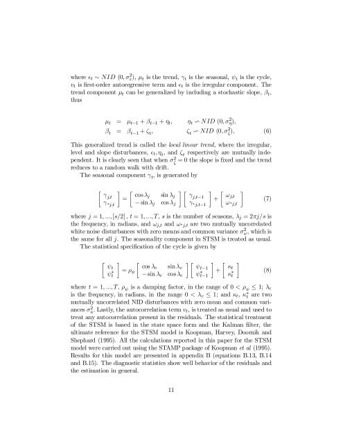
where ² t » NID (0; ¾ 2 "); ¹ t is the trend, ° t is the seasonal, Ã t is the cycle, v t is …rst-order autoregressive term and ² t is the irregular component. The trend component ¹ t can be generalized by including a stochastic slope, ¯t, thus ¹ t = ¹ t¡1 + ¯t¡1 + ´t; ´t v N ID (0; ¾ 2´); ¯t = ¯t¡1 + ³ t ; ³ t v NID (0; ¾ 2 ³ ); (6) This generalized trend is called the local linear trend, where the irregular, level and slope disturbances, ² t ; ´t; and ³ t respectively are mutually independent. It is clearly seen that when ¾ 2 ³ = 0 the slope is …xed and the trend reduces to a random walk with drift. The seasonal component ° t ; is generated by · °j;t ° ¤ j;t ¸ · cos = ¸j sin ¸j ¡ sin ¸j cos ¸j ¸ · °j;t¡1 °¤ j;t¡1 ¸ · !j;t + !¤ j;t ¸ (7) where j = 1; :::; [s=2] ; t = 1; :::; T; s is the number of seasons, ¸j = 2¼j=s is the frequency, in radians, and ! j;t and !¤ j;t are two mutually uncorrelated white noise disturbances with zero means and common variance ¾ 2 !; which is the same for all j. The seasonality component in STSM is treated as usual. The statistical speci…cation of the cycle is given by · Ãt Ã ¤ t ¸ · cos = ½ ¸c sin¸c Ã ¡sin ¸c cos ¸c ¸ · Ãt¡1 Ã ¤ t¡1 ¸ · + ·t ·¤t ¸ (8) where t = 1; :::; T; ½ Ã is a damping factor, in the range of 0 < ½ Ã · 1; ¸c is the frequency, in radians, in the range 0 < ¸c · 1; and ·t; ·¤t are two mutually uncorrelated NID disturbances with zero mean and common variances ¾ 2·: Lastly, the autocorrelation term v t, is treated as usual and used to treat any autocorrelation present in the residuals. The statistical treatment of the STSM is based in the state space form and the Kalman …lter, the ultimate reference for the STSM model is Koopman, Harvey, Doornik and Shephard (1995). All the calculations reported in this paper for the STSM model were carried out using the STAMP package of Koopman et al (1995). Results for this model are presented in appendix B (equations B.13, B.14 and B.15). The diagnostic statistics show well behavior of the residuals and the estimation in general. 11
3.6 Testing for Seasonal Unit Roots All the models above assumed di¤erent speci…cations regarding the stationarity of y t . For example, model (1) assumed that y t has non-seasonal unit roots and consequently a …rst-di¤erences …lter is used as the dependent variable. In model (2) the use of the seasonal …lter (twelve di¤erences) assumes that there are twelve unit roots in y t . Finally, model (3), which is a combination of (1) and (2), assumed the existence of thirteen unit roots in y t . As Franses (1996, 1999) argues, there are many cases where seasonal and/or …rst-di¤erences …lters are not relevant. Following this advise, we test for the presence of seasonal unit roots in y t using the approach proposed by Hylleberg et al. (1990). Under the null hypothesis, y t has twelve unit roots given the fact that the …lter (1 ¡ L 12 ) contains twelve unit roots which are 1; ¡1; §i; ¡0:5(1 § p 3i); 0:5(1 § p 3i); ¡0:5( p 3 § i); 0:5( p 3 § i), where the …rst root corresponds to the non-seasonal frequency (or frequency zero) and the other corresponds to di¤erent seasonal frequencies. Given that, the method for testing for seasonal unit roots consists of estimating (by OLS) the following regression Á(L)y 8t = ¹ t + ¼ 1 y 1t¡1 + ¼ 2 y 2t¡2 + ¼ 3 y 3t¡1 + ¼ 4 y 3t¡2 (9) +¼ 5 y 4t¡1 + ¼ 6 y 4t¡2 + ¼ 7 y 5t¡1 + ¼ 8 y 5t¡2 +¼ 9 y 6t¡1 + ¼ 10 y 6t¡2 + ¼ 11 y 7t¡1 + ¼ 12 y 7t¡2 + ² t where y 1t = (1 + L)(1 + L 2 )(1 + L 4 + L 8 )y t , y 2t = ¡(1 ¡ L)(1 ¡ L 2 )(1 + L 4 + L 8 )y t , y 3t = ¡(1 ¡ L 2 )(1 + L 4 + L 8 )y t , y 4t = ¡(1 ¡ L 4 )(1 ¡ p 3L + L 2 )(1 + L 2 + L 4 )y t , y 5t = ¡(1 ¡ L 4 )(1 + p 3L + L 2 )(1 + L 2 + L 4 )y t , y 6t = ¡(1¡L 4 )(1¡L 2 +L 4 )(1¡L+L 2 )y t , y 7t = ¡(1¡L 4 )(1¡L 2 +L 4 )(1+L+L 2 )y t , and y 8t = (1 ¡ L 12 )y t . The critical values for the t b¼1 , t b¼2 , F b¼3 ;b¼ 4 , F b¼5 ;b¼ 6 , F b¼7 ;b¼ 8 , F b¼9 ;b¼ 10 , and F b¼11 ;b¼ 12 have been tabulated by Hylleberg et al. (1990). Equation (9) was estimated for the three time series using a maximum lag of 36 to obtain non-autocorrelated residuals. Unit root test results are presented in Table 2 in the appendix A. Given the results, we apply the corresponding …lters to each time series to construct a new dependent variable. Speci…cation tests for estimating an ARMA(p; q) model using these “…ltered” series is given in appendix B. Diagnostic checks show well …t (except for ARCH in tranborder and domestic series). 4 Evaluating Forecasts In general, the fact that a model ‘best’ …ts the data does not necessarily mean that this model also renders better out-of-sample forecasts. This is the case 12
Page 1 and 2: DÉPARTEMENT DE SCIENCE ÉCONOMIQUE
Page 3 and 4: Abstract This paper uses six time s
Page 5 and 6: 2 Canadian Air Passenger Data In th
Page 7 and 8: 0.1 Jan 0.2 0.1 Feb 0.1 March 0.0 0
Page 9 and 10: meaningful elasticities for each ai
Page 11 and 12: dummy variables. Dummy variables ar
Page 13: where the disturbance ² t is assum
Page 17 and 18: The …rst forecast evaluation crit
Page 19 and 20: as di¤erent ‘scenario’ forecas
Page 21 and 22: [6] Dickey, D.A. and W.A. Fuller (1
Page 23 and 24: 6 Appendix A In this appendix we pr
Page 25 and 26: Table A.3. Canadian Air Passenger M
Page 27 and 28: Table A.5. Forecast comparisons and
Page 29 and 30: 7 Appendix B In this appendix, we p
Page 31 and 32: Equation B.3. Estimated AR Model fo
Page 33 and 34: Equation B.6. Estimated SUR Model f
Page 35 and 36: Equation .B.10. Estimated PAR Model
Page 37 and 38: Equation B.12. Estimated PAR Model
Page 39 and 40: Equation B.14. Estimated Filtered A
Page 41 and 42: Equation B.17. Estimated STSM Model
Page 43 and 44: 8 Appendix C In this appendix, the
Page 45 and 46: Equation C.3. Estimated AR Model fo
Page 47 and 48: Equation C.5. Estimated AR Model fo
Page 49: Equation C.7. Estimated STSM Model

0306E - Faculty of Social Sciences - UniversitÃ© d'Ottawa

Create successful ePaper yourself

Delete template?

Save as template?